Attracting fixed points for heavy particles in the vicinity of a vortex pair

Abstract

We study the behaviour of heavy inertial particles in the flow field of two like-signed vortices. In a frame co-rotating with the two vortices, we find that stable fixed points exist for these heavy inertial particles; these stable frame-fixed points exist only for particle Stokes number $St<St_{cr}$. We estimate $St_{cr}$ and compare this with direct numerical simulations, and find that the addition of viscosity increases the $St_{cr}$ slightly. We also find that the fixed points become more stable with increasing $St$ until they abruptly disappear at $St=St_{cr}$. These frame-fixed points are between fixed points and limit cycles in character.

I Introduction

Vortices are building blocks of turbulent fluid flow. During their evolution, vortices stretch, rotate and interact with other vortices. Energy in turbulent flows is transferred to larger and smaller scales by vortex mergers and stretching respectively. In the Earth’s atmosphere, in industrial processes and in water bodies, turbulent flows often carry particles such as dust or aerosols with them. Such particles are typically heavier than the fluid which carries them, and this paper is devoted to the effect of vortices on heavy particles. A large number of simulations and experiments Davilla and Hunt (2001); Benczik et al. (2002); Bec (2003); Chen et al. (2006); Derevyanko et al. (2007); Goto and Vassilicos (2008); Tallapragada and Ross (2008); Toschi and Bodenschatz (2009); Eidelman et al. (2010); Perlekar et al. (2011); Gibert et al. (2012) have shown that the transport of inertial particles in two- and three-dimensional turbulence is not like the transport of inertialess particles. In particular, inertial particles cluster. The primary reason for this in a turbulent flow is vorticity, and the tendency of heavy inertial particles to leave the neighborhood of a vortex. What happens when there is more than one vortex? Could heavy particles in fact have long residence times near vortices?

We choose the simplest flow with more than one vortex, namely the flow generated by two identical vortices of the same sign at a distance $2R$ from each other. Kinematics dictates that these vortices, when there is no viscosity, will cause each other to rotate around the origin at an angular velocity $\Omega$. This flow, for particles of a given small Stokes number, is shown below to display ‘fixed’ points in a moving frame of reference. An important consequence of this is that particles cluster in a location of low vorticity, but close to the vortices. These cluster points rotate with the flow. The location of cluster is different for different Stokes number, and vanishes beyond a critical Stokes number. The behavior is first analyzed in an inviscid framework, and followed by viscous simulations to show that the same behavior is displayed there as well.

The rest of the paper is organized as follows. We first describe our system and approach, and then present an analytical investigation of heavy particles in the like-signed vortex-pair flow. This is followed by a presentation of our point vortex simulations and a linear analysis. We end with a discussion of our direct numerical simulations, and conclusions.

II Elliptic Fixed Points in Lab and Rotating Frames of Reference

We begin by describing the system and the equations we use for heavy particles – first in the lab-frame and then in a frame rotating with the vortices – and then discuss why elliptic fixed points in a lab-fixed frame of reference are very different from those in a rotating frame of reference. Heavy particles cannot cluster in the vicinity of the former as proved in Ref.Sapsis and Haller (2010) but we show that they can and do cluster in the vicinity of the latter.

In the lab frame, we have two like-signed point vortices, each of circulation $\Gamma$ and placed at a distance of $2R$ from the other, describing motion on a circle of radius $R$, with a time period $T=8\pi^{2}R^{2}/\Gamma$. The vortices remain in antiphase from each other. The fluid velocity at a point $\mathbf{r}$ is given by:

$$\mathbf{u}_{\mbox{lab}} = \frac{d\mathbf{r}}{dt}=\frac{\Gamma}{2\pi}\mathbf{e}_{z}\times\left(\frac{\mathbf{r}-\mathbf{R}}{\left|\mathbf{r}-\mathbf{R}\right|^{2}}+\frac{\mathbf{r}+\mathbf{R}}{\left|\mathbf{r}+\mathbf{R}\right|^{2}}\right)\mbox{,}$$ (1)

where the vortices are at $\pm\mathbf{R=}\left(\pm X,\pm Y\right)$, and $\mathbf{e}_{z}$ is the unit vector pointing out of the page. The subscript ‘lab’ denotes that something is measured in the lab-fixed frame of reference.

The motion of rigid, inertial point particles is modeled by using the Maxey-Riley equations Maxey and Riley (1983) in the lab frame:

$$\frac{d\mathbf{\mathbf{x}}}{dt} = \mathbf{\mathbf{v}}$$

$$\frac{d\mathbf{\mathbf{v}}}{dt} = -\frac{1}{St}(\mathbf{v}-\mathbf{u})+\beta\frac{D\mathbf{u}}{Dt}$$ (2)

where $\beta=3\rho_{f}/(2\rho_{p}+\rho_{f})$, $\rho_{p}$ and $\rho_{f}$ are the particle and fluid densities respectively, $\mathbf{v}$ and $\mathbf{u}$ are the particle and fluid velocities respectively, and $\mathbf{x}$ the location of a particle, $St=\tau/T$ is the Stokes number, $\tau=\frac{2}{9}\frac{a^{2}}{\nu}\frac{\rho_{p}}{\rho_{f}}$ is the relaxation time of the particle, and $T$ is a characteristic time scale of the flow, taken here to be the time period of rotation. Light particles ($\rho_{p}\ll\rho_{f}$ i.e., $\beta\approx 3$) cluster in the regions of vortices whereas, heavy particles, such as aerosols, $\rho_{p}\gg\rho_{f}$ ($\beta=0$) are expelled from vortical regions Sapsis and Haller (2010).

In the frame of reference rotating with the same angular velocity as the vortices [$\Omega=\Gamma/(4\pi R^{2})$], the flow field is divided into water-tight compartments by the separatices – invariant manifolds, see e.g. Rom-Kedar et al. (1990); Newton (2001) – shown in figure 1. The equations of motion (2) may be transformed to this rotating frame and are given below. Quantities with a $\hat{}$ are measured in the rotating frame.

$$\frac{d\hat{\mathbf{x}}}{d\hat{t}} =\hat{\mathbf{v}}$$

$$\frac{d\hat{\mathbf{v}}}{d\hat{t}} =\frac{\hat{\mathbf{u}}-\hat{\mathbf{v}}}{St}-2\bm{\Omega}\times\mathbf{\hat{v}}+\Omega^{2}\mathbf{\hat{r}}$$ (3)

For $St=0$, the system has two fixed points (centers) at $(0,\pm\sqrt{3}R)$ in the rotating frame of reference. The elliptic nature of these fixed points may be seen by linearizing the velocity field at these points [see section (III.1)]. These ‘fixed-points’ are actually rotating at the same angular velocity as the vortices in the lab-fixed frame, so what we have are moving fixed points!

Incidentally we would like to distinguish our rotating frame of reference from the one that is normally used to simulate, for instance, Earth’s rotation. In the latter, the rotation of the lab is imposed as an additional forcing. Our lab is not rotating, but our flow is steady in a non-inertial frame that rotates with the angular velocity of the vortex pair. We also note that the points at $(0,\pm\sqrt{3}R)$ are fixed points for fluid particles and tracer particles, and not necessarily for inertial particles.

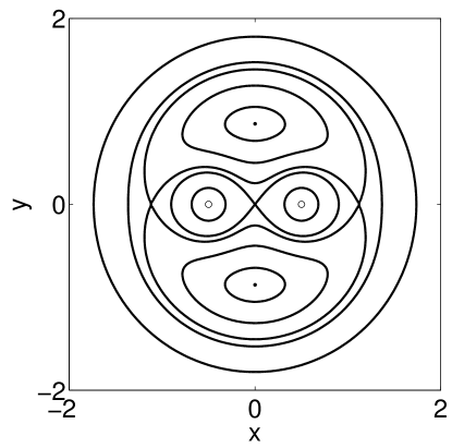
Figure 1: Invariant manifolds in the rotating frame in the flow around two identical point vortices. The vortices are indicated by the small circles at $\left(\pm 0.5,0\right)$, and the elliptic fixed points of our interest by the filled circles at $\left(0,\pm\sqrt{3}/2\right)$.

As previously mentioned, elliptic fixed points in the rotating frame of reference are qualitatively different from elliptic fixed points in a lab fixed frame of reference. Sapsis & Haller Sapsis and Haller (2010) show that the fixed points in a region of the flow consisting of elliptic streamlines cannot be attractors for heavy particles of small Stokes number. Their argument is that since $\beta\simeq 0$ for heavy particles, at $O\left(St\right)$ $\mathbf{u}$ may be used to replace $\mathbf{v}$ on the left hand side of eq. (2), to get

$$\mathbf{v}=\mathbf{u}-St\frac{D\mathbf{u}}{Dt}+\mathcal{O}\left(St^{2}\right),$$ (4)

where $\frac{d\mathbf{v}}{dt}$ was replaced with $\frac{D\mathbf{u}}{Dt}$ in the second term. This is called the ‘inertial equation’. The divergence of $\mathbf{v}$, since $\mathbf{u}$ is divergence-free in incompressible flow, becomes

$$\nabla\cdot\mathbf{v}=-St\nabla\cdot\left(\mathbf{u}\cdot\nabla\mathbf{u}\right)=-St\frac{\partial u_{i}}{\partial x_{j}}\frac{\partial u_{j}}{\partial x_{i}}=StQ\mbox{,}$$ (5)

where $Q=\left(\omega^{2}-s^{2}\right)$ is the Okubo-Weiss parameter, $s$ and $\omega$ being the symmetric and anti-symmetric parts of the strain-rate tensor respectively. A word of caution: in a general turbulent flow we must remember that particle velocities do not form a field, in the sense that there can be two very different particle velocities at the same location, so strictly speaking we may not define a quantity called divergence for particle velocity. However, at small Stokes numbers, the inertial equation allows $\mathbf{v}$ to be approximated to a field, and thus lets us relate this quantity to particle clustering for negative divergence and to particles leaving the neighborhood at positive divergence. At an elliptic fixed point in a lab-fixed frame, we must have $Q>0$, and Liouville’s theorem may be applied to a small volume in its vicinity to show that it cannot attract heavy particles. There is thus no attracting elliptic fixed point for small Stokes number heavy particles in a fixed frame of reference.

How about in a rotating frame of reference? We saw in the flow under consideration that there are two elliptic fixed points for tracer particles in the rotating frame. We next ask whether there are fixed points for inertial particles as well, i.e., are there locations where an inertial particle would remain forever. This may be done by solving for fixed points of eq. 3, giving

$$\frac{\hat{\mathbf{u}}}{St}=-\Omega^{2}\mathbf{r}.$$ (6)

Equation (6) has to be solved numerically. This was done using the MATLAB function minimisation routine “fsolve”. Solutions for eq. 6 exist for $St<St_{cr}=0.04264543$. For $St>St_{cr}$, the minima of $\hat{\mathbf{u}}+St\Omega^{2}\hat{\mathbf{r}}$ are greater than zero; i.e., there exist no solutions. Solutions of eq. 6 lying in the top half-plane is shown in figure 2. A symmetrically placed fixed point exists with $x<0,y<0$. We see that the fixed points start on the y-axis at $\sqrt{3}R$ for particles of $St=0$, and move progressively away from the vertical as $St$ increases. Thus particles of increasing inertia display fixed points which drift further and further away from the axis of symmetry. One may imagine that with inertia, the particles find it harder to “keep up” with the rotating frame and drift in the opposite direction. Note that the fixed points lie within the region of the flow where the streamlines form closed orbits. We therefore refer to them as particle fixed points in the elliptic region. We also alternatively refer to them as the finite $\mathbf{r}$ fixed points. Now that we have the exact solution for the fixed points, we may assess how good the $\mathcal{O}\left(St\right)$ approximation is, by substituting $\mathbf{v}$ from eq. (4) into (6). We obtain fixed points, also shown in figure 2, that are accurate to $\mathcal{O}\left(St\right)$, as expected.

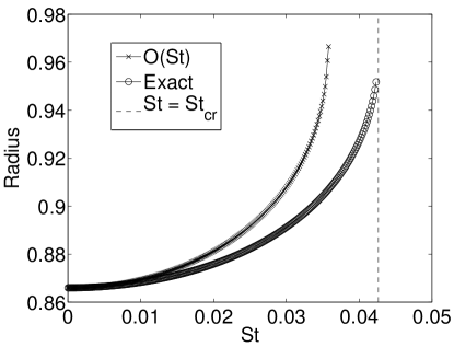
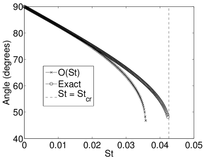
Figure 2: Locations of fixed points (in radians) for inertial particles with different Stokes number obtained from eq. (6) (circles). We also show the location of fixed points obtained by using the small Stokes number ($\mathcal{O}(St)$) approximation (cross). There are no fixed points for $St>St_{cr}$. [Here and in all figures to follow, simulations were done with $\Gamma=2\pi$. ]

III Point vortex simulations

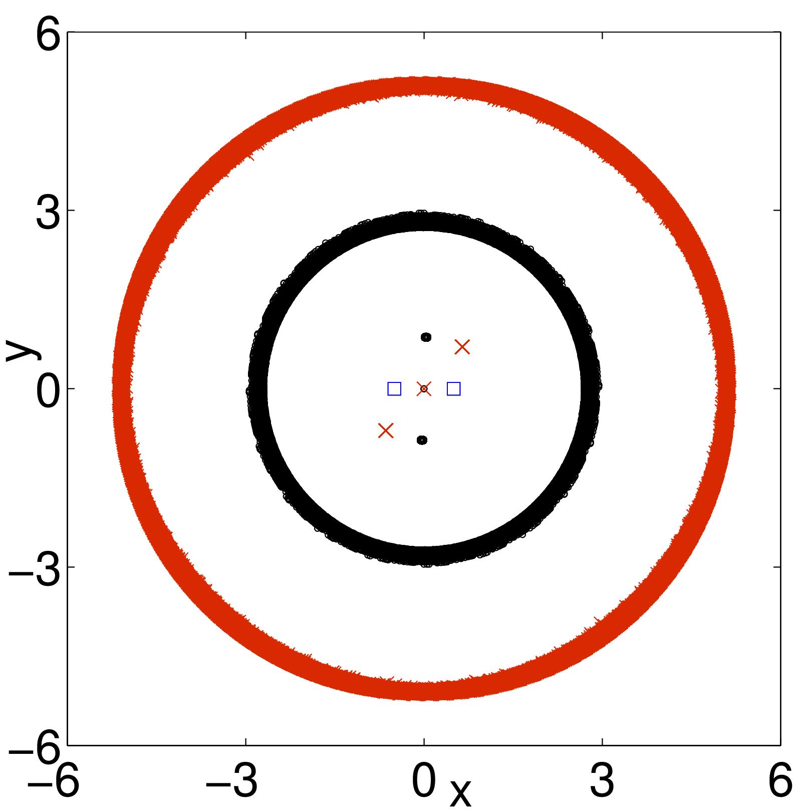
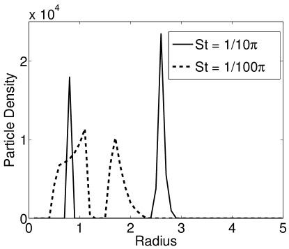
Figure 3: (Left) Particle locations after $100T$ for $St=1/100\pi$ (black) and $1/7.5\pi$ (red). The fixed points are the filled circle and the crosses respectively. The phase chosen is when the point vortices, indicated by blue squares, lie on the horizontal axis. (In the figure, the thickness of outer ring-clusters is exaggerated.) (Right) Particle density versus radius after 10 time periods. The density profiles narrow with time. At a higher Stokes number, the particles are more sharply clustered. Also as Stokes increases, the nonlinear wave propagates outwards faster, so the second peak is seen at a bigger radius.

We perform inviscid numerical simulations for a range of Stokes numbers. We start with $5\times 10^{4}$ particles uniformly distributed over a region encompassing the invariant manifolds. We use $\Gamma=2\pi$ unless otherwise mentioned. Figure 3 shows the particle locations after $100$ time periods of rotation, for two Stokes numbers. In each case there are three fixed points at which heavy particles cluster: the fixed point at $|\mathbf{r}|=\infty$ (which exists because any nonzero inertia in a heavy particle centrifuges the particle out from a region of rotating motion), as well as the symmetric pair we have discussed. This pair, lying within the elliptic flow region, is indicated in the figure, and although not apparent, a very large number of particles are clustered at these. The new fixed points for inertial particles are thus attracting fixed points. The other fixed point, $|\mathbf{r}|=\infty$, attracts all particles which begin at a large distance away from the origin, since for them the system may effectively be replaced by a single vortex of twice the circulation, i.e., $2\Gamma$. The evolution of these particles would take the form of a nonlinear wave Raju and Meiburg (1997), with a clumping that depends on Stokes number. In addition, the $|\mathbf{r}|=\infty$ fixed point has a basin of attraction within our region of interest. Particles which will travel towards $|\mathbf{r}|=\infty$ are seen as a circle of clustered points in figure 3(left). The radius of this cluster is a slowly increasing function of time, going as $r\sim t^{1/4}St$ at large $r$. This is because, at large $r$, the two vortices act predominantly act as one larger vortex of twice the strength and the equation of motion in radial coordinates for particles around a single vortex is $dr/dt\sim St/r^{3}$ (see, e.g., Raju and Meiburg (1997)). That particles form dense clusters at the fixed points is seen in the radial density profile of figure 3(right), at a particular instant of time. Two regions of clumping are evident. The inner one corresponding to the elliptic-region fixed points remains there, but the outer spike slowly moves towards $|\mathbf{r}|=\infty$. With time, the clumps become narrower and taller. With increasing inertia too, the clumps become sharper, but not necessarily taller. At higher inertia, the profile increasingly resembles a double spike. The total number of particles clustered at the inner fixed points decreases with inertia, as we shall discuss soon, and at some Stokes number we no longer have any fixed points at finite $r$.

Applying the inertial equation (eq.4) to this problem, rather than the complete force balance, has the effect of omitting the second time derivative of the radial location of a particle, and for a single vortex Raju & Meiburg Raju and Meiburg (1997) show that this approximation becomes exact at long times.

Basin boundaries of each fixed point are shown in figure 4. Particles which begin their lives inside the regions shown in red are attracted to one of the fixed points at finite radius and particles in the other regions drift away to infinity. As the Stokes number increases, the basin of attraction of the finite $r$ fixed points shrinks in size. These basins of attraction disappear completely for $St>St_{cr}$, along with the fixed points themselves. At very low inertia, the spirals are very tightly wound. It may be argued from the radial velocity of an inertial particle moving around a single vortex that the spacing between two crossings must be proportional to $St$. Thus two particles which begin life very close to each other, but in the basin boundaries of different attractors, have vastly different fortunes. One gets trapped forever in the vicinity of the vortices while the other is slowly centrifuged out to infinity.

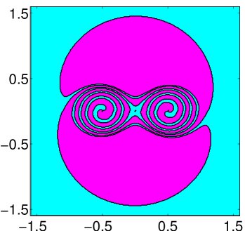
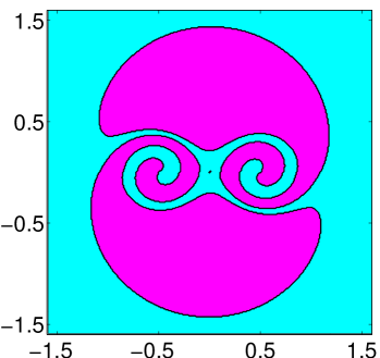
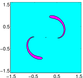
Figure 4: Basins of attraction of the fixed points for $St=1/300\pi$ (top left), $1/100\pi$ (top right), $1/20\pi$ (bottom left), and $1/7.5\pi$ (bottom right). The red region shows the basin of attraction of one of the finite $\mathbf{r}$ fixed points. Particles in the blue region escape to infinity.

In figure 5, we plot the number of particles starting from a uniform grid over a domain $\left(-1.6,1.6\right)\times\left(-1.6,1.6\right)$ that are attracted to one of the two fixed points. Because we started with uniformly distributed points, this is proportional to the area of its basin of attraction. It is seen that close to the critical Stokes number, the rate of decrease of the number of particles is very high, the graph being practically vertical, indicative of a finite-Stokes singularity. The reason for this singular behavior is not clear to us at this point.

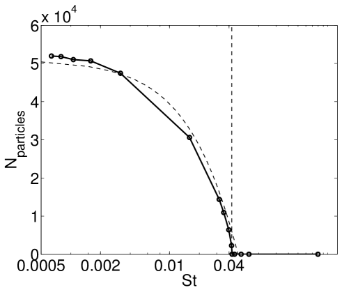
Figure 5: The number of particles in each simulation that are attracted to the finite $\mathbf{r}$ fixed points. This number is proportional to the area of the basin of attraction. A quadratic fit is provided just to guide the eye. The vertical line indicates $St=St_{cr}$.

III.1 Linear analysis near the particle fixed points

Behavior in the vicinity of the inertial particle fixed points is obtained by linearising the particle dynamics in the rotating frame (eq. (3)) along the lines of Bec (2005). At the fixed point, we have $\hat{\mathbf{v}}_{fp}=0$ and $\hat{\mathbf{u}}_{fp}=-St\mbox{$\left(\Omega^{2}\hat{\mathbf{r}}\right)$}$. This gives, for the linear perturbations,

$$\frac{d\left(\delta\hat{\mathbf{x}}\right)}{d\hat{t}} =\delta\hat{\mathbf{v}}$$

$$\frac{d\left(\delta\hat{\mathbf{v}}\right)}{d\hat{t}} =\frac{\delta\hat{\mathbf{u}}-\delta\hat{\mathbf{v}}}{St}-2\bm{\Omega}\times\left(\delta\mathbf{\hat{v}}\right)+\Omega^{2}\delta\mathbf{\hat{r}}$$ (7)

The derivatives on the LHS of eq. (7) are derivatives along particle trajectories. The perturbation fluid velocities in the RHS are calculated by differentiating the Biot-Savart law. The eigenvalues of the linearised velocity equations are plotted in figure (6). One of the eigenvalues crosses zero at the crititcal Stokes number. It is also worth noting that the slopes of the eigenvalue curves diverge at $St=St_{cr}.$

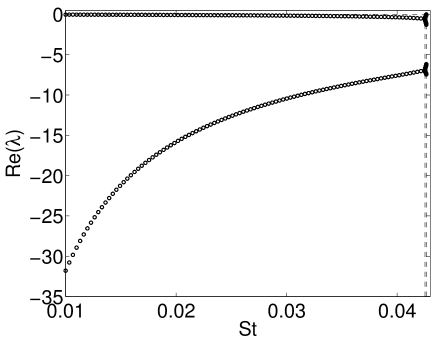
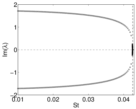
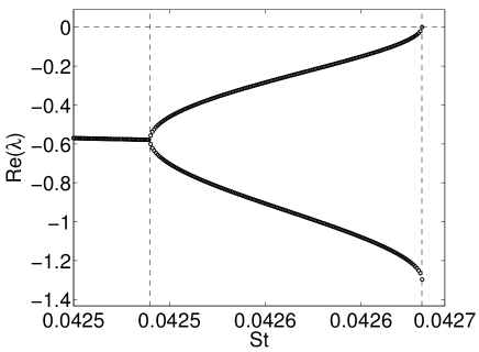
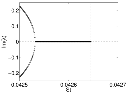
Figure 6: Real and imaginary parts of the eigenvalues of eq. 7. The two vertical dashed lines are at values of $St$ where a) the two pairs complex conjugate eigenvalues become wholly real, and b) at $St=St_{cr}$. The values for these Stokes numbers may be found in the text. The figures at the bottom are zoomed-in near $St_{cr}$. The real part crosses zero (at an infinite slope) at $St_{cr}$.

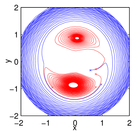
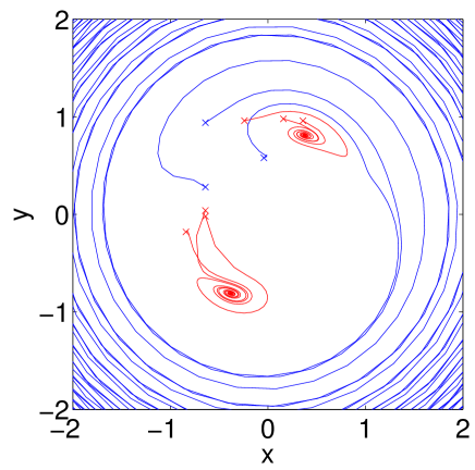
Figure 7: Particle trajectories for representative Stokes numbers of $St=1/50\pi$ (left) and $St=1/10\pi$ (right) showing that the fixed points in the rotating frame are spiral nodes. The crosses indicate starting positions for the particles. Trajectories in blue leave the vicinity of the vortices and centrifuge out to infinity. Trajectories in red fall into one of the fixed points.

At $\mathcal{O}\left(St\right)$, a negative Okubo-Weiss parameter is a necessary condition for the existence of an attracting fixed point. We have seen from the argument of Sapsis & Haller Sapsis and Haller (2010) that this cannot happen in a neighborhood of closed streamlines in a fixed frame of reference. Things are different in a rotating frame: we may have a negative divergence of particle velocity in a neighborhood of streamlines that are closed paths in the rotating frame. The velocity in the rotating frame is (quantities with $\hat{}$s are measured in the rotating frame)

$$\hat{\mathbf{v}}=\hat{\mathbf{u}}-\tau\left(\frac{d\hat{\mathbf{u}}}{d\hat{t}}+2\vec{\Omega}\times\hat{\mathbf{u}}-\Omega^{2}\hat{\mathbf{r}}\right)\mbox{,}$$

giving, for the divergence of the particle velocity,

$$\hat{\nabla}\cdot\hat{\mathbf{v}}=-\tau\left(\frac{\partial\hat{u}_{i}}{\partial\hat{x}_{j}}\frac{\partial\hat{u}_{j}}{\partial\hat{x}_{i}}+2\hat{\nabla}\cdot\left(\bm{\Omega}\times\hat{\mathbf{u}}\right)-2\Omega^{2}\right)=-\tau\left(\frac{\partial\hat{u}_{i}}{\partial\hat{x}_{j}}\frac{\partial\hat{u}_{j}}{\partial\hat{x}_{i}}-2\bm{\Omega}\cdot\hat{\bm{\omega}}-2\Omega^{2}\right)$$

$$\hat{\nabla}\cdot\hat{\mathbf{v}}=-\tau\left(\frac{\partial\hat{u}_{i}}{\partial\hat{x}_{j}}\frac{\partial\hat{u}_{j}}{\partial\hat{x}_{i}}+2\Omega^{2}\right)\mbox{, }$$

where $\hat{\bm{\omega}}=-2\Omega\mathbf{e}_{z}$ is the vorticity in the rotating frame and the summation convection has been used. The first product on the right hand side may be shown to be equal to $S_{ij}S_{ij}-2\Omega^{2}$, making the divergence of particle velocity equal to

$$\nabla\cdot\mathbf{\hat{v}}=St{\hat{Q}},$$ (8)

where $\hat{Q}$ is the Okubo-Weiss parameter in the rotating frame.

The quantity $(S_{ij}S_{ij})$ is plotted in figure 8, and seen to be positive in the vicinity of the attracting fixed point, making the Okubo-Weiss parameter negative; we thus satisfy the necessary condition for the existence of attracting fixed points, in a neighborhood where fluid particles follow elliptical streamlines.

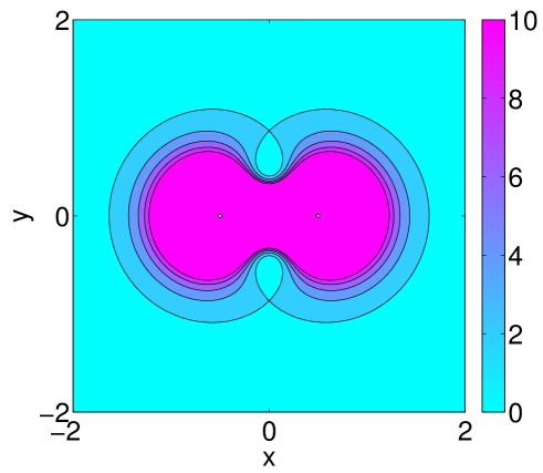
Figure 8: Contour-plot of $S_{ij}S_{ij}$. The negative of this quantity, $\hat{Q}$, is the Okubo-Weiss parameter, which is proportional to the divergence of particle velocity.

IV Navier-Stokes Simulations

We now substantiate our results by studying the above flow in a more realistic setting: by including viscosity and beginning with Lamb-Oseen vortices, in contrast to the point vortices of section III. The flow obeys the two-dimensional Navier-Stokes equations

$$D_{t}\omega=\nu\nabla^{2}\omega\mbox{ , }-\nabla^{2}\psi=\omega,$$ (9)

where $\omega$ is the vorticity, $\nu$ is the kinematic viscosity, $\psi$ is the streamfunction, i.e. ${\bf u}=(-\partial_{y}\psi,\partial_{x}\psi)$, and $D_{t}\equiv\partial_{t}+{\bf u}\cdot\nabla$ is the material derivative. Particles obey eq. (2). We use a square domain with each side of length $L=2\pi$ and employ periodic boundary conditions. Eqs.(9), and the continuity equation are numerically integrated using a pseudo-spectral method. Time-advancement is done using an exponential Adams-Bashforth scheme. Space is discretized with $N^{2}$ collocation grid points. We have verified (not shown here) that grid-convergence is achieved by conducting simulations with varying grid resolutions $N=128$ and $N=256$ and obtaining the same results. In what follows, we have used $N=256$ unless stated otherwise.

We initialize the simulation with two Gaussian vortices positioned at $(x_{1},y_{1})$ and $(x_{2},y_{2})$, of vorticity

$$\omega_{1}(x,y) = \omega_{0}\exp[-(r_{1}/r_{0})^{2}]\ {\rm{and}}$$ (10)

$$\omega_{2}(x,y) = \omega_{0}\exp[-(r_{2}/r_{0})^{2}].$$ (11)

Here, $r_{0}$ is the width of the vortex, $\omega_{0}$ denotes the vortex amplitude, $r_{1}^{2}=(x-x_{1})^{2}+(y-y_{1})^{2}$ and $r_{2}^{2}=(x-x_{2})^{2}+(y-y_{2})^{2}$ and the separation between the centers of the vortices $\ell\equiv(y_{2}-y_{1})^{2}+(x_{2}-x_{1})^{2}$ is kept fixed at $\ell=0.9818$ (we obtain this value because we choose an integer number of grid-spacings). We fix $r_{0}=\pi/32$, $\omega_{0}=2^{11}/\pi\approx 652$ (these values are tuned so that the timeperiod of rotation is $T\approx 1$), $\nu=10^{-4}$ giving $Re=10^{4}$, and vary $St$ from $0$ to $0.05$. We start the simulation with $N_{p}=10^{3}$ particles distributed randomly over the entire domain and study how particle distribution evolves.

An identical same-signed vortex pair will ultimately merge, In the first stage of this process, the vortices go around each other in a fashion very similar to the inviscid case. During this phase, they also diffuse out slowly. When the radius of the vortices reaches a quarter of the separation between them, a second stage in the merger process begins, with a significant and sudden increase in the radial component of the velocity of the vortices, drawing them towards each other. The Reynolds number in this simulation is $Re=10^{4}$, which means, given the initial radius, that the vortices complete about 90 complete cycles, up to a time of $t=86$ before the second stage of the merger process begins. We note that particles with $St\sim\mathcal{O}\left(1/T\right)$, (where $T=86$ timeperiods) would have fallen into the fixed points before the merger process begins. The cluster at the fixed point thus has a long life before the merger process is completed, after which it begins a slow drift away from the merged vortex. We are interested here in what happens to the cluster during the first phase of the merger process. Figure 9 shows a snapshot of the particle positions and contours of the vorticity at $t=10$ for $St=0.027$. The cluster at the fixed point is remarkably similar to the one seen in the inviscid case, as is evident when one compares this figure with fig. 3. Figure 10 shows the radial distance at which particles cluster (measured from the point halfway between the vortex centres) as a function of time, showing that, for this Stokes number$=0.03$, (which is below $St_{cr},$) the cluster at the fixed points is remarkably stable for a long time. Figure 11 compares the fixed points obtained from the viscous and inviscid simulations. The critical Stokes number is slightly higher in viscous simulations.

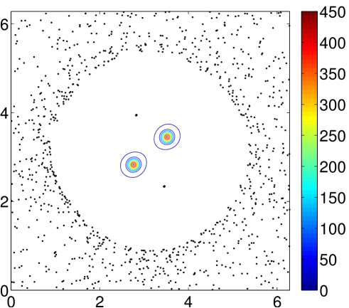
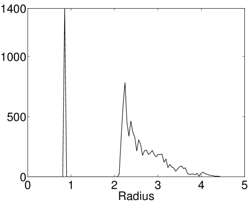
Figure 9: LEFT: Plot of particle positions and vorticity contours at $t=10$ for $St=0.027$. The fixed point can be seen at ($\pi\pm 0.32$,$\pi\pm 0.8)$.
RIGHT: Plot of particle density showing versus radius.

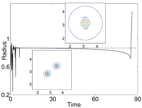
Figure 10: The radial location of the fixed point time for a viscous simulation. Inset in the figure are the contours of vorticity at $t=10$ and $t=86$ for $St=0.03$. The maxima of vorticity are at $\omega=452$ and $\omega=132$ respectively. The dashed line is $r=\sqrt{3}/2$ . Since we are interested to look at times equal to and larger than merger time, we use $N^{2}=1024^{2}$ collocation points.

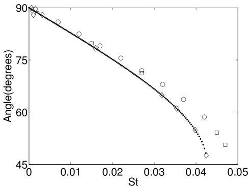
Figure 11: Fixed point predictions (at $t=50$). We plot the angle the line joining the fixed points makes with the line joining the centres of the vortices. The dots are exact solutions. The diamonds are point-vortex solutions. The circles and squares are DNS results for grid resolutions of $256^{2}$ and $512^{2}$ respectively.

V Conclusion

We have shown that apart from fixed points in the lab frame, clustering can be governed by fixed points in a rotating frame. Fixed points for heavy particles of small Stokes number do not coincide with those for tracer particles, but lie in the vicinity. The location of these fixed points is within a region where fluid particles follow elliptical trajectories. Contrary to our understanding of elliptic fixed points in the lab-fixed frame, these fixed points in a rotating frame can be attractive, which is the reason for clustering. Note that these moving fixed points are not limit cycles, because the phase is fixed.

The study here is on a simple model flow, but has relevance to particle dynamics in turbulence. Persistence times for particles near vortices are important in turbulent flows. With attracting fixed points in the vicinity of point vortices, the persistence times are in principle infinite. In cloud dynamics, for instance, we believe these fixed points in rotating frames could contribute to droplet clustering and therefore change the droplet size distributions. Our study indicates that regions of particle clustering may have to be calculated for frames of reference that are themselves not fixed. These frame-fixed points may be expected to have the same effect on the carrier flow as fixed points in the lab frame.