Fermi liquid theory of resonant spin pumping

Abstract

We study resonant all-electric adiabatic spin pumping through a quantum dot with two nearby levels by using a Fermi liquid approach in the strongly interacting regime, combined with a projective numerical renormalization group (NRG) theory. Due to spin-orbit coupling, a strong spin pumping resonance emerges at every charging transition, which allows for the transfer of a spin $\sim\hbar/2$ through the device in a single pumping cycle. Depending on the precise geometry of the device, controlled pure spin pumping is also possible.

Introduction: Spin-orbit (SO) coupling plays a prominent role in many different fields of physics: it is not only responsible for magnetic anisotropy and thus determines the orientation and low energy excitation spectra of magnets and magnetic molecules Žutić et al. (2004), but its presence also changes the universality class of the localization transition Lee and Ramakrishnan (1985), and it is also a crucial component for realizing topological insulators Brüne et al. (2011); Kells et al. (2012); Brouwer et al. (2011). The SO coupling plays also a determining role in mesoscopic physics, in spintronics, and, most importantly, in spin-based quantum computation. In the latter context, in particular, it produces spin relaxation in spin quantum bits Khaetskii and Nazarov (2000); Burkard et al. (1999) and leads to geometrical spin relaxation even in the absence of external magnetic fields San-Jose et al. (2006), however, it can also be used to generate effective magnetic fields and achieve electrical spin control  Nowack et al. (2007).

It has been first observed in Ref. Brouwer (1998) that, in the presence of SO interaction, one can produce a spin current by simply cycling adiabatically the parameters of a chaotic cavity (pumping) without breaking the instantaneous time reversal symmetry, i.e., without applying an external magnetic field. Obviously, realizing such spin pumps would enable one to reach an important goal of spintronics, and build all electric spin sources. Indeed, guided by this observation, more controlled setups have been proposed to pump spin currents through quantum wires Governale et al. (2003) and quantum dots Brosco et al. (2010), however, the effects of interactions were ignored in all these studies. While this is justified to a certain extent for the case of a quantum wire Governale et al. (2003), it is certainly unjustified for a quantum dot Brosco et al. (2010), where – precisely in the regime of interest – interactions are necessarily strong Brosco et al. (2010). Studying pumping through strongly correlated systems is a notoriously hard problem Citro et al. (2003). For charge pumping through quantum dots, several expressions have been derived based upon an adiabatic expansion of the Keldysh Green’s functions Sela and Oreg (2006); Governale et al. (2003). The expressions obtained, however, contain terms, which correspond to local charge oscillations, not related to true pumping. An alternative, perturbative approach of pumping has been developed in Ref. Rojek et al. (2013), but this method is restricted to the regime of weak tunneling and high temperatures, and cannot be used to reach the most exciting low temperature regime.

Here we revisit the problem studied in Ref. Brosco et al. (2010) and investigate how the interplay of SO coupling and strong electronic interactions influences spin pumping through a quantum dot at very low temperatures, deep in the strongly correlated regime. Our method is very different in spirit from those of Refs. Governale et al. (2003); Sela and Oreg (2006); Rojek et al. (2013), and rather, it follows lines similar to Ref. Aono, 2003: we start out from the observation that at $T=0$ temperature our quantum dot (similar to many interacting systems of interest) realizes a local Fermi liquid state. In this state, quasiparticle scattering at the Fermi energy is elastic, and can be characterized by a single particle on shell S-matrix. For very small pumping frequencies and small temperatures, $\omega,T\to 0$, the current through the device is carried by quasiparticles at or very close to the Fermi surface, where – to leading order – multiparticle scattering processes can be neglected by simple Fermi liquid phase space arguments. Then for the dominant elastic processes, Brouwer’s pumping formula can be applied, and the leading contribution to the pumped current can be expressed just in terms of the single particle S-matrix, evaluated at the Fermi energy. This adiabatic Fermi liquid approach is justified as long as $\omega$ and $T$ are less than the Fermi liquid scale (i.e. the level width $\Gamma$ in the mixed valence region considered here).

Computing the latter is still an extremely demanding task: we do that here in the most interesting narrow level limit by using a projective approach, whereby we first project the Hamiltonian to the subspace of Kramers degenerate levels participating in the pumping cycle, and then perform numerical renormalization group (NRG) calculations for this projected Hamiltonian and reconstruct the S-matrix. The strong Coulomb repulsion has a dramatic effect: in the vicinity of every charging transition, a spin pumping resonance (or antiresonance) emerges. As a consequence of large interaction, these resonances are well separated in parameter space, and the total spin pumped through them can reach values of $\sim\hbar/2$ in pumping cycles sketched in Fig. 1. These findings must be contrasted with the hight temperature results of Rojek et al. (2013) and also our non-interacting results, Ref. Brosco et al. (2010), where positive and negative pumping regions were found to appear close together in parameter space.

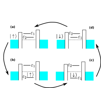
Figure 1: (Color online) Sketch of the spin pumping cycle. In the initial configuration one electron is injected into the dot. Due to the spin orbit interaction the spin up and spin down parts of the wave function are rotated differently (for clarity, only the spin up component is shown), and the spin up and spin down parts move into differnt electrodes, thereby resulting in spin pumping.

Model. We consider an interacting system with two almost degenerate levels, $\varepsilon_{1}$ and $\varepsilon_{2}$, close to the Fermi energy, and weakly coupled to external electrodes. The average energy $\bar{\varepsilon}=(\varepsilon_{1}+\varepsilon_{2})/2$ as well as the energy difference $\Delta\varepsilon=\varepsilon_{1}-\varepsilon_{2}$ of these levels can be tuned by applying several gate voltages to the same quantum dot (or chaotic cavity), as in the experiments of Ref. Miller et al., 2003. We shall thus consider these as pumping variables throughout this paper [$\bar{\varepsilon}=\bar{\varepsilon}(t)$ and $\Delta\varepsilon=\Delta\varepsilon(t)$]. By disregarding the other occupied or empty levels, we describe our system by the following Hamiltonian

$$H = \sum_{\sigma,j=\{1,2\}}\varepsilon_{j}(t)\,d^{\dagger}_{j\sigma}d_{j\sigma}+\sum_{\sigma}\bigl{(}t_{\sigma}d^{\dagger}_{1\sigma}\,d_{2\sigma}+h.c.\bigr{)}$$ (1)

$$+ \frac{U}{2}n(n-1)+\sum_{\sigma,j,r}v_{j}^{r}\left(d^{\dagger}_{j\sigma}\psi_{r\sigma}+h.c.\right)\,,$$

with $d^{\dagger}_{j\sigma}$ the creation operator of a spin $\sigma$ electron at level $j=1,2$, and $n$ the total number of electrons on the dot. For simplicity, we have chosen the spin quantization axis to coincide with the one dictated by the SO coupling, but otherwise assumed the most general single particle Hamiltonian allowed by time reversal symmetry. The parameters $t_{\sigma}=t+i\alpha\,\sigma$ describe spin dependent hybridization between the two levels with $\alpha$ the effective strength of the SO interaction. The term $\sim Un^{2}$ accounts for electron-electron interaction, while the last term of Eq. (1) describes the hybridization between the dot levels and the leads. The field $\psi^{\dagger}_{r\sigma}=\sum_{\mathbf{k}}c_{{\mathbf{k}},r\sigma}^{\dagger}/(\varrho_{r})^{1/2}$ creates a conduction electron in lead $r=L/R$ , and has been normalized by the density of states of the corresponding electrode, $\varrho_{r}$ so that the hopping amplitudes $v_{j}^{r}$ are dimensionless. We shall assume that the leads behave as regular Fermi liquids, and thus the dynamics of the creation operators $c_{{\mathbf{k}},r\sigma}^{\dagger}$ (and those of $\psi^{\dagger}_{r\sigma}$) are governed by free electron Hamiltonians.

The last term of Eq. (1) induces quantum fluctuations and a finite but asymmetrical broadening of the two levels. In the mixed valence regime discussed here, all energy scales must be compared to the strength of these quantum fluctuations, $\Gamma\equiv\sum_{i}\Gamma_{ii}\equiv 2\pi\sum_{r=L/R}\,{v^{r}_{i}}^{\ast}\,v^{r}_{i}$, which shall be used in what follows as an energy unit. The hybridization $v^{r}_{i}$ induces spin pumping as long as the two levels do not couple to the same linear combination of the leads, $\mathrm{det}(v^{r}_{i})\neq 0$ Brosco et al. (2010).

Formalism: As shown by Brouwer Brouwer (1998), for a noninteracting mesoscopic system, for adiabatical parameter changes, the accumulated charge and spin depend only on the path followed in parameter space, and can both be expressed in terms of the scattering matrix ${\cal S}_{rr}^{\sigma\sigma^{\prime}}$. Performing a cycle of area $A$ in the parameter space spanned by $\epsilon_{1}$ and $\epsilon_{2}$, e.g., one accumulates a spin

$$\Delta{\mathbf{S}}_{r}=\frac{\hbar}{2\pi}\int_{A}{\boldsymbol{\Pi}}^{(S)}_{r}(\epsilon_{1},\epsilon_{2})\,{\rm d}\epsilon_{1}{\rm d}\epsilon_{2}$$ (2)

in electrode $r$, where the spin pumping field is defined as

$${\boldsymbol{\Pi}}^{(S)}_{r}(\epsilon_{1},\epsilon_{2})={\rm Im\,Tr}\left\{\left(\Lambda_{r}\otimes{\boldsymbol{\sigma}}\right)\frac{\partial{\cal S}}{\partial\epsilon_{2}}\frac{\partial{\cal S}^{\dagger}}{\partial\epsilon_{1}}\right\}\;,$$ (3)

with $\Lambda_{r}$ a projector selecting scattering channels in electrode $r$. As explained in the introduction, here we shall exploit the fact that the ground state of Eq. (1) is a Fermi liquid Noziéres (1978). Therefore quasiparticles scatter elastically at $T\approx 0$, and their scattering can be described in terms of the single particle (on shell) S-matrix evaluated at the Fermi energy, $S_{rr}^{\sigma\sigma^{\prime}}(\omega=0)$. Since precisely these quasiparticles are responsible for adiabatic pumping, we can continue using (2) at very low temperatures, while replacing the noninteracting S-matrix in Eq. (3) by its many-body counterpart, ${{\cal S}}\to S(\omega=0)$. For our Hamiltonian, the latter can be simply related to the Fourier transform of the local Greens’s functions Borda et al. (2007), $G_{j\sigma,j^{\prime}\sigma^{\prime}}(t)\equiv-i\langle[d_{j\sigma}(t),d^{\dagger}_{j\sigma^{\prime}}(0)]\rangle\theta(t)$,

$$S_{rr^{\prime}}^{\sigma\sigma^{\prime}}(\omega)=\delta_{rr^{\prime}}\delta_{\sigma\sigma^{\prime}}-2\pi i\sum_{j,j^{\prime}}\,v^{r}_{j}\,{v^{r^{\prime}}_{j^{\prime}}}^{\ast}\,G_{j\sigma,j^{\prime}\sigma^{\prime}}(\omega).$$ (4)

Our task is thus reduced to compute $G_{j\sigma,j^{\prime}\sigma^{\prime}}(\omega)$ very precisely as a function of external parameters, and then compute the pumped spin. This, however, turns out to be a very challenging task since we need to determine with high precision both the imaginary and the real parts of $G_{j\sigma,j^{\prime}\sigma^{\prime}}(\omega)$ at the Fermi energy. Unfortunately, as of to date, none of the available methods can do that reliably.

Restricting ourself to the most interesting regime of a narrow resonance, $\sqrt{t^{2}+\alpha^{2}}\gg\Gamma$, however, we can considerably simplify the problem. For $U=0$ the isolated dot has two Kramer’s doublets at energies $E_{\pm}=\bar{\varepsilon}\pm\sqrt{t^{2}+\alpha^{2}+\Delta\varepsilon^{2}/4}$. Since $E_{+}-E_{-}\geq 2\sqrt{t^{2}+\alpha^{2}}\gg\Gamma$, for occupations, $\langle n\rangle\leq 2$ we can neglect the higher Kramers doublet, and project to the lower level, $E_{-}$. We thus introduce the operators

$$D^{\dagger}_{\sigma}\equiv\sum_{j}\Phi_{j,\sigma}d^{\dagger}_{j,\sigma}\,,$$ (5)

with the spinors $\Phi_{\sigma}$ parametrized most conveniently in terms of the angles $\varphi\equiv-\cot^{-1}(t/\alpha)$ and $\vartheta\equiv-\cot^{-1}(\Delta\epsilon/2\sqrt{t^{2}+\alpha^{2}})$ and expressed as $\Phi_{\uparrow}=\Phi_{\downarrow}^{\ast}=(\cos(\vartheta/2),e^{-i\varphi}\sin(\vartheta/2))$. The projected Hamiltonian is then just an ordinary Anderson Hamiltonian

$$H_{\rm proj} = \sum_{\sigma}E_{-}(\vartheta,\varphi)D^{\dagger}_{\sigma}D_{\sigma}+\frac{U}{2}n(n-1)$$

$$+ \tilde{v}(\vartheta,\varphi)\sum_{\sigma}\left(D^{\dagger}_{\sigma}\tilde{\psi}_{\sigma}+h.c.\right)\,,$$

with the hybridization defined as $\tilde{v}^{2}=\sum_{r}\bigl{|}{\tilde{v}}^{r}_{\uparrow}\bigr{|}^{2}$, with $\tilde{v}^{r}_{\uparrow}\equiv\sum_{j}\Phi_{j,\uparrow}^{\ast}v_{j,\uparrow}^{r}$. Within this approximation, the S-matrix of the original fields $\psi_{r,\sigma}$ can then be expressed as

$$S_{rr^{\prime}}^{\sigma\sigma^{\prime}}(\omega)=\delta_{\sigma\sigma^{\prime}}\,\bigl{\{}\delta_{r,r^{\prime}}-2\pi i\,\tilde{v}_{\sigma}^{r}\,{{\tilde{v}}_{\sigma}^{r^{\prime}\ast}}\,G_{D}(\omega)\bigr{\}},$$ (6)

with $G_{D}(\omega)$ the effective Anderson model’s local retarded propagator. At $T,\omega\to 0$ this S-matrix has two eigenvalues for both spin directions: a trivial eigenvalue, $s=1$, and an eigenvalue $s=e^{2i\delta}$, with the phase shift $\delta$ related to the occupation of the level $E_{-}$ by the Friedel sum rule, $\langle D_{\sigma}^{\dagger}D_{\sigma}\rangle=\delta/\pi$. The occupation $\langle D_{\sigma}^{\dagger}D_{\sigma}\rangle$ is a universal function of the ratios $\tilde{\Gamma}/U$ and $E_{-}/U$, with $\tilde{\Gamma}=2\pi\tilde{v}^{2}$ denoting the width of the level $E_{-}$, and can be determined reliably by functional or numerical renormalization group methods as well as by Bethe Ansatz. Together with Eq. (3), Eq. (6) thus provides a complete and simple description of adiabatic spin pumping through the device in the limit, $\sqrt{t^{2}+\alpha^{2}}\gg\Gamma$, and $T\to 0$. In practice, however, this projective approach turns out to be a reliable approximation under much weaker conditions: we verified in the noninteracting case $U=0$ that even for $\sqrt{t^{2}+\alpha^{2}}\gtrsim\Gamma$ it reproduces the exact results of Ref. Brosco et al. (2010) for the pumping fields with a few percent accuracy, and there is no reason why this accuracy should be decreased in the presence of strong interactions in the mixed valence regime, the focus of our interest. The projective approach is thus able to approach the regime $\Gamma\sim\alpha$ where the strongest spin pumping is expected Brosco et al. (2010).

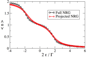
Figure 2: (Color online) Comparison of the projected NRG and full DM-NRG results for the total occupation of the dot for $\varepsilon=\varepsilon_{1}\equiv\varepsilon_{2}$ for couplings $v_{1}^{L}=0.33\,\sqrt{\Gamma}$, $v_{1}^{R}=0.37\,\sqrt{\Gamma}$, $v_{2}^{L}=0.42\,\sqrt{\Gamma}$ and $v_{2}^{R}=-0.46\,\sqrt{\Gamma}$. The Coulomb energy is $U=2\,\Gamma$, $\alpha=0.9\,\Gamma$ and $t=0.2\,\Gamma$.

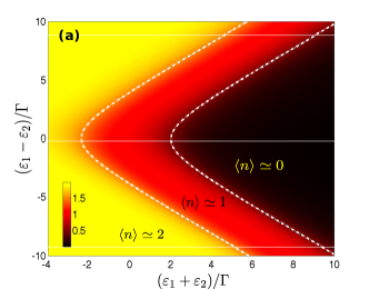
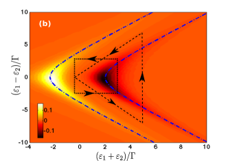
Figure 3: (Color online) (a) Density plot for the total occupation number in the $[\bar{\varepsilon},\Delta\varepsilon]$ plane for the same parameters as in Fig. 2. (b) Dimensionless spin field $\Gamma^{2}\,\mathbf{\Pi}_{L}^{(S)}(\bar{\varepsilon},\Delta\varepsilon)$ for the same parameters. The dashed black triangle indicates the pumping cycle used in Fig.  4. Fig. 1 shows the cycle indicated by dotted black lines. Dash-dotted blue lines denote the mixed valence regimes, where the total occupation is $\langle n\rangle=0.5$ ($\langle n\rangle=1.5$).

Results: To compute the pumping fields, we employed the density matrix NRG (DM-NRG) approach Bud (2008) to compute $\langle n\rangle$, and exploited the Friedel sum rule to construct $G_{D}(\omega=0)$ and the S-matrix as a function of $\varepsilon_{1}$ and $\varepsilon_{2}$ using Eq. (6). To check the validity of our projective approach, we also performed DM-NRG calculations for the unprojected Hamiltonian and determined the occupation $\langle n\rangle$ . The agreement is very good (see Fig. 2): the location as well as the shape of the charging steps are reproduced accurately by the projected Hamiltonian.

In Fig. 3, we present the spin pumping field, Eq. (3), as well as the occupation $\langle n\rangle$ as a function of $\bar{\varepsilon}$ and $\Delta\varepsilon$. Two strong resonances appear for $\Delta\varepsilon\approx 0$, precisely in the vicinity of the mixed valence regimes. The first resonance at $\bar{\epsilon}\approx\sqrt{\alpha^{2}+t^{2}}$ corresponds to the $n=0\leftrightarrow 1$ transition, and resembles very much to the resonance found in the non-interacting case Brosco et al. (2010). Encircling this first resonance corresponds to a cycle sketched in Fig. 1: (1) first one populates level $\varepsilon_{1}$ by pulling it below the Fermi level. Then, (2) exchanging $\varepsilon_{1}\leftrightarrow\varepsilon_{2}$ one changes the spin content of the lower level, $E_{-}$. (3) Finally, one empties the level by pulling it over the Fermi energy.

However, a surprising second antiresonance appears at $\bar{\epsilon}\approx\sqrt{\alpha^{2}+t^{2}}-U$. This antiresonance is associated with the transition $n=1\leftrightarrow 2$. It emerges solely as a consequence of strong Coulomb interactions, and cannot be explained within a non-interacting picture. It ”mirrors” the first resonance, but it carries just the opposite spin. This can be intuitively understood as follows: The doubly occupied level is a Kramers singlet and carries no spin. Therefore, the second electron entering the quantum dot must carry a spin opposite to the first one.

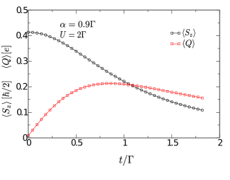
Figure 4: Pumped charge and spin per cycle as function of the hybridization $t$ of the two levels, as computed for the triangle-shaped cycle in Fig. 3.b. The couplings are fixed to $v_{1}^{L}=0.33\,\sqrt{\Gamma}$, $v_{1}^{R}=0.37\,\sqrt{\Gamma}$, $v_{2}^{L}=0.42\,\sqrt{\Gamma}$ and $v_{2}^{R}=-0.46\,\sqrt{\Gamma}$. $\langle S_{z}\rangle$ is measured in units of $\hbar/2$ and the pumped charge $\langle Q\rangle$ in units of e.

To characterize the strength of the observed resonances, we computed the total spin pumped through a cycle, $(\varepsilon_{1},\varepsilon_{2})=(0,0)\to(0,5\,\Gamma)\to(5\,\Gamma,0)\to(0,0)$ (triangle in Fig. 3). For optimal parameters, the total spin pumped can reach values of the order of $\sim\hbar/2$. The value of the pumped spin is almost independent of the Coulomb interaction as long as $U$ is sufficiently large. However, since the pumping originates from the large amplitude of the spin flip process during the avoided level crossing at $\varepsilon_{1}\approx\varepsilon_{2}$, its strength is relatively sensitive to the spin independent interlevel hybridization, $t$, which suppresses the amplitude of these spin flip processes, and gradually suppresses the pumped spin (see Fig. 4).

Our projective approach can easily be extended to the regime $\langle n\rangle\geq 2$ by means of an electron-hole transformation, which symmetry also allows us to determine the structure of the pumping fields in the whole parameter region (see Fig. 5): altogether we find two pairs of spin pumping resonances, two resonances corresponding to the charging of each Kramers degenerate level.

For generic couplings, $v_{j}^{r}$, spin pumping is also accompanied by charge pumping, which, however, may be strongly suppressed for special geometries. For a symmetrical device, e.g., with $v_{1}^{L}=v_{1}^{R}$ and $v_{2}^{L}=-v_{2}^{R}$ the charge field vanishes identically, and one obtains pure spin pumping, similar to the non-interacting case San-Jose et al. (2006).

Conclusions: In the present paper, we used the concepts of Fermi liquid theory to formulate low temperature spin pumping through an interacting many-body system in terms of the many-body S-matrix. We applied this formalism for a strongly interacting quantum dot with two gate-tuned levels, and showed that – due to the strong interactions – pumping field strong resonances and anti-resonances appear at every mixed valence transition, which can be used to pump purely electronically a spin of the order $\sim\hbar/\mathrm{cycle}$ in a controlled way.

Acknowledgments. We acknowledge useful discussions with Sylvia Kusminskiy and Jürgen König. This research has been supported by Hungarian Research Funds under grant Nos. K105149, CNK80991, TAMOP-4.2.1/B-09/1/KMR-2010-0002, by the UEFISCDI under French-Romanian Grant DYMESYS (ANR 2011-IS04-001-01 and Contract No. PN-II-ID-JRP-2011-1) and the EU-NKTH GEOMDISS project.

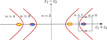
Figure 5: (Color online) Sketch of the occupation of the dot and the position of the spin pumping resonances.

References

- Žutić et al. (2004) I. Žutić, J. Fabian, and S. Das Sarma, Rev. Mod. Phys. 76, 323 (2004).
- Lee and Ramakrishnan (1985) P. A. Lee and T. V. Ramakrishnan, Rev. Mod. Phys. 57, 287 (1985).
- Brüne et al. (2011) C. Brüne, C. X. Liu, E. G. Novik, E. M. Hankiewicz, H. Buhmann, Y. L. Chen, X. L. Qi, Z. X. Shen, S. C. Zhang, and L. W. Molenkamp, Phys. Rev. Lett. 106, 126803 (2011).
- Kells et al. (2012) G. Kells, D. Meidan, and P. W. Brouwer, Phys. Rev. B 86, 100503 (2012).
- Brouwer et al. (2011) P. W. Brouwer, M. Duckheim, A. Romito, and F. von Oppen, Phys. Rev. B 84, 144526 (2011).
- Khaetskii and Nazarov (2000) A. V. Khaetskii and Y. V. Nazarov, Phys. Rev. B 61, 12639 (2000).
- Burkard et al. (1999) G. Burkard, D. Loss, and D. P. DiVincenzo, Phys. Rev. B 59, 2070 (1999).
- San-Jose et al. (2006) P. San-Jose, G. Zarand, A. Shnirman, and G. Schön, Phys. Rev. Lett. 97, 076803 (2006).
- Nowack et al. (2007) K. C. Nowack, F. H. L. Koppens, Y. V. Nazarov, and L. M. K. Vandersypen, Science 318, 1430 (2007).
- Brouwer (1998) P. W. Brouwer, Phys. Rev. B 58, R10135 (1998).
- Governale et al. (2003) M. Governale, F. Taddei, and R. Fazio, Phys. Rev. B 68, 155324 (2003).
- Brosco et al. (2010) V. Brosco, M. Jerger, P. San-José, G. Zarand, A. Shnirman, and G. Schön, Phys. Rev. B 82, 041309 (2010).
- Citro et al. (2003) R. Citro, N. Andrei, and Q. Niu, Phys. Rev. B 68, 165312 (2003).
- Sela and Oreg (2006) E. Sela and Y. Oreg, Phys. Rev. Lett. 96, 166802 (2006).
- Rojek et al. (2013) S. Rojek, J. König, and A. Shnirman, Phys. Rev. B 87, 075305 (2013).
- Aono (2003) T. Aono, Phys. Rev. B 67, 155303 (2003).
- Miller et al. (2003) J. B. Miller, D. M. Zumbühl, C. M. Marcus, Y. B. Lyanda-Geller, D. Goldhaber-Gordon, K. Campman, and A. C. Gossard, Phys. Rev. Lett. 90, 076807 (2003).
- Noziéres (1978) P. Noziéres, J. Phys. France 39, 1117 (1978).
- Borda et al. (2007) L. Borda, L. Fritz, N. Andrei, and G. Zaránd, Phys. Rev. B 75, 235112 (2007).
- Bud (2008) We used the open-access Budapest Flexible DM-NRG code, O. Legeza, C. P. Moca, A. I. Tóth, I. Weymann, G. Zaránd, arXiv:0809.3143 (2008), URL http://www.phy.bme.hu/~dmnrg/.