A scaling relation between merger rate of galaxies and their close pair count

Abstract

We study how to measure the galaxy merger rate from the observed close pair count. Using a high-resolution N-body/SPH cosmological simulation, we find an accurate scaling relation between galaxy pair counts and merger rates down to a stellar mass ratio of about 1:30. The relation explicitly accounts for the dependence on redshift (or time), on pair separation, and on mass of the two galaxies in a pair. With this relation, one can easily obtain the mean merger timescale for a close pair of galaxies. The use of virial masses, instead of stellar masses, is motivated by the fact that the dynamical friction time scale is mainly determined by the dark matter surrounding central and satellite galaxies. This fact can also minimize the error induced by uncertainties in modeling star formation in the simulation. Since the virial mass can be read from the well-established relation between the virial masses and the stellar masses in observation, our scaling relation can be easily applied to observations to obtain the merger rate and merger time scale. For major merger pairs (1:1-1:4) of galaxies above a stellar mass of $4\times 10^{10}\,h^{-1}{\rm M_{\odot}}$ at $z=0.1$, it takes about $0.31$ Gyr to merge for pairs within a projected distance of $20\,h^{-1}{\rm{kpc}}$ with stellar mass ratio of 1:1, while the time taken goes up to $1.6$ Gyr for mergers with stellar mass ratio of 1:4. Our results indicate that a single timescale usually used in literature is not accurate to describe mergers with the stellar mass ratio spanning even a narrow range from 1:1 to 1:4.

1. Introduction

Measuring merger rates of galaxies is crucial to studies of their growth history. For early-type galaxies, merger rates are decisive in quantifying their mass assembly history and size increase process. It determines whether the frequency of mergers is appropriate for the observed mass/size growth of the early-type galaxies (Nipoti et al., 2009, 2012; Chou et al., 2011; Bluck et al., 2012; Cimatti et al., 2012; Newman et al., 2012; McLure et al., 2013). For late-type galaxies, merger rates are important for understanding the episodic star formation, such as starbursts, which are induced and enhanced by gas-rich mergers (e.g. Hopkins et al., 2010; López-Sanjuan et al., 2010; López-Sanjuan et al., 2013).

In observational studies, merger rates are usually measured by counting the number of close galaxy pairs (e.g. Patton et al., 1997; Carlberg et al., 2000; Lin et al., 2004; Ryan et al., 2008; Berrier & Cooke, 2012). For such a measurement, a timescale has to be adopted (or assumed) for a close pair of galaxies to merge. The uncertainty associated with the merger timescale also represents the main uncertainty of the merger rate. In literature, the authors generally assume that galaxies within some projected distance (e.g., $20\,h^{-1}{\rm{kpc}}$) would merge in a constant timescale (around $0.5$ Gyr) after accounting for the projection effects (Patton et al., 2000, 2002; Bell et al., 2006; De Propris et al., 2007; Lin et al., 2004, 2008; Patton & Atfield, 2008). Kitzbichler & White (2008) checked these assumptions using semi-analytic catalogues derived from the Millennium Simulation (Springel, 2005). They found that the merger timescales in their results are typically larger by a factor of 2 than the constant timescale that is usually assumed. In their semi-analytical model, they traced the dynamics of satellite galaxies through following the subhalos that host them. Once the surrounding subhalo is tidally disrupted, the orphan galaxy is assumed to merge with its central galaxy after a dynamical friction time. It is parametrized as in Binney & Tremaine (1987), but multiplied by a fudge factor 2 (Kang et al., 2005; De Lucia & Helmi, 2008), to account for the underestimation of the dynamical friction times in Binney & Tremaine (1987)(Boylan-Kolchin et al., 2008; Jiang et al., 2008; Wetzel & White, 2010). The timescales on which close galaxies within a certain distance would merge, are therefore dependent on the dynamical times they adopted. Furthermore, the spatial positions of the orphan galaxies within the host halos cannot be accurately traced by the dark matter particles, which would affect the measurement of the count of close pairs. Moreover, Kitzbichler & White (2008) only considered major mergers with stellar mass ratios larger than 1:4. It is hence restricted to major merger studies, but not applicable for investigating galaxy growth through minor mergers, which are currently considered the most promising mechanism for the size evolution of early compact massive galaxies (Bezanson et al., 2009; Naab et al., 2009; Hilz et al., 2012; Oogi & Habe, 2013).

Lotz et al. (2008, 2010a, 2010b, 2011) analysed the timescales for mergers identified both with quantitative morphology and with close pairs using N-body/SPH simulations. For close pair timescales, they first studied individual merger pairs for several different projected separation criteria, seeking the dependence on mass ratio, gas fraction and orbits. To obtain the cosmologically-averaged merger timescale, they extracted the distributions of baryonic mass ratio and gas fraction from three cosmological- scale galaxy evolution models. Then they computed the average merger timescale by weighting the individual timescale with these distributions. They found that the timescale depends mainly on the outmost radius adopted to identify close pairs for major (1:1-1:4) mergers. However, as in Kitzbichler & White (2008), they did not consider the case of minor mergers for close pairs either. Later, Xu et al. (2012) combined the results in Lotz et al. (2010a) with the mass dependence and redshift dependence in Kitzbichler & White (2008), giving a description for timescales of major mergers with projected distance between $5\,h^{-1}{\rm{kpc}}$ and $20\,h^{-1}{\rm{kpc}}$ at redshift $z<1$.

In this work, we study the relation between the galaxy merger rate and number of close pairs using a cosmological N-body/SPH simulation. Compared with the work of Kitzbichler & White (2008), we trace the merger of galaxies with star particles, therefore we do not make any assumptions on the merger timescale and spatial positions of the orphan galaxies. We extend the series of work by Lotz et al to minor merges, and carefully examine the dependence of the merger rate on redshift and on pair separation. As the main result, we give a calibrated relation between the merger rate and the close pair count, where diverse factors are taken into account, including redshift, pair separation, and galaxy masses. This relation is applicable to both major and minor merger pair counts obtained in observations, up to a redshift of 2.

By passing, we would like to point out that two types of merger timescales are often used in the literature. One, used widely in theoretical modeling of galaxy formation, measures the time elapsed during which a satellite spirals into the central galaxy from the halo virial boundary (eg., Jiang et al., 2008; Boylan-Kolchin et al., 2008; Wetzel & White, 2010). The other, often used in observations, is the time duration after which a close pair of galaxies at a certain separation is expected to merge together. The timescale worked out in the paper is the latter which can be used to measure the merger rate with the observed galaxy pair counts.

2. Methods

We use an N-body/SPH simulation run with Gadget2 code (Springel, 2005) to calibrate the relation between galaxy merger rates and close pair counts. The simulation is the same as the one used in Jiang et al. (2008), which includes the implementation of radiative cooling, star formation and supernova feedback (Springel & Hernquist, 2003). The cosmological parameters are $\Omega_{\Lambda}=0.732$, $\Omega_{\rm m}=0.268$, $\Omega_{\rm b}$=0.044, $\sigma_{\rm 8}$=0.85, and the Hubble constant is $H_{\rm 0}=100h\,{\rm{km\,s^{-1}}}{\rm Mpc}^{-1}$ with $h=0.71$. The box is $100\,h^{-1}{\rm{Mpc}}$ on a side, with $512^{3}$ dark matter particles and $512^{3}$ gas particles. The resulting mass resolution for dark matter and gas particles is $4.6\times 10^{8}\,h^{-1}{\rm M_{\odot}}$ and $9.2\times 10^{7}\,h^{-1}{\rm M_{\odot}}$, respectively. The softening length of the gravitational force is roughly equivalent to a Plummer force softening of $4.5\,h^{-1}{\rm{kpc}}$ (comoving). The simulation starts from $z=120$, with an equal logarithmic scale factor interval of $\Delta\ln a=0.01$ between two consecutive outputs.

Dark matter halos are identified using the friends-of-friends (FOF) method, with a linking length of 0.2 times the mean inter-particle separation. By default, galaxies are identified with the friends-of-friends method, in which a linking-length of 0.025 times the mean inter-particle separation is applied to star particles. A galaxy merger is identified if the satellite galaxy and the central galaxy begin to have the same descendant at one snapshot, and continue to have the same descendant for the following four snapshots ($\geq$ half of the dynamical time of a halo). We use this criterion to ensure that the merger is a real one, but not just a close flyby.

As usual, two galaxy samples are defined in searching for close pairs. Galaxies in the primary sample are targeted to count their close neighbors from the secondary sample.

The volume merger rate can be written as

$$\Phi=n_{\rm 1}N_{\rm p}(<r_{\rm p})/T_{\rm mg},$$ (1)

where $n_{\rm 1}$ is the number density of the primary sample, and $N_{\rm p}(<r_{\rm p})$ is the mean number of close companions within a distance of $r_{\rm p}$ for each galaxy in the primary sample. $T_{\rm mg}$ is the average timescale for the satellite galaxies at $r_{\rm p}$ to merge with the central one. Here the primary sample (assumed to be central galaxies) and the secondary sample (assumed to be satellite galaxies) are exclusive to each other. Satellite-satellite pairs will be discussed in section 3.2.

The major mechanism that drives the merging of the two galaxies is the dynamical friction, which would exhaust the orbital energy of the satellite after a certain timescale. Therefore, we tentatively formulate the merging timescale $T_{\rm mg}$ in the form of dynamical friction timescale, $T_{\rm mg}\propto\frac{v_{\rm c}r_{\rm p}^{2}}{Gm_{\rm 2}\ln\Lambda}$ (Binney & Tremaine, 1987), where $v_{\rm c}$ is the circular velocity of the primary halo assuming an isothermal sphere, and $m_{\rm 2}$ is the satellite mass, which is supposed to be the total mass of the baryon and the dark matter that are bound in the satellite at the time of being observed. In simulations, it is usually called subhalo mass. In observations, however, it is not an easily accessible quantity. We will discuss more detailedly and look for appropriate proxies in the next section. Although the galaxy pairs are close in distance, some may have higher orbital energy that is equivalent to a larger circular radius than the considered radial extent. This effect has been absorbed into the timescale $T_{\rm mg}$.

If the satellite sample is statistically large enough, the influence of the circularity parameter would be averaged out. Therefore, the term related to the circularity parameter is not included here.

Considering $v_{\rm c}\approx\sqrt{\frac{Gm_{\rm 1,v}}{r_{\rm 1,v}}}$ in the primary halo, where the virial mass $m_{\rm 1,v}$ and virial radius $r_{\rm 1,v}$ are defined in terms of $200$ times the critical density of the universe, we have

$$T_{\rm mg}\propto\frac{{m_{\rm 1,v}}^{1/2}{r_{\rm p}}^{2}}{G^{1/2}m_{\rm 2}\ln\Lambda{r_{\rm 1,v}}^{1/2}}.\\$$ (2)

The Coulomb logarithm can be written as $\ln\Lambda\approx\ln\frac{b_{\rm max}}{b_{\rm min}}$, where $b_{\rm max}$ and $b_{\rm min}$ are the maximum and minimum impact parameters, respectively. When the satellite is initially outside the primary halo, and $b_{\rm max}$ approximates to the virial radius, we have $\ln\Lambda\approx\ln\frac{m_{\rm 1,v}}{m_{2,v}}$, if we take the virial velocity of the host halo as the initial velocity. Here $m_{1,v}$ and $m_{2,v}$ are the virial masses of the primary halo and the satellite halo, respectively, before the satellite enters the primary halo. In Jiang et al. (2008), they found that an alternative expression $\ln(1+\frac{m_{\rm 1,v}}{m_{2,v}})$ for the Coulomb logarithm performs better in explaining the time interval for the satellite between the time of entering the virial radius and merging with the central galaxy, mainly for the case of $m_{\rm 1,v}/m_{2,v}\leq 4$. However, for galaxy pairs in smaller distance, where satellites are well within the virial radius, both $b_{\rm max}$ and $b_{\rm min}$ are very uncertain (Hashimoto et al., 2003; Peñarrubia et al., 2004; Just et al., 2011). We therefore do not explore the explicit influence of $\ln\Lambda$, while tentatively integrating it into a constant coefficient in the following investigation.

Replacing $T_{\rm mg}$ in Equation (1) with Equation (2), we obtain

$$\Phi=A_{\ast}\frac{G^{1/2}m_{2}{r_{\rm 1,v}}^{1/2}n_{\rm 1}N_{\rm p}(<r_{\rm p})}{{m_{\rm 1,v}}^{1/2}{r_{\rm p}}^{2}}.\\$$ (3)

If Equation (3) holds, the coefficient $A_{\ast}$ would be a constant, regardless of galaxy masses and redshift. We will verify this relation by checking on the reciprocal of $A_{\ast}$,

$$\frac{1}{A_{\ast}}=\frac{1}{\Phi}\frac{G^{1/2}m_{2}{r_{\rm 1,v}}^{1/2}n_{\rm 1}N_{\rm p}(<r_{\rm p})}{{m_{\rm 1,v}}^{1/2}{r_{\rm p}}^{2}},\\$$ (4)

which would also be a constant if the connection between merger rates and close pair counts can be established by Equation (3).

3. Results

Equation (4) is obtained in the framework of dynamical friction, by assuming all merging pairs are central-satellite pairs. For satellite-satellite pairs that were central-satellite pairs before entering the primary halo, they may also merge. Jiang et al. (2010) showed that, this kind of merger is a similar process to that for central-satellite mergers. We will also examine if the relation formulated for central-satellite pairs applies to satellite-satellite pairs.

3.1. Central-Satellite Pairs

We know that one ruling factor of the dynamical process is the total bound mass of the satellite, including the baryonic mass and and the surrounding dark matter mass. As shown in Jiang et al. (2008), the merging timescale between the time of entering the virial radius and the final coalescence (type 1 in §1) can be established through the virial mass of the satellite. However, the total satellite mass varies at different stages of the merger. At the earlier stage when the satellite just enters the host halo, the dark matter mass dominates the satellite mass, and thus the merging timescale. While at the later phase of the merging, the dark matter is mostly stripped off, and the stellar mass of the satellite determines when they finally coalesce. Therefore, at a middle stage when the two galaxies are $\leq 100\,h^{-1}{\rm{kpc}}$ away, the satellite has partly lost its dark matter. The satellite mass $m_{2}$ would be difficult to determine, making it the most uncertain quantity in Equation (4). In this subsection, we will find a mass proxy which is observable and can be used for the relation (4).

3.1.1 Adopting Stellar Masses of Satellites

As a first try and as some previous works, we use the stellar mass $m_{\rm 2,s}$ to replace the satellite mass $m_{\rm 2}$ in Equation (4). The advantage to adopt the stellar mass is that it can be measured in observations. We set the radial extent $r_{\rm p}$ to correspond to $100/(1+z)\,h^{-1}{\rm{kpc}}$ at all redshifts, as a tradeoff between the statistics and the ’closeness’. In the left panel of Figure 1 we plot $\frac{1}{A_{\ast}}$ obtained from Equation (4) as a function of satellite stellar mass $m_{\rm 2,s}$ at a median redshift of $z=0.3$. Four samples of central galaxies are shown by different colored lines, with stellar masses of $30.0$ (black), $15.0$ (red), $7.5$ (green) and $4.0$ (blue), respectively, in unit of $10^{10}\,h^{-1}{\rm M_{\odot}}$. The corresponding halo masses lie in the range from $10^{12.4}\,h^{-1}{\rm M_{\odot}}$ to $10^{13.1}\,h^{-1}{\rm M_{\odot}}$. Galaxy pairs are selected down to a stellar mass ratio of $1:32$, except for the lowest $m_{\rm 1,s}$ for which the lowest $M_{\rm 2,s}$ is not included, as galaxies at this mass consist of only $\sim 30$ particles, and are subject to resolution effect. Error bars are plotted assuming Poisson fluctuations for merger pairs. The number of central galaxies being considered is 326, 505, 940 and 1275, respectively, as the primary mass is lowered. Close pair counts increase as the satellite mass decreases. For the $m_{\rm 1,s}=30.0\times 10^{10}\,h^{-1}{\rm M_{\odot}}$ sample, the number of close companions for each central galaxy $N_{\rm p}(<100/(1+z)\,h^{-1}{\rm{kpc}})$ ranges from less than 2.0 for the most massive satellites, to 11.0 for the satellites with the lowest mass. There is a tendency for $\frac{1}{A_{\ast}}$ to decrease as the central stellar mass decreases; $\frac{1}{A_{\ast}}$ changes by a factor of 3 for the range of $m_{\rm 1,s}$ being explored.

The fact that $\frac{1}{A_{\ast}}$ increases with $m_{\rm 1,s}$ implies that the stellar mass is not an optimal proxy for $m_{2}$. It is not unexpected as the dynamical friction timescale is determined by the total mass associated with the satellite. In this respect, subhalos are found and traced using a subhalo finder developed by Han et al. (2012). Here the method is extended to count in the baryonic particles. The right panel of Figure 1 shows a similar plot as that in the left panel, except that the total satellite mass is taken for $m_{\rm s}$. As expected, $\frac{1}{A_{\ast}}$ remains approximately constant for each case of central-satellite pairs, which confirms that the total satellite mass is responsible for the merging process. In fact, the behavior of $\frac{1}{A_{\ast}}$ showed in the left panel of Figure 1 can be well explained by Figure 2, which displays the accumulated distribution of retained mass fraction of subhalos at $z=0.3$ since being accreted. $M_{\rm sub}$ denotes the total self-bound mass of subhalos, including dark matter, stars and gas particles. $M_{\rm sub}^{acc}$ is $M_{\rm sub}$ at infall. The stellar mass ratio of the satellite inhabiting the subhalo to the central galaxy is above $1:30$. The virial masses of primary halos are similar to those hosting the central galaxies which are denoted with the same color in the left panel. Solid lines show results for subhalos at $100/(1+z)\,h^{-1}{\rm{kpc}}$ away from the halo center (also at $z=0.3$) . We can see that above $70\%$ of subhalos still retain over $20\%$ of their original mass before accretion. The retained mass is far more than the galaxy stellar mass residing in the center of the subhalo, given that the ratio of stellar mass to halo mass is at most a few percent (see, e.g., Behroozi et al., 2012). Even at a distance of $10-60\,h^{-1}{\rm{kpc}}$ which is widely used in literature, above $40\%$ of subhalos have a retained fraction of $\geq 20\%$ (the dashed lines). Thus, the total mass that is at work driving the merging outweighs the stellar mass of the galaxy.

Figure 2 also shows that the fraction of the mass (in terms of the subhalo mass at infall) retained by the satellites of a fixed stellar mass $m_{2,s}$ increases with the decrease of the host mass (from the black to the blue lines). This is because the same $r_{\rm p}$ corresponds to a smaller fraction of the halo size for a more massive host halo, and thus satellites in larger host halos have gone deeper in the potential well and have lost a larger fraction of dark matter, as indicated in Figure 2. Because of the dependence of the total mass retained by the satellites on the host mass, $\frac{1}{A_{\ast}}$ would show an increase with the increase of the host mass if $m_{2,s}$ is used for $m_{2}$ in Equation (4).

3.1.2 Accounting for Satellites’ Mass Loss

As discussed above, the total bound mass of the satellite (stellar mass $+$ retained dark matter mass) is what we need for $m_{2}$ in Equation (4). However, it is not feasible to directly measure the total mass for observed satellites in a large statistical sample. In order to obtain a convenient way of relating galaxy pair counts to merger rates, as a second try we replace $m_{2}$ with the total bound mass of the satellite.

The total bound mass of a satellite evolves when it spirals into the center of the host. The physical mechanism is the gravitational tidal stripping that reduces its bound mass. There exist numerous works which study the mass loss of subhalos (Tormen et al., 1998; Gao et al., 2004; Zentner et al., 2005; Diemand et al., 2007; Giocoli et al., 2008). For the purpose of our current work, we want to know how the mass loss of a subhalo depends on its position in the host halo in a statistical way. Han et al. (2012) showed that the size of subhalos, on average, is proportional to the radius where the subhalo density equals the background density. Under the assumption of an isothermal sphere for the halo, we can easily deduce that the retained mass of the satellite is proportional to $r_{\rm p}$. Therefore, the retained bound mass can be modeled as $m_{\rm sub}^{acc}\frac{r_{\rm p}}{r_{\rm 1,v}}$. However, it is hard to estimate the infall information from observations. We thus have a different try, in which the total bound mass at infall $m_{\rm sub}^{acc}$ is taken as the virial mass $m_{\rm 2,v}$ that a central galaxy with the same stellar mass as the satellite would have at the redshift being considered. Given that the relation between the halo mass and stellar mass evolves slowly with time (see, e.g., Wang & Jing, 2010; Behroozi et al., 2012; Yang et al., 2012), the two halo masses do not differ much. Now the retained bound mass is modeled as $m_{\rm 2,v}\frac{r_{\rm p}}{r_{\rm 1,v}}$.

On the other hand, the spherical collapse model of halos indicates $v_{\rm c}\propto H(z)r_{\rm 1,v}$, where $H(z)$ is the Hubble parameter at redshift $z$. Thus, we have $m_{\rm 1,v}\propto{r_{\rm 1,v}}^{3}\rho_{\rm crit}(z)\propto\frac{{v_{\rm c}}^{3}}{GH(z)}$, in which $\rho_{\rm crit}(z)$ is the critical density at redshift $z$. With this relation we have $v_{\rm c}=\sqrt{\frac{Gm_{\rm 1,v}}{r_{\rm 1,v}}}\propto[m_{\rm 1,v}GH_{\rm 0}E(z)]^{1/3}$. Replacing $m_{2}$ in Equation (3) with the bound mass $m_{\rm 2,v}\frac{r_{\rm p}}{r_{\rm 1,v}}$ and using the above relations, we have

$$\Phi=B_{\ast}\frac{m_{\rm 2,v}n_{\rm 1}N_{\rm p}(<r_{\rm p})[m_{\rm 1,v}GH_{\rm 0}E(z)]^{1/3}}{m_{\rm 1,v}r_{\rm p}}.\\$$ (5)

where $H_{\rm 0}$ is the Hubble parameter at $z=0$, and $E(z)=\Omega_{\rm\Lambda}+\Omega_{\rm m}(1+z)^{3}$. Figure 3 shows that, $\frac{1}{B_{\ast}}$ is nearly unchanged with respect to the primary galaxy mass and the satellite galaxy mass out to redshift $2$. This means that Equation (5) is valid to connect the number of close pairs to galaxy merger rate. We fit the $\log\frac{1}{B_{\ast}}$ values for each primary galaxy to a straight line with zero slope. The four fitted values are then averaged to give a final result at each redshift. The resulting mean value of $\log\frac{1}{B_{\ast}}$ is $-0.23$ at $z=0.3$, $-0.24$ at $z=0.8$, $-0.25$ at $z=1.3$, and $-0.21$ at $z=2.0$, respectively, shown as the dotted lines in the plot. These values are very close, giving a mean $\frac{1}{B_{\ast}}$ of $10^{-0.23}$ with fluctuations among different redshifts less than $10\%$. This indicates that the redshift dependence can be well accounted for by Equation (5).

Although the radial extent $r_{\rm p}$ varies at different redshifts in Figure 3, we explore the applicability of Equation (5) when different radial extent is adopted at the same redshift. Figure 4 shows results with $r_{\rm p}=50/(1+z)\,h^{-1}{\rm{kpc}}$ and $150/(1+z)\,h^{-1}{\rm{kpc}}$ at $z=0.3$. In both cases, $\frac{1}{B_{\ast}}$ is consistent with that obtained using $r_{\rm p}=100/(1+z)\,h^{-1}{\rm{kpc}}$ (dotted lines).

The above results show that Equation (5) can accurately describe the merger rate (at an accuracy $\sim 10\%$). This indicates that the average merger timescale for a pair of galaxies at a small separation $r_{\rm p}<150\,h^{-1}{\rm{kpc}}$ is

$$T_{\rm mg}=10^{-0.23}\frac{m_{\rm 1,v}}{m_{\rm 2,v}}[m_{\rm 1,v}GH_{\rm 0}E(z)]^{-1/3}r_{\rm p},$$ (6)

where the coefficient $\frac{1}{B_{\ast}}$ is already replaced by its mean value $10^{-0.23}$. The timescale linearly scales with the (physical) separation, and depends on the redshift through $E^{-1/3}(z)$. Its strong dependence on the halo masses $m_{\rm 1,v}$ and $m_{\rm 2,v}$ tells us that one must take into account the mass dependence when measuring the merger rate from the count of close pairs. Even for major mergers (which are routinely defined as the mergers with the stellar mass ratio above $1/4$), the timescale could change significantly.

3.2. Satellite-Satellite Pairs

In section 3.1, we have obtained a good relationship between the merger rate and close number counts within $100\,h^{-1}{\rm{kpc}}$ from central galaxies. We have considered the central-satellite pair which is the dominant merging pattern. However, the satellite-satellite merging pairs also exist, although they are minor in comparison to central-satellite pairs. We check in Figure 5 whether the scaling relation we have obtained still holds for satellite-satellite merging pairs. Dotted lines in each panel are the same as in Figure 3. At each redshift, most part of the four lines slightly lies above the dotted line. After applying the same fitting method as in Figure 3 to the data, the resulting amplitude is typically about $0.15$ dex higher than those for central-satellite pairs in Figure 3. This higher amplitude results from the lower merger rate for satellite-satellite pairs, compared to that for central-satellite pairs with the same masses (Jiang et al., 2010). At small separation ($\leq 100\,h^{-1}{\rm{kpc}}$), the contribution to pair counts from satellite-satellite pairs is at the level of $10\%$ (see, e.g., Yoo et al., 2006). In view of the small increase in $\frac{1}{B_{\ast}}$ for satellite-satellite pairs and the low fraction of such pairs, the influence of satellite-satellite pairs on the relation of merger rates and pair counts is expected to be very weak. We can therefore adopt the relation established only with central-satellite pairs.

3.3. Application to observations

So far, all the investigations were done in the 3-dimensional frame. In observations, what we usually get is the number count of galaxy pairs within a projected separation $r_{p}$ (e.g. from the correlation function measurement). Some of the close pairs in projection are foreground or background pairs which are separated beyond $r_{p}$ in the real 3-dimensional space. To account for the projection effect, one needs to introduce a correction factor $f_{\rm 3d}$ to convert a projected pair count ${N_{\rm p}}^{proj}$ to a 3-dimensional count, $N_{\rm p}=f_{\rm 3d}{N_{\rm p}}^{proj}$.

In Jiang et al. (2012), they found that the projected number density of satellites obeys a power-law form with the best-fit logarithmic slope of $-1.05$, and this profile is independent of both central galaxy luminosities and satellite luminosities. According to their Equation (8), for projected number of satellites within $r_{\rm p}$ which is equivalent to number of pairs in the central-satellite case, it has a fraction $f_{\rm 3d}=66\%$ within the real 3-dimensional $r_{\rm p}$. Halo masses in their sample are above $10^{12}{\rm M_{\odot}}$, spanning a wider range than the primary halo masses being considered here. The power-law slope for the satellite radial distribution is fixed out to the virial radius ($>300\,{\rm{kpc}}$). Therefore, this 3-dimensional fraction $f_{\rm 3d}$ is the same for all close pair cases ($<100\,h^{-1}{\rm{kpc}}$). For satellite-satellite pairs, we use the simulation to check whether $f_{\rm 3d}=0.66$ is also applicable or not. We project all galaxies in the simulation box on the $x-y$ plane while assuming the $z$-direction is along the line-of-sight, which is equivalent to selecting companions in a photometric survey with $\frac{\Delta z}{1+z}\leq 0.015$. We find that $f_{\rm 3d}=0.66$ are generally consistent with the simulation results, and thus can also be applied to satellite-satellite pairs.

According to $\Phi=n_{1}N_{\rm p}(<r_{\rm p})/T_{\rm mg}$, when the 3-dimensional pair count per unit volume $n_{1}N_{\rm p}(<r_{\rm p})$ is known, we can get the merger rate per unit volume by using Equation (6) for the merger timescale. But for observations, it is the pair count in projection $N_{\rm p}^{proj}$ that is more easily accessible. If $N_{\rm p}^{proj}$ is used to measure the merger rate, i.e. $\Phi=n_{1}N_{\rm p}^{proj}(<r_{\rm p})/T_{\rm mg}^{proj}$, the projection effect must be taken into account and the merger timescale becomes

$$T_{\rm mg}^{proj}(<r_{\rm p})=\frac{10^{-0.23}}{0.66}\frac{m_{\rm 1,v}}{m_{\rm 2,v}}[m_{\rm 1,v}GH_{\rm 0}E(z)]^{-1/3}r_{\rm p}.\\$$ (7)

Equation (7) offers us a method of computing the timescale for mergers between primary galaxies with stellar mass $m_{\rm 1,s}$ and secondary galaxies with stellar mass $m_{\rm 2,s}$ within a projected radius of $r_{\rm p}$. Besides the radial extent $r_{\rm p}$ and redshift $z$, there are two other input quantities in Equation (7): $m_{\rm 1,v}$ and $m_{\rm 2,v}$. $m_{\rm 1,v}$ is the median virial mass of isolated halos which host central galaxies of $m_{\rm 1,s}$ at redshift $z$. Similarly, $m_{\rm 2,v}$ is the median virial mass of isolated halos which host central galaxies of $m_{\rm 2,s}$ at redshift $z$. These virial masses, which are defined in terms of $200$ times the critical density, can be estimated from the relation between dark halo mass and central galaxy mass (e.g. Yang et al., 2003; Tinker et al., 2005; Mandelbaum et al., 2006; Wang et al., 2006; Yang et al., 2007; Zheng et al., 2007; Guo et al., 2010; Moster et al., 2010; Wang & Jing, 2010; More et al., 2011; Li et al., 2012; Behroozi et al., 2012; Yang et al., 2012; Velander et al., 2013). The error of measuring the merger rate through Equation (7) comes from the uncertainty of the close pair count and from the accuracy of the merger time scale. We estimate that the accuracy of our formula is at $10\%$ level. To reach a similar level of the merger rate measurement, one would need at least a few hundred of close pairs.

4. Discussions

In this section we will first discuss about the effect of modeling uncertainties of galaxies in the simulation. As we know, the baryonic physics governing galaxy formation and evolution is not fully understood yet, though the simulated galaxies already resemble closely those in the real Universe. As we have shown, the merger timescale depends on the masses of the satellite and the host halo, therefore it is important to check the ratio of the stellar mass to the dark matter halo mass of a galaxy, to see if the simulation is suitable for the study of the merger rate of galaxies. We show in Figure 6 the relation between the halo mass and stellar mass of the central galaxy for the lowest redshift case. Results are compared to those observed by Mandelbaum et al. (2006). It is clear that they are generally consistent, except for the highest mass bin where the halo mass is about $2.5$ times smaller in our simulation. This can be attributed to the gas overcooling in massive halos, which results from the lack of AGN feedback to a certain degree. Since most massive galaxies are central ones, the overcooling mainly affects the identification of merger remnants, while having little effect on the descending of satellites. As we emphasized in the end of §3.3, if we can find out the host halo mass of the central galaxies from observations (say from the halo occupation distribution method), we can compute the merger timescale accurately.

The gas overcooling problem of the most massive galaxies in the simulation should have negligible effect on our results for the merger time scales, because we do not explicitly use the stellar mass in the equations. This is further illustrated with a different identification method which will leads to a different correspondence between the halo mass and the galaxy stellar mass (green points with error bars in Figure 6 ). Here we use a smaller linking length ($b=0.0125$) when identifying galaxies. For a given host halo mass, the galaxy stellar mass is smaller than the galaxies identified with $b=0.025$ in the previous section. Because we use the correct dark halo mass for each galaxy in Equation (5), we would expect very little change from the case of $b=0.025$. This is shown in Figure 7, which shows that the change is indeed small when the new results are compared to the dotted lines which are the same as in Figure 3. The largest change happens at $z=2.0$, where $\frac{1}{B_{\ast}}$ is higher than that in Figure 3 by about $20\%$. Only the central core of a galaxy would be selected into a galaxy again after shortening the linking length. It makes galaxies more easily stripped of particles, thus delaying the merger identification or reducing identified merger events. This explains why $\frac{1}{B_{\ast}}$ is relatively higher here. The results reinforce the conclusion that the merger timescale is dominated by the gravitational process, as shown by Jiang et al. (2010) who found that even if the baryonic mass is halved in the simulation, the time needed for a satellite at the host virial radius to merge with the central galaxy generally changes at the level of $10\%$. We therefore expect that the merger timescale for close galaxy pairs would change at a similar level if the stellar mass changes by less than $2$ times.

Next we make a comparison with results from Kitzbichler & White (2008). We calculate $T_{\rm mg}^{proj}$ for galaxies more massive than $4\times 10^{10}\,h^{-1}{\rm M_{\odot}}$ within a projected distance of $100/(1+z)\,h^{-1}{\rm{kpc}}$ at $z=0.1$. Kitzbichler & White (2008) gives a timescale of $9.0$ Gyr for such mergers. Since their stellar mass ratio is between 1:1 and 1:4, we compute $T_{\rm mg}^{proj}$ accordingly, finding $T_{\rm mg}^{proj}$ is between $1.6$ Gyr and $8.2$ Gyr ($h=0.71$), corresponding to 1:1 mergers and 1:4 mergers respectively. The stellar mass is converted to halo mass using the relation between halo mass and central stellar mass established in Mandelbaum et al. (2006). The timescale computed according to Kitzbichler & White (2008) ($9.0$ Gyr) is only close to that for 1:4 mergers in our results. On the other hand, the merger timescales for the same galaxies but within projected $20\,h^{-1}{\rm{kpc}}$ are between $0.31$ Gyr (1:1) and $1.6$ Gyr (1:4), by assuming $T_{\rm mg}^{proj}$ is proportional to the outmost radius. These all indicate that a single timescale is not sufficient to describe mergers with stellar mass ratios in the range from 1:1 to 1:4. We need to consider the dependence of the timescale on both virial masses of the two galaxies.

5. Conclusions

Using a high-resolution N-body/SPH cosmological simulation, we have studied the relation between galaxy pair counts and merger rates. Our results indicate that galaxy merger rates can be inferred at an accuracy $\sim 10\%$ from the number of close pairs as shown by Equation (5). The equation gives explicit dependence on the bound masses of galaxies, on the pair separation and on the redshift. Equivalently, the merger timescale can be established for galaxy pairs with the physical separation less than $150\,h^{-1}{\rm{kpc}}$ down to a stellar mass ratio of $1:30$ out to redshift $2.0$.

Although stellar mass can be directly measured in galaxy surveys, the dynamical friction time scale is determined by the total bound mass surrounding the galaxies. By using the virial mass of both galaxies in the close pair and properly considering the mass loss of subhalos, we present an accurate scaling relation (Equation 7) for galaxy mergers within a projected distance $r_{\rm p}$. For this equation to be applied to real observations, the virial mass of the galaxies should be obtained with the techniques such as the halo occupation distribution method. The additional advantage of using the bound mass for the merger timescale is that our results are rather insensitive to the modeling details of galaxies in the simulation.

For major mergers (1:1-1:4) of galaxies above $4\times 10^{10}\,h^{-1}{\rm M_{\odot}}$ at $z=0.1$, estimated merger timescales ($r_{\rm p}<100\,h^{-1}{\rm{kpc}}$) based on Equation (7) spans a wide range from $1.6$ Gyr to $8.2$ Gyr ($h=0.71$), corresponding to 1:1 mergers and 1:4 mergers respectively. In contrast, the timescale given by Kitzbichler & White (2008) ($9.0$ Gyr) is only close to that for 1:4 mergers in our results. Our results indicate that a single timescale is not enough to describe mergers of stellar mass ratios even only from 1:1 to 1:4, and the dependence on the virial masses of the galaxies must be taken into account.

Although all the equations are formulated for central-satellite pairs, satellite-satellite merging can also be approximately described, with a typical deviation of $0.15$ dex for the normalizing factor. This is a consequence of relatively lower merger rates for satellite-satellite pairs. Our results for the satellite-satellite can be incorporated into an accurate modeling of the merger rate if the satellite fraction of galaxies is known (say, from HOD modeling (Zheng et al., 2007, e.g.)). Since the fraction of satellite-satellite pairs is low (at $\sim 10\%$ level), the influence of such pairs to the relation of merger rates and pair counts is expected to be very weak. The relation established with central-satellite pairs can therefore be applied to all galaxies pairs to a good approximation.

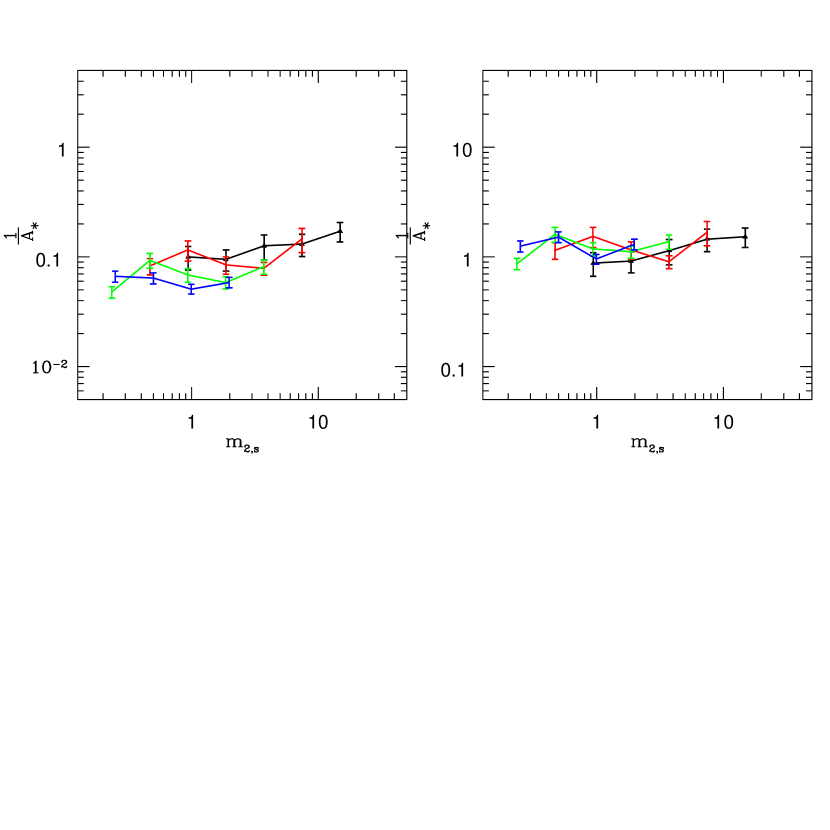
Figure 1.— Left: $\frac{1}{A_{\ast}}$ obtained according to Equation (4) when the stellar mass $m_{2,s}$ is used for the satellite mass. Only central-satellite pairs are included. Four colored lines show samples with central stellar masses of $30.0$ (black), $15.0$ (red), $7.5$ (green) and $4.0$ (blue), respectively, in unit of $10^{10}\,h^{-1}{\rm M_{\odot}}$. The outer radius corresponds to $100/(1+z)\,h^{-1}{\rm{kpc}}$. Error bars show the poisson fluctuations of the merging pairs. Right: Similar to the left panel, except that the total bound mass of the satellite is used in Equation (4).

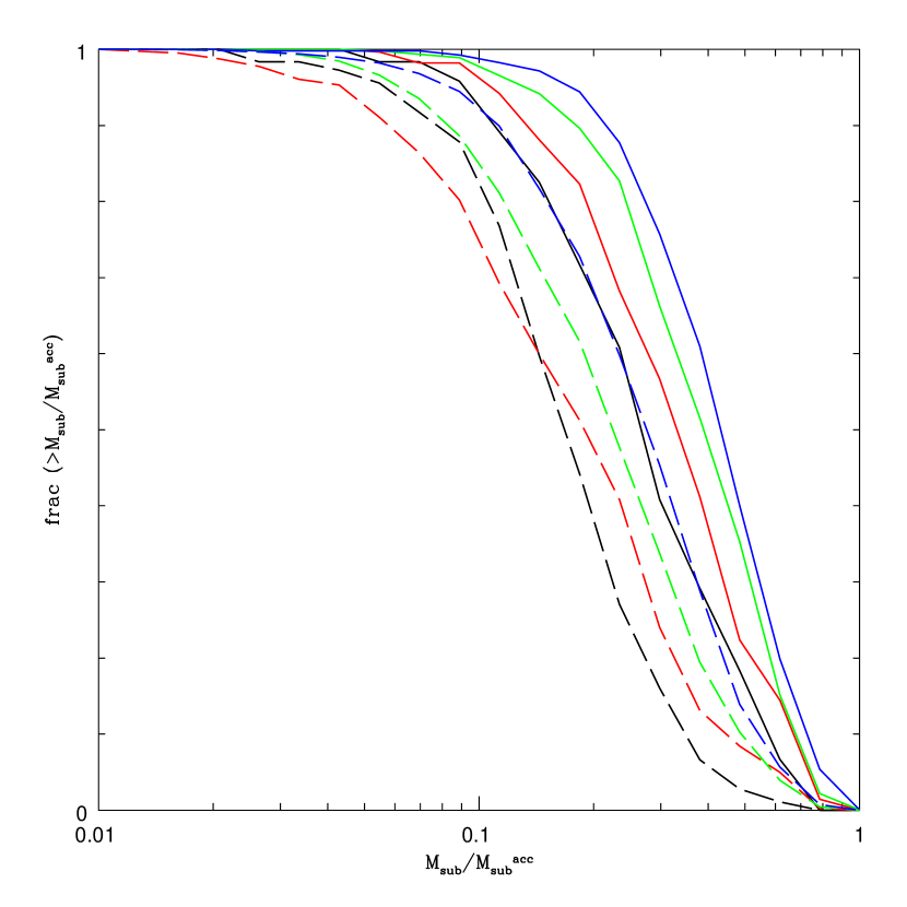
Figure 2.— Accumulated distributions of retained mass fraction of subhalos since accretion, for subhalos around $100/(1+z)\,h^{-1}{\rm{kpc}}$ ($z=0.3$) away from the halo center (solid lines), and those $10-60\,h^{-1}{\rm{kpc}}$ away from the halo center at $z=0.3$ (dashed lines). The virial masses of primary halos are similar to those hosting the central galaxies which are denoted with the same color in the left panel. The stellar mass ratio of the satellite inhabiting the subhalo to the central galaxy is above $1:30$.

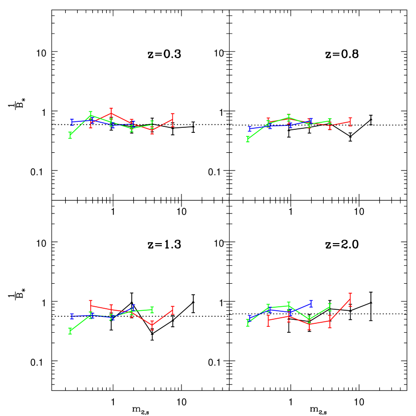
Figure 3.— Same as the left panel of Figure 1, but the virial mass for satellites is used (Equation 5). Results are shown in 4 redshifts as displayed in different panels. The dotted lines are the fitting results at each redshift, showing $\log 10(\frac{1}{B_{\ast}})=-0.23,-0.24,-0.25,-0.21$ respectively, as the redshift increases.

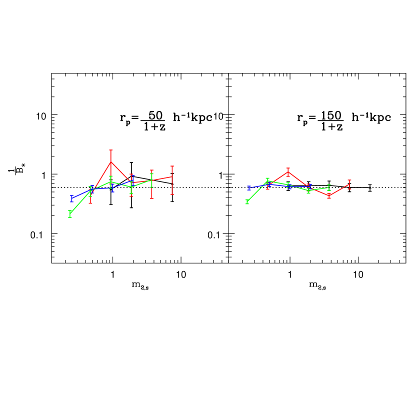
Figure 4.— Same as the upper left panel in Figure 3, but the outer radius corresponds to $50/(1+z)\,h^{-1}{\rm{kpc}}$ (left), and $150(1+z)\,h^{-1}{\rm{kpc}}$ (right).

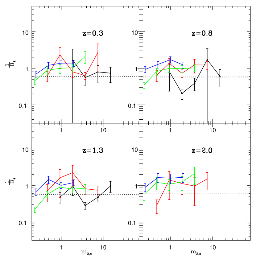
Figure 5.— Same as Figure 3, but for satellite-satellite pairs. The dotted lines are the same as in Figure 3.

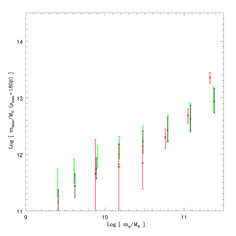
Figure 6.— Median halo mass as a function of its central stellar mass at $z=0.3$ (points with error bars showing $68.3\%$ interval), black for the default galaxy identification method (b=0.025) and green for b=0.0125. The bin width of the stellar mass is $0.3$ in logarithmic space. To compare with the results from Mandelbaum et al. (2006) (red points), we define halo mass here as that enclosed within the radius, where the overdensity is equal to 180 times the mean density.

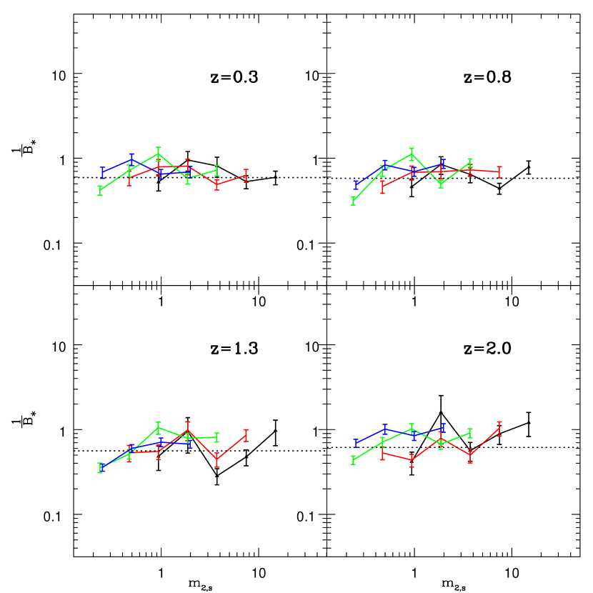
Figure 7.— Same as Figure 3, but galaxies are linked with a smaller linking length ($b=0.0125$). Dotted lines are the same as those in Figure 3.

References

- Behroozi et al. (2012) Behroozi, P. S., Wechsler, R. H., & Conroy, C. 2012, arXiv:1207.6105
- Bell et al. (2006) Bell, E. F., Phleps, S., Somerville, R. S., et al. 2006, ApJ, 652, 270
- Berrier & Cooke (2012) Berrier, J. C., & Cooke, J. 2012, MNRAS, 426, 1647
- Bezanson et al. (2009) Bezanson, R., van Dokkum, P. G., Tal, T., et al. 2009, ApJ, 697, 1290
- Binney & Tremaine (1987) Binney, J., & Tremaine, S. 1987, Princeton, NJ, Princeton University Press, 1987, 747 p.,
- Bluck et al. (2012) Bluck, A. F. L., Conselice, C. J., Buitrago, F., et al. 2012, ApJ, 747, 34
- Boylan-Kolchin et al. (2008) Boylan-Kolchin, M., Ma, C.-P., & Quataert, E. 2008, MNRAS, 383, 93
- Carlberg et al. (2000) Carlberg, R. G., Cohen, J. G., Patton, D. R., et al. 2000, ApJ, 532, L1
- Chou et al. (2011) Chou, R. C. Y., Bridge, C. R., & Abraham, R. G. 2011, AJ, 141, 87
- Cimatti et al. (2012) Cimatti, A., Nipoti, C., & Cassata, P. 2012, MNRAS, 422, L62
- De Lucia & Helmi (2008) De Lucia, G., & Helmi, A. 2008, MNRAS, 391, 14
- De Propris et al. (2007) De Propris, R., Conselice, C. J., Liske, J., et al. 2007, ApJ, 666, 212
- Diemand et al. (2007) Diemand, J., Kuhlen, M., & Madau, P. 2007, ApJ, 667, 859
- Gao et al. (2004) Gao, L., White, S. D. M., Jenkins, A., Stoehr, F., & Springel, V. 2004, MNRAS, 355, 819
- Giocoli et al. (2008) Giocoli, C., Tormen, G., & van den Bosch, F. C. 2008, MNRAS, 386, 2135
- Guo et al. (2010) Guo, Q., White, S., Li, C., & Boylan-Kolchin, M. 2010, MNRAS, 404, 1111
- Han et al. (2012) Han, J., Jing, Y. P., Wang, H., & Wang, W. 2012, MNRAS, 427, 2437
- Hashimoto et al. (2003) Hashimoto, Y., Funato, Y., & Makino, J. 2003, ApJ, 582, 196
- Hilz et al. (2012) Hilz, M., Naab, T., Ostriker, J. P., et al. 2012, MNRAS, 425, 3119
- Hopkins et al. (2010) Hopkins, P. F., Younger, J. D., Hayward, C. C., Narayanan, D., & Hernquist, L. 2010, MNRAS, 402, 1693
- Jiang et al. (2008) Jiang, C. Y., Jing, Y. P., Faltenbacher, A., Lin, W. P., & Li, C. 2008, ApJ, 675, 1095
- Jiang et al. (2012) Jiang, C. Y., Jing, Y. P., & Li, C. 2012, ApJ, 760, 16
- Jiang et al. (2010) Jiang, C. Y., Jing, Y. P., & Lin, W. P. 2010, A&A, 510, A60
- Just et al. (2011) Just, A., Khan, F. M., Berczik, P., Ernst, A., & Spurzem, R. 2011, MNRAS, 411, 653
- Kang et al. (2005) Kang, X., Jing, Y. P., Mo, H. J., Börner, G. 2005, ApJ, 631, 21
- Kitzbichler & White (2008) Kitzbichler, M. G., & White, S. D. M. 2008, MNRAS, 391, 1489
- Li et al. (2012) Li, C., Jing, Y. P., Mao, S., et al. 2012, ApJ, 758, 50
- Le Fèvre et al. (2000) Le Fèvre, O., Abraham, R., Lilly, S. J., et al. 2000, MNRAS, 311, 565
- Lin et al. (2004) Lin, L., Koo, D. C., Willmer, C. N. A., et al. 2004, ApJ, 617, L9
- Lin et al. (2008) Lin, L., Patton, D. R., Koo, D. C., et al. 2008, ApJ, 681, 232
- López-Sanjuan et al. (2010) López-Sanjuan, C., Balcells, M., Pérez-González, P. G., et al. 2010, ApJ, 710, 1170
- López-Sanjuan et al. (2013) López-Sanjuan, C., Le Fèvre, O., Tasca, L. A. M., et al. 2013, A&A, 553, A78
- Lotz et al. (2011) Lotz, J. M., Jonsson, P., Cox, T. J., et al. 2011, ApJ, 742, 103
- Lotz et al. (2010a) Lotz, J. M., Jonsson, P., Cox, T. J., & Primack, J. R. 2010a, MNRAS, 404, 575
- Lotz et al. (2010b) Lotz, J. M., Jonsson, P., Cox, T. J., & Primack, J. R. 2010b, MNRAS, 404, 590
- Lotz et al. (2008) Lotz, J. M., Jonsson, P., Cox, T. J., & Primack, J. R. 2008, MNRAS, 391, 1137
- Mandelbaum et al. (2006) Mandelbaum, R., Seljak, U., Kauffmann, G., Hirata, C. M., & Brinkmann, J. 2006, MNRAS, 368, 715
- McLure et al. (2013) McLure, R. J., Pearce, H. J., Dunlop, J. S., et al. 2013, MNRAS, 428, 1088
- More et al. (2011) More, S., van den Bosch, F. C., Cacciato, M., et al. 2011, MNRAS, 410, 210
- Moster et al. (2010) Moster, B. P., Somerville, R. S., Maulbetsch, C., et al. 2010, ApJ, 710, 903
- Naab et al. (2009) Naab, T., Johansson, P. H., & Ostriker, J. P. 2009, ApJ, 699, L178
- Newman et al. (2012) Newman, A. B., Ellis, R. S., Bundy, K., & Treu, T. 2012, ApJ, 746, 162
- Nipoti et al. (2009) Nipoti, C., Treu, T., Auger, M. W., & Bolton, A. S. 2009, ApJ, 706, L86
- Nipoti et al. (2012) Nipoti, C., Treu, T., Leauthaud, A., et al. 2012, MNRAS, 422, 1714
- Oogi & Habe (2013) Oogi, T., & Habe, A. 2013, MNRAS, 428, 641
- Patton & Atfield (2008) Patton, D. R., & Atfield, J. E. 2008, ApJ, 685, 235
- Patton et al. (2000) Patton, D. R., Carlberg, R. G., Marzke, R. O., et al. 2000, ApJ, 536, 153
- Patton et al. (2002) Patton, D. R., Pritchet, C. J., Carlberg, R. G., et al. 2002, ApJ, 565, 208
- Patton et al. (1997) Patton, D. R., Pritchet, C. J., Yee, H. K. C., Ellingson, E., & Carlberg, R. G. 1997, ApJ, 475, 29
- Peñarrubia et al. (2004) Peñarrubia, J., Just, A., & Kroupa, P. 2004, MNRAS, 349, 747
- Ryan et al. (2008) Ryan, R. E., Jr., Cohen, S. H., Windhorst, R. A., & Silk, J. 2008, ApJ, 678, 751
- Scannapieco et al. (2012) Scannapieco, C., Wadepuhl, M., Parry, O. H., et al. 2012, MNRAS, 423, 1726
- Springel (2005) Springel, V. 2005, MNRAS, 364, 1105
- Springel & Hernquist (2003) Springel, V., & Hernquist, L. 2003, MNRAS, 339, 312
- Tinker et al. (2005) Tinker, J. L., Weinberg, D. H., Zheng, Z., & Zehavi, I. 2005, ApJ, 631, 41
- Tormen et al. (1998) Tormen, G., Diaferio, A., & Syer, D. 1998, MNRAS, 299, 728
- Velander et al. (2013) Velander, M., van Uitert, E., Hoekstra, H., et al. 2013, arXiv:1304.4265
- Wang & Jing (2010) Wang, L., & Jing, Y. P. 2010, MNRAS, 402, 1796
- Wang et al. (2006) Wang, L., Li, C., Kauffmann, G., & De Lucia, G. 2006, MNRAS, 371, 537
- Wetzel et al. (2008) Wetzel, A. R., Schulz, A. E., Holz, D. E., & Warren, M. S. 2008, ApJ, 683, 1
- Wetzel & White (2010) Wetzel, A. R., & White, M. 2010, MNRAS, 403, 1072
- White (2001) White, M. 2001, A&A, 367, 27
- Xu et al. (2012) Xu, C. K., Zhao, Y., Scoville, N., et al. 2012, ApJ, 747, 85
- Yang et al. (2003) Yang, X., Mo, H. J., & van den Bosch, F. C. 2003, MNRAS, 339, 1057
- Yang et al. (2007) Yang, X., Mo, H. J., van den Bosch, F. C., et al. 2007, ApJ, 671, 153
- Yang et al. (2012) Yang, X., Mo, H. J., van den Bosch, F. C., Zhang, Y., & Han, J. 2012, ApJ, 752, 41
- Yoo et al. (2006) Yoo, J., Tinker, J. L., Weinberg, D. H., et al. 2006, ApJ, 652, 26
- Zentner et al. (2005) Zentner, A. R., Berlind, A. A., Bullock, J. S., Kravtsov, A. V., & Wechsler, R. H. 2005, ApJ, 624, 505
- Zheng et al. (2007) Zheng, Z., Coil, A. L., & Zehavi, I. 2007, ApJ, 667, 760