Long Term Spectral Evolution of Tidal Disruption Candidates Selected by Strong Coronal Lines

Abstract

We present results of follow-up optical spectroscopic observations of seven rare, extreme coronal line emitting galaxies reported by Wang et al. (2012) with Multi-Mirror Telescope (MMT). Large variations in coronal lines are found in four objects, making them strong candidates of tidal disruption events (TDE). For the four TDE candidates, all the coronal lines with ionization status higher than [Fe VII] disappear within 5-9 years. The [Fe VII] faded by a factor of about five in one object (J0952+2143) within 4 years, whereas emerged in other two without them previously. A strong increment in the [O III] flux is observed, shifting the line ratios towards the loci of active galactic nucleus on the BPT diagrams. Surprisingly, we detect a non-canonical [O III]$\lambda$5007/[O III]$\lambda$4959$\simeq$2 in two objects, indicating a large column density of O²⁺ and thus probably optical thick gas. This also requires a very large ionization parameter and relatively soft ionizing spectral energy distribution (e.g. blackbody with $T<5\times 10^{4}$ K). Our observations can be explained as echoing of a strong ultraviolet to soft X-ray flare caused by tidal disruption events, on molecular clouds in the inner parsecs of the galactic nuclei. Re-analyzing the SDSS spectra reveals double-peaked or strongly blue-shouldered broad lines in three of the objects, which disappeared in the MMT spectra in two objects, and faded by a factor of ten in 8 years in the remaining object with a decrease in both the line width and centroid offset. We interpret these broad lines as arising from decelerating biconical outflows. Our results demonstrate that the signatures of echoing can persist for as long as ten years, and can be used to probe the gas environment in the quiescent galactic nuclei.

1 Introduction

Stellar and gaseous kinematics suggests that most galaxies harbor central supermassive black holes (SMBH) and that the SMBH masses are well correlated with the stellar masses or velocity dispersions of the galactic bulges (e.g. Kormendy & Richstone 1995; Magorrian et al. 1998; Ho 1998; Merritt & Ferrarese 2000; Gebhardt et al. 2000). When a star in the galactic nucleus accidentally passes within the tidal disruption radius of the massive black hole ($r_{p}<R_{T}\simeq R_{*}(M_{\rm BH}/M_{*})^{1/3}$, Hills 1975), it is torn apart by the tidal force of the black hole. About half of the stellar debris is ejected and the rest falls back towards the black hole, causing a bright flare lasting for a few months to years (Rees 1988; Ayal et al. 2000). For a black hole of mass between $10^{7}\ M_{\sun}$ and $10^{8}\ M_{\sun}$ and a solar-type star, the peak luminosity will be sub-Eddington ($L_{Edd}=1.3\times 10^{38}(M_{\rm BH}/M_{\sun}){\rm erg\ s}^{-1}$). For less massive black hole ($M_{\rm BH}<10^{7}\ M_{\sun}$), the rate of fall back initially exceeds the Eddington accretion rate, likely launching strong outflows. The spectra of the super-Eddington accretion tori and outflows are still uncertain, but when the fallback rate is below the Eddington rate, the gas is accreted onto the black hole via a thin disk and its radiation peaks in the UV to soft X-ray bands.

Besides UV and soft X-ray continuum flares, variable broad and narrow emission lines may be also seen in the spectra. Part of the UV and X-ray light may be reprocessed by the outflows or unbounded debris, giving rise to the broad emission lines (Bogdanović et al. 2004; Strubbe & Quataert 2009; Wang et al. 2011, hereafter W11; Gezari et al. 2012). The same UV and X-ray sources may also ionize the cold circum-nuclear interstellar medium (ISM), producing high ionization narrow lines (Ulmer 1999; Komossa et al. 2008; Wang et al. 2011, 2012). Broad lines are expected to follow the continuum variations closely because they are produced in a region very close to the continuum source. Narrow lines should also be variable, but on a longer time scale due to the response of ISM material further away to the continuum flare (light echoing). In particular, the high-ionization narrow lines which vary on time scales of years are unique features for the light echo of tidal disruption event (TDE), that distinguishes it from active galactic nuclei (AGNs), which possess narrow line regions (NLRs) of sizes from $10^{2}$ to $10^{3}$ pc. Because gas at large scale will have little response to the continuum flare on time scales of months to years, we may expect to observe only the spectrum from the very inner region of the NLR, which is likely dominated by high ionization lines, while low ionization lines from normal NLR is weak.

Wang et al. (2012, hereafter W12) carried out a systematic search for extreme coronal line emitters (ECLEs) in the spectroscopic samples of galaxies and low redshift quasars from the Sloan Digital Sky Survey (SDSS) Data Release 7 (DR7), following the initial results of detecting variable narrow lines in two ECLEs (Komossa et al. 2008, 2009; W11). They identified a sample of seven galaxies that show extremely strong coronal lines from [Fe X] up to [Fe XIV]. Traditional narrow-line diagnostics suggested they are non-active, and half of the sample show broad emission lines of complex profiles. Also the sample is split into low and high ionization subclasses according to the detection or non-detection of [Fe VII]. W12 showed that these lines are formed in a photo-ionized gas, and argued that ECLEs are most likely the light echoes of a tidal disruption flare based on energetics considerations. Most these galaxies are intermediate luminosity disk galaxies with small bulges. If all these sources turn out to be TDE, then the rate of such TDE is expected around a few times $10^{-5}$ per galaxy per year for galaxies in the absolute magnitudes around $-21.3<M_{i}<-18.9$.

However, there are some further questions left from previous studies. First, optical follow-ups were carried out for only two of the seven objects. It remains to be verified whether the rest of the sample also show the same variation trends. Second, the long term evolution of the emission lines is not known. On what time scale do coronal lines disappear? Are there any other special features in the later stage of evolution that can be used to identify such events on long time scales? With these questions, we initiated spectroscopic follow-up observations with the Multi-Mirror telescope (MMT) to characterize the spectral signatures at late phases of evolution. In this paper we will present an analysis of the follow-up MMT spectroscopic observations. The paper is organized as follows. We present the observations and data reduction in §2 and results on the spectral evolution in §3. We discuss the implication of these results in §4. Throughout the paper, we will adopt a $\Lambda$-CDM cosmology with $H_{0}=71{\rm km\ s}^{-1}\ {\rm Mpc}^{-1}$, $\Omega_{M}=0.28$ and $\Omega_{\Lambda}=0.72$.

2 Observations and Data Reduction

We observed all seven targets with the Blue Channel Spectrographs mounted on the Multi-Mirror Telescope (MMT) on December 26, 2011. The log of the observations is given in Table 1. During the observation, the typical seeing was 0$\farcs$8 and we adopt a long slit with 1$\arcsec$ width. The slit is centered on the galactic nuclei and orientated at the parallactic angle. We took exposures of all seven targets for 900s with 500 gpm grating, centering at 6000Å. This setting results in a spectral resolution $R=\lambda/\Delta\lambda=1430$ and a wavelength coverage from 4430Å to 7560Å. Unfortunately, the slit was not properly placed on the center of the galaxy for SDSS J1241+4426, thus we will ignore the red part of spectrum for this object. We also obtained the blue portion of spectra for five objects, including SDSS J0748+4712, SDSS J0938+1353, SDSS J0952+2143, SDSS J1055+5637, and SDSS J1241+4426 using 800 gpm grating, centered at 4100Å, and an exposure time of 900s for each. The latter gives a spectral resolution of 1730 and a wavelength coverage from 3100Å to 5100Å. Three and one KNPO standard stars were observed using the same settings as 500 gmp and 800 gmp during the observation for flux calibration, and 7 and 5 He-Ne-Ar lamp spectra with g500 and g800 grism sets were taken for the wavelength calibration. The raw two-dimension data reduction and spectral extraction were accomplished using standard routines in IRAF. To extract the nuclear spectra, we used the APALL task and choosed an aperture of 3$\arcsec$. We also extract the spectra with an aperture of 1$\arcsec$, all high ionization lines including coronal lines, [O III] and He II$\lambda$4686 are almost the same, so must come from the center 1$\arcsec$ region. We carried out the wavelength and flux calibration using the spectra of a He-Ne-Ar lamp and those of the standard stars, respectively. When applying different standard stars for flux calibration taken with 500 gpm, the spectra of the same object were consistent with each other within 5%. Thus, we take the medians as our final results. After the flux calibration, the blue and red spectra of the same object taken with the two gratings are consistent with each other within 8% in the overlapping region, indicating small uncertainty in the flux calibration. Then we rescale the blue part spectrum to match the red one, and then combine them. We estimate the spectral resolution by measuring the width of emission lines in the spectrum of He-Ne-Ar lamp. For 500 gpm grating and 800 gpm grating, their typical values are 90 km s^-1 and 69 km s^-1.

3 Results

3.1 Comparison between SDSS and MMT spectra

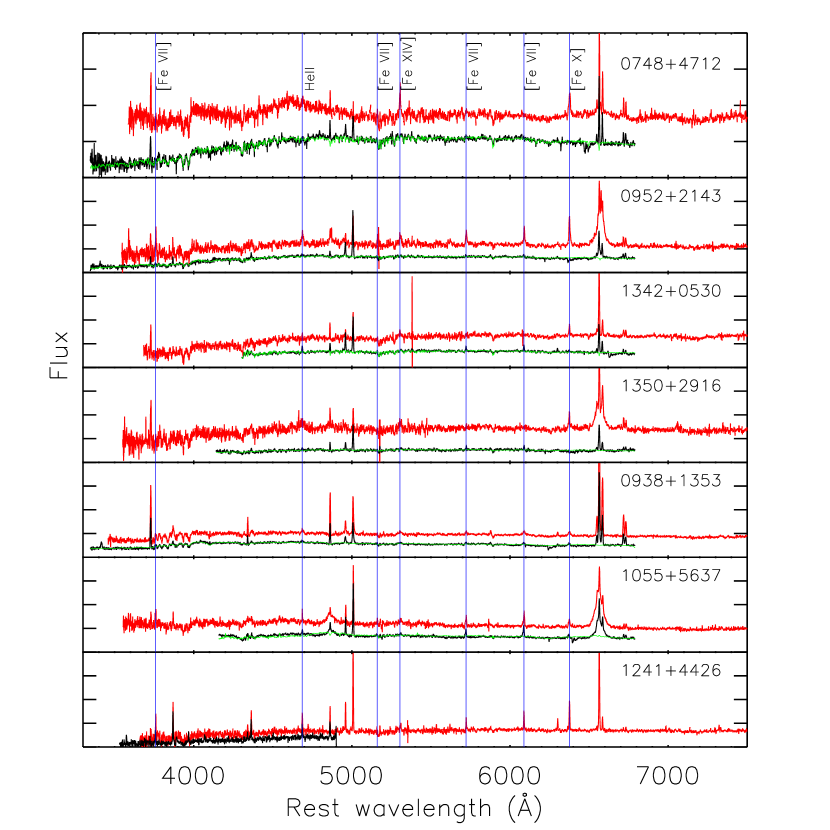
Figure 1: MMT(black) and SDSS(red) spectra of seven extreme coronal line emitters from W12. Continuum fit are plotted in green. Coronal lines and He II$\lambda$4686 are marked in blue. The spectra have been shifted in vertical direction for clarity.

The MMT spectra are shown in Figure 1. For comparison, we also overlay the SDSS spectra taken 5-9 years ago. Note that the SDSS spectra were taken using a larger aperture, a circle of 3$\farcs$0 in diameter, than ours, in 1$\farcs$0 $\times$ 3$\farcs$0 region, so they contain more light from the host galaxy than our MMT spectra. As such the low-ionization narrow lines from the extended star-formation regions may be significantly smaller in the MMT spectra, along with the starlight; while we do not expect that a significant coronal lines come from the extended region. Therefore, coronal lines will not be significantly affected by the aperture effect.

An initial check of the Figure 1 suggests two different variability trends for coronal lines. In four of seven objects, the high-ionization coronal lines [Fe X]$\lambda$6376-[Fe XIV]$\lambda$5304 completely disappeared in the MMT spectra, while for other three objects J0938+1353, J1055+5637 and J1241+4426, the MMT spectra are similar to the SDSS ones with strong high-ionization coronal lines. For J1241+4426, although we failed to obtain the red portion spectrum of the galactic center, we find that [Fe VII]$\lambda$3759 and [Ne III]$\lambda$3896 lines are prominent and do not show significant variation in the blue portion of the spectrum. Therefore, the latter three objects seem to be AGNs. The broad Balmer lines, Fe II and the non-stellar continuum remain very prominent in J1055+5637, thus it is a type 1 Seyfert galaxy. Note that J1055+5637 is the only object in W11 with narrow- line ratios located in the AGN regime in all three BPT diagrams. J0938+1353 shows fairly broad coronal and high ionization lines, superposing on strong, much narrower, low ionization lines, which come clearly from star-formation regions. We suspect that coronal lines and high ionization lines are from an obscured AGN. Thus it is likely a composite of a Seyfert 2 nucleus with star-formation regions but its true nature remains mysterious as coronal lines are not usually seen in composite type galaxies. Alternatively, the coronal lines may be related to tidal disruption of a giant star by a massive black hole, which produces a much longer lasting flare than of tidal disruption of a main sequence star. The latter scenario can be tested by future spectroscopic follow-up observations. We will focus only on the four variable objects in the late analysis.

3.2 Continuum Modeling and Variability

In this subsection we will model the continuum and examine the contribution of potential non-stellar continua in the SDSS spectrum. W12 found that four of the seven objects show flux variations between SDSS photometric and spectral observations, including the AGN J1055+5637. For two objects without [Fe VII] lines, they were brighter during the spectroscopic observations than during the photometric observation, indicating that there is a non-stellar continuum in J0748+4712 and J1350+2916 spectra, while it is difficult to assess the case in J0952+2143. If TDE is responsible for the continuum variability, any non-stellar continuum emission would be very weak after 5-9 years even if it existed during the SDSS spectroscopic observations. Indeed, in all MMT spectra, the continua are dominated by starlight. Therefore, the continua in the MMT spectra can be used as first- order templates for the stellar light in the SDSS by ignoring the radial gradients of stellar populations.

In order to get the starlight spectrum beneath the emission lines and also beyond the MMT spectral coverage, we fit the MMT spectra with a combination of 6 independent components (ICs) templates derived from the stellar populations (BC03) with Ensemble Learning Independent Component Analysis. Previous tests show that such extrapolation is reliable (see Lu et al. 2006 for detail). In practice, the continuum fit to a narrow wavelength coverage (4430Å to 7560Å) of the MMT spectrum of J1350+2916 can match its SDSS spectrum (wavelength coverage from 3700Å to 8500Å) well. During the fitting we mask all prominent emission lines, and convolve the templates with a Gaussian kernel and shift in redshift to match the width and the centroid of the absorption lines. The fits with 6 ICs are shown also in Figure 1.

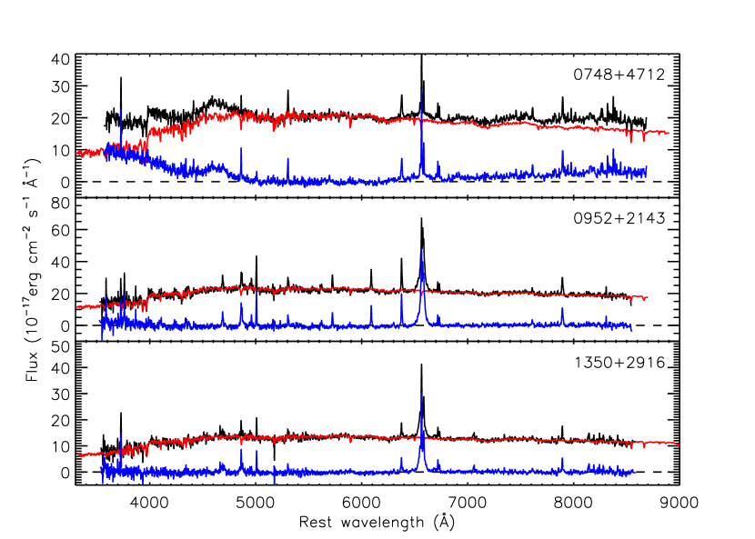
Figure 2: SDSS spectra of J0748+4712, J0952+2143, J1350+2916 (black) and scaled up MMT spectra’s 6ICs model (red) and the residuals of the substraction (blue). Both the spectra and models are smoothed by 3 pixels.

Keeping in mind that different amounts of the starlight lie within the apertures, we rescale the starlight models of J0748+4712, J0952+2143 and J1350+2916 derived from the MMT spectra to match their SDSS ones by minimizing the residuals in the stellar absorption lines. This yields the fit in Figure 2. Overall, the stellar absorption lines in the SDSS spectra are fitted very well, suggesting that this approach is feasible. A non-stellar continuum is required to be present in only SDSS J0748+4712. This provides an independent confirmation to the continuum variability analysis, further it also gives an estimate of the non-stellar continuum spectrum. Note this is much less model dependent than the spectral decomposition method using a combination of starlight plus a power-law or black-body fit in W11. We will describe the individual object below.

For J0748+4712, its SDSS spectrum shows strong non-stellar emission and three broad bumps around 4050, 4600 and 6560Å (see W11). The scaling factor of the star-light in the SDSS spectrum is 1.35. After subtracting the stellar light spectrum, the differential spectrum is a smooth continuum plus several broad bumps and narrow emission lines (Figure 2). One noticeable difference from W11 is that there is no broad feature around 4050Å, suggesting it was due to imperfect subtraction of stellar light in W11. The continuum is blue, but there is also a hint of curvature in the non-stellar spectrum. The latter is consistent with the variability analysis in W12 that the amplitudes appears larger in $g$ and $i$-bands than in $r$ band. But we cannot rule out the possibility that there is an additional old stellar population in the SDSS spectrum. If the curvature is confirmed, the non-stellar continuum may consist of two components, e.g., a disk component and a reprocessed outflow component.

It was reported that J0952+2143 also has a non-stellar continuum in the SDSS spectrum (Komossa et al 2009). These authors fitted the SDSS spectrum with a single simple stellar population plus a black-body emission. Our analysis does not confirm this. The SDSS continuum can be fitted very well with a scaled up MMT spectrum, therefore, a non-stellar component is not needed. For J1350+2916, W12 found that there is 3$\sigma$ evidence for brightening in the $g$ band between SDSS photometric and spectroscopic observations. Our analysis does not require a non-stellar component in this case. However, for this object, the MMT spectrum does not cover the 4000Å break or blueward of it, which is crucial to the detection of non-stellar component, because a non-stellar continuum is most prominent in short band and also the 4000Å break provides strong constraints on the scale of the stellar component.

3.3 Broad Emission Line Variability

Three of the four objects displayed prominent broad H$\alpha$, H$\beta$ or He II$\lambda$4686 lines in their SDSS spectra. Broad Balmer emission lines in J0952+2143 and J1350+2916 displayed double horns with separations between 2000 – 3000 km s^-1(see Komossa et al. 2008; W12). The FWHMs of these lines are 2100 and 2600 km s^-1, respectively. J0748+4712 showed two strong and broad (several hundred Å) bumps peaked around 4600 and 6560Å. The broad bump at 4600Å was interpreted as blue-shifted He II by W11. With the more reliable starlight subtraction here, this line also seems double peaked with the red peak close to the rest frame of He II while the blue peak at $-8,000$ km s^-1, although the signal to noise ratio is still a bit low. It is hard to attribute the blue peak to the contamination of another broad line as there is no strong lines expected in this wavelength range. Although the double peaks are not evident in the broad H$\alpha$ due to its weakness, the data are consistent with this. Thus, broad lines in all three TDE candidates show double peaked profiles. We have fitted the narrow H$\alpha$ and [N II] double lines with three narrow Gaussians and use a broad Gaussian to estimate the broad component of H$\alpha$ line. H$\alpha$ is detected with a flux of 2.1$\times 10^{-15}$erg cm^-2 s^-1. This gives a He II/H$\alpha$ ratio of 3.3.

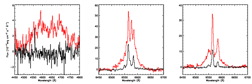
Figure 3: Broad bump around 4600Å in J0748+4712 (left panle,smoothed by 3 pixals) and H$\alpha$ regions of J0952+2143 (middle panel) and J1350+2916 (right panel). MMT spectra are plotted in black and SDSS spectra are plotted in red, all the spectra have been continuum substracted.

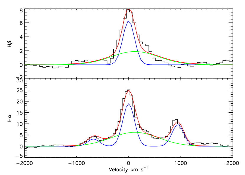
Figure 4: J0952+2143’s H$\alpha$ (low pannel) and H$\beta$ (up pannel) line profiles(black) in MMT spectrum. Normal narrow component fit is ploted in blue, redshift broad component is ploted in green. Model sum is plotted in red.

These broad bumps in J0748+4712 and double horns in J0952+2143 and J1350+2916 disappeared in the MMT spectra (Figure 3). Only very weak broad H$\alpha$ and H$\beta$ lines can be spotted in the MMT spectrum of J0952+2143 (middle panel of Figure 3 and figure 4). Any broad lines, if present, must be below the detection limits in the other two objects.

To measure the broad emission lines in J0952+2142, we fit the continuum subtracted spectra using Gaussians (Figure 4). All narrow lines show symmetric profiles. The H$\alpha$ and H$\beta$ lines display an additional redshifted broad component. Each symmetric narrow line is fitted with a Gaussian, while one more Gaussian component is added for the redshifted broad component of each Balmer line. H$\alpha$ and H$\beta$ are fitted, with the widths and centroids of each component locked. The line flux are listed in table 2. The broad component is redshifted by about 120 km s^-1 relative to the systematic velocity and has an FWHM of 620$\pm$45 km s^-1. It could be the relic of the fading broad Balmer lines seen in the SDSS and NTT spectra that was described in Komossa et al. (2008 & 2009). In those two spectra, which were taken on December 30, 2005 and Feb 6, 2008, the broad Balmer components had redshifts of 560 km s^-1 and 270 km s^-1, and FWHMs of 2100km s^-1 and 1500km s^-1. The line flux in the MMT spectrum is only 9% of that in SDSS spectrum and 25% in NTT spectrum.

3.4 Coronal Line Variability

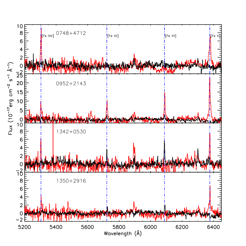
Figure 5: Coronal line of four TDE targets. From top to bottom: J0748+4712, J0952+2143, J1342+0530, J1350+2916. (black: MMT spectra, red: SDSS spectra)

Figure 5 compares the coronal line spectra, after subtracting the continuum of MMT spectra from those of the SDSS spectra over the wavelength range from 5200Å-6450Å, covering coronal lines [Fe VII], [Fe X]$\lambda$6376 and [Fe XIV]$\lambda$5304. The one Gaussian fit result are also listed in table 2. A close look at the figure reveals some interesting variation patterns. Two (J1342+0530 and J1350+2916) of three objects without [Fe VII] emission lines in the SDSS spectra now show these lines in the MMT spectra, while in J0952+2142, [Fe VII] lines prominent in the SDSS and NTT spectra become very weak now. But individual objects also show some different properties, that will be further described below.

J0748+4712 – its SDSS spectrum shows strong high-ionization coronal lines ([Fe X], [Fe XI] and [Fe XIV]) but no [Fe VII] lines. In the follow-up spectroscopic observation in 4-5 years after the SDSS observation, all the coronal lines disappeared although the S/N ratios of the spectra were very low (W11). The high S/N ratio MMT spectrum confirmed this, and there were no [Fe VII] or higher ionization lines. This marks this object with the shortest duration of coronal lines.

J0952+2143 – its SDSS spectrum shows both high-ionization coronal lines and relative low-ionization coronal lines ([Fe VII]). In the follow-up observations carried out with the Xinglong 2.16m telescope and the ESO NTT telescope 2-3 years later, all the coronal lines with ionization higher than [Fe VII] disappeared and [Fe VII] lines show a marginal decrease (Komossa et al. 2008; 2009). In our MMT spectrum, only weak [Fe VII] lines are detected.

J1342+0530 — its SDSS spectrum shows strong [Fe X], [Fe XI] and [Fe XIV] but no [Fe VII]. In the MMT spectrum, all [Fe X], [Fe XI] and [Fe XIV] disappear but [Fe VII] lines appear.

J1350+2916 – The variability of coronal line spectrum is similar to J1342+0530.

In summary, for all these sources, the coronal lines are shifted from high to low ionization species, or to a lack of coronal lines.

3.5 Other Narrow Emission Lines

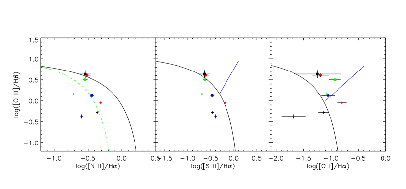
Figure 8: Evolution of TDE targets in BPT diagrams (diamond: SDSS, square: MMT; blue: J0748+4712, red: J0952+2143, green: J1342+0530, black: J1350+2916). Those targets evolve from star-forming region towards extreme star-forming region and weak Seyfert region. The changes are mainly due to the increasing of [O III] and smaller aperture of MMT spectra.

W12 showed that conventional narrow-line ratios measured from the SDSS spectra place these objects in the locus of star forming galaxies on the BPT diagrams (Baldwin, Phillips & Terlervich 1981; also Kewley et al. 2006). This suggests that these lines come mainly from star-forming regions around the nuclei. Figure 8 demonstrates the line ratios measured from the MMT spectra on the BPT diagrams. The line ratios are now very close to or above the line of demarcation between extreme AGNs and the star-formation region. This is at least partially attributed to the increase of [O III] from the nucleus as discussed below.

Changes in the BPT diagram must be interpreted with caution because the SDSS and MMT spectra were obtained using different apertures. The MMT long-slit spectra are extracted from a smaller aperture (1”$\times$3”) than the SDSS fiber size (3” diameter circle), and thus contain less light of the host galaxy. The emission lines from the extended star-formation region should be weaker in MMT spectrum than in SDSS spectrum. Indeed, the low ionization lines, including [S II], [N II], and narrow H$\alpha$, H$\beta$, are substantially weaker in the MMT spectra than in the SDSS spectra(table 2), suggesting that they come from a large region. However, [O III] in the MMT spectra is significantly stronger than in SDSS spectra (Figure 6 and table 2). The difference (360%, 33%,75% and 50% for J0748+4712, J0952+2143, J1342+0530 and J1350+2916) is larger than the calibration uncertainty (typically 4% for SDSS and $<$5% for MMT spectrum). This suggests that [O III]$\lambda$5007 had brightened since the SDSS observation. The increment must come from the very nuclear region that is related to the tidal disruption event.

It is surprising that we measure an [O III] doublet ratio [O III]$\lambda$4959/[O III]$\lambda$5007$\simeq 1/2$, which is very different from the conventional $1/3$, in J0748+4712 and J1342+0530 (Figure 6). To check for potential contamination from other lines, we examined the NIST atomic database for lines within 3Å of [O III]$\lambda$4959. Only Ti I$\lambda$4958.3, Fe II$\lambda$4958.2, Pm I$\lambda$4959.5 and Fe I$\lambda$4961.2 are within 3Å of [O III]$\lambda$4959. Fe II can be ruled out because it would produce much stronger emission at 4889.6Å from the same upper level, which is not detected. For a similar reason, Fe I can be excluded because it predicts a stronger emission line at 4916.3Å. Ti I and Pm I have the same problem in addition to a very small element abundance. Therefore, contamination with other lines can be ruled out. We also looked for potential telluric absorption lines and sky lines around the redshifted line wavelengths and found none. Since [O III]$\lambda$4959 and [O III]$\lambda$5007 share the same upper level, the different line ratios can be only explained by the radiation transfer effect, which requires a substantial optical depth for the line. A detailed interpretation of this is given in §4.2.

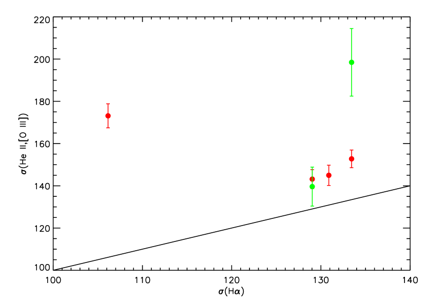
Figure 7: Line width of H$\alpha$ versus the width of [O III] (red) and He II (green) line in four TDE targets in MMT spectra. Only lines with $>$ 3$\sigma$ detection are plotted. The straight line denotes one-to-one relation.

Narrow He II$\lambda$4686 shows a more complicated variability pattern. In J0952+2143, strong narrow He II$\lambda$4686 seen in the SDSS spectrum becomes barely detectable in the MMT spectrum, along with weakening of coronal lines and the broad lines. On the other hand, narrow He II$\lambda$4686 remains unchanged or shows a small increase in J1342+0530 in the course of the decrease of high ionization coronal lines and the appearance of [Fe VII]. The situation is not clear in the other two objects because of either blending with the broad component in the SDSS spectrum or weakness of the line in the MMT spectrum. Note that He II$\lambda$4686 in both SDSS and MMT spectra are systematically broader than other low-ionization narrow emission lines, such as H$\alpha$ and [S II], which mainly come from star forming regions (Figure 7). This is consistent with the expectation that He II$\lambda$4686 is powered mainly by the continuum flare, and star-formation makes little contribution to it.

4 Discussion

4.1 Formation and Evolution of Broad Lines

In our sample, three targets (J0748+4712,J0952+2143,J1350+2916) show broad recombination lines (H$\alpha$, H$\beta$ or He II$\lambda$4686) in the SDSS spectra and all these lines are double-peaked or strongly blue shouldered. Such lines can be formed in biconical outflows launched by the super-Eddington accretion flow, by a fast outflowing unbound stellar debris, or a ring of accreted debris, that are photoionized by strong radiation from the accretion disk. Bogdanović et al. (2004) showed that photoionized debris produces only weak broad H$\alpha$ line ($L({\rm H}\alpha)\sim 10^{37}$ erg s^-1), which is much smaller than the observed one, for the tidal disruption of a solar type star by a black hole of $10^{6}$ M_☉, because the stellar debris is confined within only a small subtending solid angle to the accretion disk. There are several possible way in which emission lines can be enhanced. First, if the star is evolved, e.g., a subgiant, the debris may spread out more in the vertical direction because an evolved star has a much large size, thus producing more reprocessed emission lines. Second, if the star’s orbit mis-aligns with the spin direction of the black hole, the debris disk may receive more light from the accretion disk. Finally, the line equivalent width is likely also dependent on the mass of black hole. Small black holes may produce larger line equivalent widths because the tidal disruption radius is smaller so the stellar debris has a larger covering factor. It remains to be seen whether taking into account all these effects can reproduce the observed line equivalent width. Thus we favor the biconical outflow model because it predicts a large line equivalent width and double-peak profile which are more consistent with observed lines (Strubbe & Quataert 2009).

In either scheme, broad lines are expected to fade on the time scales of months to a year. The fading is caused by both the declining of the ionizing continuum and the evolution of the debris properties or outflows. The variation of the ionizing continuum is qualitatively understood, a nearly constant luminosity at the super-Eddington phase and a power-law decay phase with an index around $-5/3$ to $-5/2$ (Rees 1998; Laodato & King 2009). In either stage, the ionizing continuum becomes softer. In a quasi-steady accretion system, it is expected that the outflow weakens as the accretion rate decreases. Since the accretion rate varies on dynamic time scales, the structure of the outflow is likely complicated. The disk initially launches strong outflows during the super-Eddington phase, which is accelerated to a high velocity. As the accretion rate decreases, the disk will produce a weak outflow, and the radiation acceleration is greatly reduced; after certain time, it may eventually become smaller than the gravitational one, and then outflow decelerates in the gravitational field.

In J0748+4712 and J1350+2916, we can only put upper limits on the lifetime of the broad lines to 5 years. In J0952+2143, we witness the declining of the broad lines. In the NTT spectrum taken 768 days after SDSS spectrum, the redshifted broad Balmer emission lines and double horn profile are still prominent (Komossa et al. 2009). The line flux declined by a factor of only 2.8 in comparison with SDSS observation. This is slower than a $\propto t^{-4/3}$ or $t^{-5/3}$ law if we take the initial flare to have occurred near the SDSS photometric observation, 375 days before the SDSS spectroscopic observation. In its MMT spectrum, which was taken 2187 days after the SDSS spectrum, the double horn profile disappeared but the weak redshifted broad component still exists. Taking into account the short recombination time scale of excited H atoms ($\approx 10^{5}/n_{e}$ yr, Osterbrock & Ferland 2006), an ionizing continuum is needed to produce the broad Balmer lines. The continuum may form through late stage accretion of residuary stellar debris in very eccentric orbits, or by fallback of failed outflows. The broad line flux is a factor of 4 lower than in the NTT spectrum. Noting that both the line width and the centroid offset decreases with time, this is consistent with the decelerating outflow scenario.

Probably due to the relative small size of the accretion disk, outflows from both sides are observed, leaving a double peaked profile, in contrast to the single-peak blueshifted profiles of CIV in luminous quasars (Richards et al. 2011; Wang et al. 2011). The He II line in J0748+4712 is not symmetrical around zero velocity at the source rest frame. This perhaps can be attributed to the partially obscuration of the base of the receding outflow. The small separation between the two peaks in the other two objects can be produced by either a large inclination to the collimated outflows or a small outflow velocity. As noted in W12, J0748+4712 was seen by SDSS much earlier than the other two objects when the disk emission is still strong and outflows show a high velocity. With the decrease of the accretion power, the outflows are decelerated in the gravitational potential of the black hole, leading to small outflow velocities in other two objects.

As discussed in W11 (see also Peterson & Ferland 1986; Gezari et al. 2012), the large He II/H$\alpha$ ratio requires an over-abundance of helium relative to hydrogen, which is interpreted by W11 as the tidal disruption of an evolved star. Following Peterson & Ferland (1986) and assuming a gas temperature of $2\times 10^{4}K$, a minimum of $n_{He}/n_{H}=0.75$ is required by assuming that most of helium is in He⁺².

Most TDEs discovered by X-ray and UV flares do not show broad emission lines, while three of four objects in this sample do. This may be attributed to selection effects. On the one hand, the broad line objects are usually considered as AGN and rejected for further monitoring to reduce the number of sources for repeated spectroscopic follow-up (Gezari et al 2009; van Velzen et al 2011; Cenko et al 2012). On the other hand, coronal-line selected objects preferably lie in the gas-rich disk galaxies, and they tend to host small black holes. The accretion rate is expected to be higher than that of a high- mass black hole, and outflows should be denser and stronger. If broad lines are formed in outflows, one naturally expect that TDE by small black holes produce strong broad emission lines. More theoretical calculations are required to verify this.

4.2 Consequences of optically thick [O III] emission

4.2.1 Simple estimates

The [O III] line ratio, which is $\sim 2$ rather than the expected 3, suggests that the lines are optically thick. In this section we examine some consequences of this observation. This discussion is preliminary because there is not yet sufficient spectroscopic constraints to fully define a model for the observations.

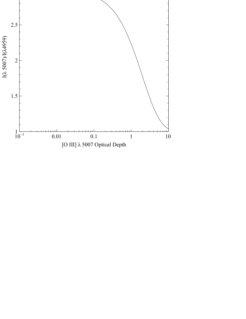
Figure 9: The dependence of the [O III] $\lambda 5007/\lambda 4959$ ratio on optical depth of $\lambda 5007$. A line ratio of $\approx 2$ corresponds to an optical depth $\tau(\lambda 5007)\approx 1.5$.

If a line is thermalized, that is, the density is substantially above the critical density of the line, then the level populations are given by the gas kinetic temperature and line photons are lost in the scattering process because they are collisionally deexcited. The intensity of a line is then given by $I_{\nu}=B_{\nu}[1-\exp(-\tau)]$ where $B_{\nu}$ is the Planck function and $\tau$ the line optical depth. The $\lambda\lambda$5007, 4959 line optical depths $\tau$ are in a 3:1 ratio, so the intensity ratio is given by $I(\lambda 5007)/I(\lambda 4959)=[1-\exp(-\tau)]/[1-\exp(-\tau/3)]\approx 2$. This function is shown in Figure 9. A line ratio of $\approx 2$ corresponds to an optical depth $\tau(\lambda 5007)\approx 1.5$.

The actual line ratio is a function of both optical depth and density. If the electron density is well below the critical density of the ¹D₂ level that produces the [O III] lines then photons will be remitted after absorption. They will simply scatter out of the cloud with no loss of intensity and the 3:1 line ratio is maintained. Line photons are only lost when there is a large probability of collisional deexcitation, they are thermalized, following absorption. The lines will be well thermalized when the density is $n_{e}\gg n_{crit}(^{1}{\rm D}_{2})\approx 6.8\times 10^{5}\ t_{4}^{0.5}\ {\rm cm}^{-3}$, where $t_{4}=T/10^{4}$ K. If the density is less than this, a larger $\lambda 5007$ optical depth would be needed to reach the same line ratio.

More O III lines would be needed to estimate the parameters for the [O III]-forming region. A good detection of the $\lambda 4363$ line would be important. These observations are not available so we will simply assume that the $\lambda 5007$ optical depth is of order unity, $t_{4}=10^{4}$ K, and that the electron density is of order the ¹D₂ critical density.

4.2.2 Column density and Compton depth

The line absorption coefficient is given by

$$\alpha=1.497\times 10^{-6}f_{lu}\lambda_{\micron}/u_{Dop}\ {\rm cm}^{2}$$ (1)

where $f_{lu}$ is the absorption oscillator strength, $\lambda_{\micron}$ the wavelength in microns, and $u_{Dop}$ the Doppler width in velocity units. Assuming the transition probabilities given by Storey & Zeippen(2000) we find $\alpha=5.57\times 10^{-17}u_{Dop}^{-1}\ {\rm cm}^{2}$.

The Doppler width is given by the thermal width if turbulence is absent;

$$u_{th}=\sqrt{2kT/m}\ {\rm cm\ s}^{-1}\approx 12.8\sqrt{t_{4}/m_{AMU}}\ {\rm km\ s}^{-1}\approx 3.2\ t_{4}^{1/2}\ {\rm km\ s}^{-1}$$ (2)

where the expression is evaluated for oxygen, $m_{AMU}=16$. The absorption cross section becomes

$$\alpha=1.74\times 10^{-22}\ t_{4}^{-1/2}\ {\rm cm}^{2}$$ (3)

The column density required for $\tau(\lambda 5007)>1$ is then

$$N({\rm O}^{2+})>5.75\times 10^{21}\ t_{4}^{1/2}\ {\rm cm}^{-2}$$ (4)

The solar O/H ratio is $4.9\times 10^{-4}$ (Asplund et al.2009) so the total hydrogen column density at a metallicity $Z$ will be

$$N({\rm H})>1.2\times 10^{25}\ t_{4}^{1/2}\ Z^{-1}\ {\rm cm}^{-2}$$ (5)

The corresponding electron scattering optical depth is then

$$\tau(e)=\sigma_{T}N({\rm H})>7.8\ t_{4}^{1/2}\ Z^{-1}$$ (6)

where $\sigma_{T}$ is the Thomson cross section. This has the important consequence that, unless the metallicity is quite large ($Z\geq 10$), the [O III] line-forming region is optically thick to electron scattering.

This means that we may have underestimated the line width in Equation 2 since $\lambda 5007$ photons will scatter off the rapidly-moving electrons. The mass of an electron is $2.94\times 10^{4}$ smaller than an oxygen atom so the line width is 171 times wider. The column densities are increased by $\sqrt{171}\simeq 13$ if electron scattering dominates the line width.

The thermal width of [O III] $\lambda 5007$ at $10^{4}$ K would be $\sim 550$ km s^-1 in the electron-scattering dominated limit. This is substantially larger than the observed widths, 200 and 255 km s^-1 , showing that the lines are not broadened into the full electron scattering limit. At optical depth $\tau(e)<1$, the scattered photons will produce an extended wing with a width dependent on the optical depth and electron temperature, supposed on the primary emission profile (Laor 2006). Thus the profile of high velocity wing can be used to constrain the properties of the scatter. Unfortunately, from our data we can not confirm or rule out the existence of the broad wing of [O III] emission lines. The lack of a prominent wing would indicate that the gas has a high metallicity of order $Z\sim 10$.

4.2.3 Suggestions from photoionization models

The large column density suggested in Equation 5 places constraints on the radiation field shape and intensity. In its simplest form the photoionization balance equation may be written as (Osterbrock & Ferland(2006))

$$\phi({\rm H})=n_{e}\,n_{p}\,\alpha_{B}\,dl=n_{e}\,\alpha_{B}\,N({\rm H})$$ (7)

where $\alpha_{B}$ is the hydrogen Case B recombination coefficient, $\phi({\rm H})$ is the flux of hydrogen-ionizing photons, and $dl$ is the Strömgren thickness, the thickness of the H⁺ layer. This can be written in terms of the dimensionless ionization parameter $U$, the ratio of densities of hydrogen-ionizing photons to hydrogen,

$$U({\rm H})\equiv\frac{\phi({\rm H})}{n({\rm H})c}=1.1\,\frac{\alpha_{B}}{c}\,N({\rm H})$$ (8)

where we assume that helium is single ionized with solar metallicity, so that $n_{e}=1.1n({\rm H})$. Putting in numerical values and assuming $\alpha_{B}\approx 2.6\times 10^{-13}\,t_{4}^{-0.8}$, the limit in Equation 5 becomes

$$U({\rm H})>10^{2}\,t_{4}^{-0.3}\,Z^{-1}.$$ (9)

This is a large ionization parameter. Photoionization models of strong-[O III] lined objects are often fitted with $U\sim 10^{-2}-10^{-1}$. For photoionization by a continuum that extends to high energies, such as the SED of an AGN, the ionization of the gas is proportional to $U$ (Osterbrock & Ferland 2006) and little O²⁺ is present for such large values.

This is not the case if the SED is soft. If few ionizing photons are present at energies that can ionize O²⁺ to O³⁺ then the required column density of O²⁺ will be produced. This occurs if the SED is equivalent to a blackbody with $T<5\times 10^{4}$ K, or if a more energetic SED is filtered through in intervening absorbing column which removes high-energy photons. This brings in the nature of the ionizing source, a fundamental question in these objects.

A very large $U$ with a soft SED is consistent with the 10⁴ K temperature we have assumed. In photoionization equilibrium the gas heating is proportional to the photoionziation rate, which is equal to the recombination rate. There is no direct dependence on the flux of photons or the ionization parameter. A stronger flux of photons produces higher ionization but the same photoionization rate, which is equal to the recombination rate, so the heating rate is constant.

4.3 Formation and Evolution of Narrow Emission Lines

Coronal lines and a significant fraction of [O III] must come from ambient gas photoionized by the flare as they are variable on time scales of several years. Most previous TDE candidates that were discovered via X-ray or UV flares do not have such features. The recent discovered TDE candidate PS1−10jh with a strong broad He II$\lambda$4686 line but weak Balmer lines as J0748+4712 do not show coronal lines either (Gezari et al. 2012). Thus only a fraction of TDE shows coronal lines, and the presence of coronal lines can be independent of the existence of broad lines. This can be understood in the framework already discussed. The presence of coronal lines is related to the gas distribution close to the supermassive black hole (W12), while the formation of broad lines depends on the strength of outflows or the geometry of debris relatively to the disk radiation, which is likely anisotropic. Although the nuclear gas environment and outflows are expected to be correlated with the black hole mass in the local universe statistically, there are many outliers.

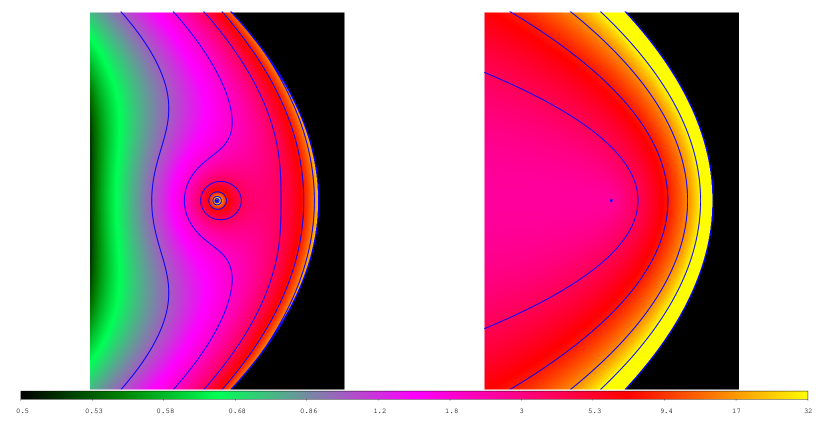
Figure 10: A snapshot of the ionization parameter around a black hole that contributes to the observed emission lines at a specific time in an over-simplified model, in which the ionizing continuum decreases with time as $\propto$ t^-5/3 when t $>$ t₀ (where t₀ is the time between the star was tidal disrupted and most bound material returned to pericenter) and the density distribution decreases as $\propto$ r^-1(left panel) and $\propto$ r^-2(right panel). The observer is to the left of the figure at time 10 t₀. The overlaid blue lines are intensity contours with an interval of two times fold.

Komossa et al. (2008) postulated that coronal lines are echoes of the continuum flare by distant gas. As discussed in W12, the variations of emission lines are rather complex in this scenario, depending on the time evolution of the flare as well as the distribution of gas surrounding the massive black hole. The emission lines at a given time come from different regions that are illuminated by the continuum with different time advances. Thus, in the optically thin case, the optimal emission region for a specific line is determined by competition between the time fading of the continuum, the position dependent time lag, the $r^{-2}$ dilution of incident continuum intensity, and the radial dependence of density. Figure 10 shows the snapshot of ionization parameter distribution for a model in which the ionizing continuum varies with time as a power-law declining phase $L(t)\propto t^{-5/3}$, and a smooth density distribution $n\propto r^{-\beta}$. In the optically thick case, additional frequency dependent attenuation has to be considered, which steepens the ionizing continuum at distant region.

Even with the sparse sampling, the observations clearly require a different duration time scale of coronal lines in different objects. Coronal lines in J1342+0530 lasted for a time scale of at least ten years with a transition from high ionization coronal lines only to low ionization lines only, while in J0748+4712, all coronal lines disappeared in less than 4-5 years. It is not clear what causes the different time scale: the continuum light curve or the gas distribution. We do not know what happened between the SDSS observation in 2004 and Xinglong 2.16m observation in 2009 for J0748+4712. Was there a similar transition from high ionization coronal lines only to low ionization coronal lines, or all coronal lines disappeared simultaneously? Even more, also for J1342+0530 and J1350+2916, is there an intermediate state with both high and low ionization coronal lines as seen J0952+2143? If so, then there is a continuous transition from high to low ionization state and we can unify the high and low ionization coronal line emitter through time evolution. Unfortunately, we do not have the data in these important evolution stages.

[O III] variability provides additional constraints on the gas distribution in the inner parsecs and the evolution of the ionizing continuum. The brightening of [O III] follows the declining of coronal lines, i.e., average ionization of line emitting gas decreases continuously. Giving the short recombination times of O²⁺ ($1.3\times 10^{5}\ (10^{6}\ {\rm cm}^{-3}/n_{e})$ s), the gas is in quasi-ionization equilibrium. This requires either attenuation of the ionizing continuum or/and the density must decrease more slowly than $r^{-2}$. The analysis in the last section suggests a soft ionizing continuum. Combining with the strong coronal line emission in the early spectra, the supports the idea that hard ionizing photons had already been filtered.

We have derived a lower limit on the gas column density in the last section for two sources (J0748+4712 and J1342+0530) with non-canonical [O III] ratios. Bearing in mind that the flare is less than ten years, so $O^{2+}$ ions exist within the region bounded by the parabolic surface with a lag of ten years (see Figure in W12). The large column density sets a lower limit on the gas density of order $n({\rm H})\sim 1.2\times 10^{25}\ t_{4}^{1/2}\ Z^{-1}/c\ \Delta t\ {\rm cm}^{-3}=2\times 10^{6}\ t_{4}^{1/2}\ Z^{-1}\ \Delta t_{6}^{-1}\ {\rm cm}^{-3}$, where $\Delta t_{6}=(\Delta t/6)\ {\rm yr}$.

Assuming that all observed [O III] comes from the same region, we can derive the volume and mass of [O III] emitting gas. At a temperature $10^{4}$ K, the volume emissivities of [O III]$\lambda$5007 are 2.0$\times 10^{-16}$, 1.7$\times 10^{-14}$, 6.7$\times 10^{-13}$ and 9.5$\times 10^{-12}$ erg s^-1 cm^-3 for $n({\rm H})=10^{4}$, $10^{5}$, $10^{6}$ and $10^{7}$ cm^-3 assuming a solar abundance. The observed [O III]$\lambda$5007 luminosities for J0748+4712 and J1342+0530 are similar and around 9$\times 10^{39}$ erg s^-1, requiring a volume of line emitting gas of only 2.7$\times 10^{52}$ cm³ for $n({\rm H})=10^{6}$ cm^-3. This volume is only a small fraction of the volume swept by the flare radiation in nearly 10 years, suggesting a small filling factor. Combining this with a large column density implies that the emission region consists of only a small number of thick clouds.

4.4 Could the Powering Source be AGN Variability?

A substantial fraction of AGNs show coronal lines, but their strengths are usually much weaker than [O III]. In the SDSS spectra, coronal lines of these TDE candidates are 1-2 orders of magnitude stronger than that of strong coronal line emitting Seyfert galaxies. Further, large body of AGN monitoring have shown that coronal lines in most AGNs are quite stable, while in rare cases which coronal lines do vary on time scale of years and the amplification is usually moderate (Penston et al.1984; Veilleux 1988). Only in one extreme case IC 3599, a strong decline of [Fe X] by two orders of magnitudes was observed after an unusual soft X-ray burst by a factor of 100, that was sometimes interpreted as tidal disruption event (Brandt et al. 1995; Grupe et al. 1995; Komossa & Bade 1999). In our four TDE targets, coronal lines with ionization potentials higher than that of [Fe VII] show strong fading of more than two orders of magnitudes within ten years and [Fe VII] lines appear in two targets without them in SDSS spectra. That makes them very extreme if they were AGNs. In addition, large amplitude variations (a factor of 100) in the highly ionized coronal lines require large amplitude variations in soft X-rays. Up to now only narrow line Seyfert 1 galaxies and BL Lac objects are known to show such large amplitude variability in X-rays (Eracleous et al.2012). All the seven ECLEs targets are covered by FIRST survey (Becker et al. 1995), but only J0938+1353 was detected with a low flux of 1.93 mJy, while others are below the detection limit, typical 1 mJy. So from optical spectrum and radio flux, we can rule out both possibilities.

Along with the variation of coronal lines, a significant increase of [O III] emission lines is detected in the four TDE targets. There is no clear evidence that emission lines such as [O III] from normal AGN NLR would show strong variability due to its large size. So persistent AGN activity is very unlikely the powering source of the variation of coronal lines and [O III] lines.

The disappearance of broad emission lines are also very different from other Seyfert galaxies monitoring so far. In these Seyfert galaxies, broad emission lines usually vary in response to changes in the continuum with a moderate amplitude. Only two cases were reported for temporary disappearance of broad emission lines over a period of a few months accompanying with large continuum variations in NGC 4151 and NGC 5548 (Penston & Perez, 1984; Iijima et al. 1992). In J0748+4712 and J0952+2143, which have several observations after the outburst, we only find broad lines are either fading or disappeared. Therefore, there is no evidence for re-starting of the central engine. Considering all these facts, we believe that the powering source is likely a strong outburst in an quiescent galaxy rather than stochastic variability of an AGN.

4.5 Could the Powering Source be Supernova Explosion?

For the Supernova (SN) scenario, it is unable to explain the high luminosities of coronal lines and the absence of other low-ionization lines, and the continuum variability in some targets(W12). Also, the MMT follow-up observations provide additional constraints on the SN scenario. First, four TDE candidates show an increase of [O III] between SDSS to MMT observations, and the [O III] are systematically broader than normal low-ionization lines such as H$\alpha$ (figure 7). This characteristic is different from other known SN. Very few young SNs display variable narrow [O III] emission. Some SNs do show [O III] emission a few years to up 100 years after explosion, but these lines are usually broad, accompanying low ionization lines of similar widths (Milisavljevic et al. 2012). They are formed in the SN shell interacting with the stellar winds. Second, based on the total energy in the high ionization coronal lines, W12 estimated a total energy in soft X-ray of order $10^{50}$ ergs. The emergence of [Fe VII] lines in these two objects with only high ionization coronal lines in previous SDSS spectra (J1342+0530 & J1350+2916) and the persistence of [Fe VII] in J0952+2143 suggest that a strong UVX ionizing continuum is still seen by the line emitting gas. The brightening of the He II$\lambda$4686 line in J1342+0530 indicates a further increase of EUV ionizing photons absorbed by line emission gas in this object, probably arising from large covering factor of gas at the time lag. These variations of [Fe VII] and He II$\lambda$4686 lines re-enforce the conclusion in W12 that a very energetic flare is required to power the coronal line emission.

As shown in the last section, the presence of an optically thick [O III] emission region requires large ionization parameters. In echo models, gas is photoionized by the continuum flare that took place 5-9 years ago, so the size of emission line region is $R_{\rm[OIII]}\simeq 1-3$ pc. The peak luminosity of ionizing continuum can then be estimated from the ionization parameter, the distance and the density,

$$L_{ion}=4\pi R_{\rm[O\sc III]}^{2}n({\rm H})U({\rm H})c\langle h\nu\rangle>7.9\times 10^{45}t_{4}^{-0.3}Z^{-1}R_{pc}n_{6}({\rm H})\ {\rm erg\ s}^{-1}$$ (10)

with a reasonable $n_{6}({\rm H})=n({\rm H})/10^{6}{\rm cm}^{-3}\sim 1$, the luminosity would be $10^{45-46}$ erg s^-1, which is much more luminous than any supernova and is close to the Eddington limit for a $10^{7-8}$ M_☉ black hole. Finally, the life time of broad lines are at most several years, which is much shorter than these in type II SN.

5 Conclusions

We have carried out follow-up MMT observations of seven extreme coronal line emitters that were studied by W12. Three objects turn out to be persistently strong coronal line emitters. Among them, two are likely star-forming and AGN composite or tidal disruption of a giant star, and one is a narrow line Seyfert 1 galaxy. In the other four objects, all coronal lines with ionization higher than [Fe VII] disappear. Thus, they are tidal disruption candidates. [Fe VII] lines faded in J0952+2143 and appear in the MMT spectra of two objects with higher ionization coronal line only in SDSS spectra. [O III] doublets are brightened in all four objects. Thus we are still witnessing echoes of the continuous decrease of the gas ionization in the emitting region. If this trend continues, the object will appear in the AGN locus of the BPT diagram. Further monitoring of the emission lines is needed.

We also detected non-canonical [O III] ratios in two objects. The column density of $O^{2+}$ must be large to make [O III]5007 optically thick. For reasonable metallicity, the H column density is large and the gas is probably optically thick to electron scattering. Lines will be broadened due to electron scattering, which can be tested with future high quality data. The ionization parameter has to be very large to get this column density, and this also requires that the ionizing SED be relatively soft, equivalent to a $T<5\times 10^{4}$ K blackbody, or oxygen would be too ionized. A gas temperature of order 10⁴ K will occur for such extreme conditions due to the nature of photoionization equilibrium, if the SED is this soft.

These observations can be fitted into a picture where giant molecular clouds are illuminated by continuum flares with an ionizing continuum luminosity of order $10^{45-46}$ erg s^-1 within a few parsecs of the nucleus. The gas in the inner face of the cloud produces the coronal lines. As high energy photons are absorbed by the gas, the ionizing continuum illuminating outer part of the clouds softens and creates a thick [O III] emission region. The presence of giant molecular clouds in the center parsec and no persistent nuclear activity is striking, suggesting that perturbation in the gas is more fundamental for the black hole fueling. Clearly, we still miss some critical evolution phases, which prevents us from probing a direct connection between these two subclasses of extreme coronal line emitters. Future follow-ups of new discoveries of such objects from the spectroscopic surveys of LAMOST and BigBOSS can fill the gaps and yield a more complete picture of emission line evolution.

Broad emission lines previously seen in the SDSS spectra of J0748+4712 and J1342+0530 vanished in the MMT spectra, and there is only weak broad Balmer lines in J0952+2143. In J0952+2143, we observed continuously fading of the broad lines by a factor of 11 in past 8 years as well as a decrease of the line width and velocity shift. The line profile variability perhaps reflects the deceleration of emission line gas in the gravitational field of the black hole due to a lack of further radiative acceleration. With improved subtraction of stellar light, the broad lines in these objects are found to all be double-peaked or blue-shouldered, suggesting it is a general property, probably from biconical outflows.

Table 1: Basic Data of Extreme Coronal Line Emitters

No	Name	$z$	$M_{i,{\rm tot}}$	Obs Interval	Broad Line	[Fe VII]		[O III]	NSC
						SDSS	MMT		SDSS	MMT
1	SDSS J074820.66+471214.6	0.0615	-19.75	2866	fading	no	no	increase	yes	no
2	SDSS J095209.56+214313.3	0.0789	-20.41	2187	fading	yes	yes	increase	no	no
3	SDSS J134244.42+053056.1	0.0366	-18.91	3548	absence	no	yes	increase	no	no
4	SDSS J135001.49+291609.7	0.0777	-19.76	2073	fading	no	yes	increase	no	no
5	SDSS J093801.64+135317.0	0.1006	-21.29	1834
6	SDSS J105526.43+563713.3	0.0743	-20.01	3548
7	SDSS J124134.26+442639.2	0.0419	-19.95	2859

Table 2: Narrow Emission Line Flux of Variable Targets

No	H$\alpha$	H$\beta$	H$\alpha$	H$\beta$	[Ne III]	[He II]	[N II]	[O I]	[O III]	[O III]	[O III]	[Fe VII]	[Fe VII]	[S II]	[S II]
					$\lambda$3896	$\lambda$4686	$\lambda$6583	$\lambda$6300	$\lambda$4363	$\lambda$4959	$\lambda$5007	$\lambda$5722	$\lambda$6088	$\lambda$6716	$\lambda$6731
1	$131(4)$	$49(4)$			$<2$	$<6$	$48(4)$	$12(3)$	$<8$	$31(4)$	$65(4)$	$<3$	$<4$	$23(4)$	$21(4)$
2	$108(7)$	$26(4)$	$155(10)$	$39(7)$	$31(4)$	$11(3)$	$64(5)$	$14(4)$	$<16$	$72(3)$	$215(3)$	$13(3)$	$17(5)$	$25(4)$	$27(4)$
3	$171(5)$	$27(4)$				$33(4)$	$49(4)$	$20(5)$	$<15$	$92(3)$	$182(3)$	$18(3)$	$31(4)$	$23(5)$	$17(5)$
4	$79(5)$	$15(3)$				$6(2)$	$22(4)$	$<5$	$<9$	$22(1)$	$66(1)$	$8(2)$	$12(4)$	$9(2)$	$9(2)$

Figure 6: [O III] lines of four TDE targets. Same order and color as figure 5.

References

- (1) Asplund, M., Grevesse, N., Sauval, A. J., & Scott, P. 2009, ARA&A, 47, 481
- (2) Ayal, S., Livio, M., & Piran, T. 2000, ApJ, 545, 772
- (3) Baldwin, J. A., Phillips, M. M., & Terlevich, R. 1981, PASP, 93, 5
- (4) Becker, R. H., White, R. L., & Helfand, D. J. 1995, ApJ, 450, 559
- (5) Bogdanović, T., Eracleous, M., Mahadevan, S., Sigurdsson, S., & Laguna, P. 2004, ApJ, 610, 707
- (6) Brandt, W. N., Pounds, K. A., & Fink, H. 1995, MNRAS, 273, L47
- (7) Bruzual, G., & Charlot, S. 2003, MNRAS, 344, 1000
- (8) Cenko, S. B., Bloom, J. S., Kulkarni, S. R., et al. 2012, MNRAS, 420, 2684
- (9) Esquej, P., Saxton, R. D., Komossa, S., et al. 2008, A&A, 489, 543
- (10) Ferrarese, L., & Merritt, D. 2000, ApJ, 539, L9
- (11) Gebhardt, K., Bender, R., Bower, G., et al. 2000, ApJ, 539, L13
- (12) Gezari, S., Halpern, J. P., Komossa, S., Grupe, D., & Leighly, K. M. 2003, ApJ, 592, 42
- (13) Grupe, D., Beuermann, K., Mannheim, K., et al. 1995, A&A, 299, L5
- (14) Gezari, S., Basa, S., Martin, D. C., et al. 2008, ApJ, 676, 944
- (15) Gezari, S., Heckman, T., Cenko, S. B., et al. 2009, ApJ, 698, 1367
- (16) Gezari, S., Chornock, R., Rest, A., et al. 2012, Nature, 485, 217
- (17) Hills, J. G. 1975, Nature, 254, 295
- (18) Kewley, L. J., Groves, B., Kauffmann, G., & Heckman, T. 2006, MNRAS, 372, 961
- (19) Komossa, S., & Bade, N. 1999, A&A, 343, 775
- (20) Komossa, S., Zhou, H., Wang, T., et al. 2008, ApJ, 678, L13
- (21) Komossa, S., Zhou, H., Rau, A., et al. 2009, ApJ, 701, 105
- (22) Kormendy, J., & Richstone, D. 1995, ARA&A, 33, 581
- (23) Laor, A. 2006, ApJ, 643, 112
- (24) Iijima, T., Rafanelli, P., & Bianchini, A. 1992, A&A, 265, L25
- (25) Lodato, G., King, A. R., & Pringle, J. E. 2009, MNRAS, 392, 332
- (26) Lu, H., Zhou, H., Wang, J., et al. 2006, AJ, 131, 790
- (27) Magorrian, J., Tremaine, S., Richstone, D., et al. 1998, AJ, 115, 2285
- (28) Milosavljević, M., Merritt, D., & Ho, L. C. 2006, ApJ, 652, 120
- (29) Milisavljevic, D., Fesen, R. A., Chevalier, R. A., et al. 2012, ApJ, 751, 25
- (30) Oliva, E. 1997, IAU Colloq. 159: Emission Lines in Active Galaxies: New Methods and Techniques, 113, 288
- (31) Osterbrock, D. E., & Ferland, G. J. 2006, Astrophysics of gaseous nebulae and active galactic nuclei, 2nd. ed. by D.E. Osterbrock and G.J. Ferland. Sausalito, CA: University Science Books, 2006
- (32) Penston, M. V., & Perez, E. 1984, MNRAS, 211, 33P
- (33) Penston, M. V., Fosbury, R. A. E., Boksenberg, A., Ward, M. J., & Wilson, A. S. 1984, MNRAS, 208, 347
- (34) Peterson, B. M., & Ferland, G. J. 1986, Nature, 324, 345
- (35) Rees, M. J. 1988, Nature, 333, 523
- (36) Richards, G. T., Kruczek, N. E., Gallagher, S. C., et al. 2011, AJ, 141, 167
- (37) Storey, P. J., & Zeippen, C. J. 2000, MNRAS, 312, 813
- (38) Strubbe, L. E., & Quataert, E. 2009, MNRAS, 400, 2070
- (39) Ulmer, A. 1999, ApJ, 514, 180
- (40) van Velzen, S., Farrar, G. R., Gezari, S., et al. 2011, ApJ, 741, 73
- (41) Veilleux, S. 1988, AJ, 95, 1695
- (42) Wang, H., Wang, T., Zhou, H., et al. 2011, ApJ, 738, 85
- (43) Wang, T.-G., Zhou, H.-Y., Wang, L.-F., Lu, H.-L., & Xu, D. 2011, ApJ, 740, 85
- (44) Wang, T.-G., Zhou, H.-Y., Komossa, S., et al. 2012, ApJ, 749, 115