Optimizing the Determination of
the Neutrino Mixing Angle $\theta_{13}$ from Reactor Data

Abstract

The technical breakthroughs of multiple detectors developed by Daya Bay and RENO collaborations have gotten great attention. Yet the optimal determination of neutrino mixing parameters from reactor data depends on the statistical method and demands equal attention. We find that a straightforward method using a minimal parameters will generally outperform a multi-parameter method by delivering more reliable values with sharper resolution. We review standard confidence levels and statistical penalties for models using extra parameters, and apply those rules to our analysis. We find that the methods used in recent work of the Daya Bay and RENO collaborations have several undesirable properties. The existing work also uses non-standard measures of significance which we are unable to explain. A central element of the current methods consists of variationally fitting many more parameters than data points. As a result the experimental resolution of $\sin^{2}(2\theta_{13})$ is degraded. The results also become extremely sensitive to certain model parameters that can be adjusted arbitrarily. The number of parameters to include in evaluating significance is an important issue that has generally been overlooked. The measures of significance applied previously would be consistent if and only if all parameters but one were considered to have no physical relevance for the experiment’s hypothesis test. Simpler, more transparent methods can improve the determination of the mixing angle $\theta_{13}$ from reactor data, and exploit the advantages from superb hardware technique of the experiments. We anticipate that future experimental analysis will fully exploit those advantages.

I A Technological Breakthrough

It goes without saying that experiments with great technical accomplishment should be evaluated with data analysis of equal or better quality. During the past year or so, the achievement of constructing multiple, nearly identical neutrino detectors by the Daya Bay db1 ; db2 and RENO reno collaborations has been rightly praised as a technological breakthrough. Beyond increasing data rates, the prime function of the new technology is to reduce systematic errors. Systematic errors previously dominated neutrino oscillation experiments with nuclear reactor sources for many years. Yet by a curious gap in the current literature, the data analysis published to quantify the neutrino mixing angle pont ; mns $\theta_{13}$ is far from optimal. Applying more effective methods to the analysis can yield higher resolution of neutrino physics parameters than currently available. Despite lacking complete access to the full information, we can make a case for producing better determination of $\sin^{2}(2\theta_{13})$ and its uncertainties than the experimental reports. We are naturally surprised by this fact. It is primarily due to unrecognized faults in the inefficient methods used before.

The experimental uncertainties on $\theta_{13}$ have been the center of attention for years after the CHOOZ null results of 1999 and 2003 chooz . Uncertainties remained the focus after the upgraded Double Chooz dchooz1 report of new results just before Daya Bay’s and RENO’s results, their improved, 2.9$\sigma$ result a few months later dchooz2 , and a recent result consistent with all previous measurements, but using the delayed neutron capture from hydrogen for the first time dchooz3 . What has gone largely unnoticed is that the statistical method used in these papers diverged significantly from most previous work, cannot directly be compared, and shows signals of being problematic.

There usually exists more than one “correct forms” of data analysis. Most physicists agree one should not be overly concerned with any method, provided the assumptions are reported, that the method is robust under small perturbations, and that the results are reproducible. We will present such a method analyzing the Daya Bay data. The method includes stating a specific hypothesis, which may appear quaint, but if neglected leads to no hypothesis to test. The method uses few rather than many parameters, and we report everything needed to reproduce our calculations. Remarkably, the current experimental literature on $\theta_{13}$ is not definite on any hypothesis, is not reproducible, and its approach does not appear robust under small model parameters that can be freely adjusted.

Once the ground rules are defined, quantifying confidence levels with goodness of fit statistics becomes meaningful. Without ground rules and reproducibility the dependence of a statistic on a parameter has little objective meaning. The tendency to name all statistics “$\chi^{2}$” regardless of their actual definition does not make them all equivalent. When the meaning and values of parameters are omitted from discussion, it is impossible to know whether or not they are “nuisance parameters.” A textbook nuisance parameter is one whose value is completely irrelevant to the hypothesis, but which must be accounted for in the analysis of the parameters that are relevant. Meanwhile there are few if any textbook nuisance parameters in experimental physics. Every parameter has a physical meaning. If a data fit finds a parameter far from expectations, it indicates something is wrong, whether or not the nuisance is annoying. Such a nuisance parameter can invalidate the entire study, depending on its value. Unless one finds a reason otherwise, it is unavoidable that both the “uninteresting” and the “interesting” parameters contribute to the actual hypothesis and its uncertainties.

The upshot is that using extra parameters will carry a statistical penalty if one cares about them. Extra parameters should not be used if one does not care about them. Having it both ways is a impossible for us to defend. After the first version of this paper amirv1 , we undertook a literature search to review the history. It turns out that the references of the Daya Bay experimental proposal DBproposal actually employed a more conservative determination of confidence regions, consistent with ours and contradicting the method Daya Bay used when the data appeared. This is discussed further in Section II.0.2.

Section II begins with a simple straightforward procedure with a clearly stated hypothesis including a list of parameters central to the hypothesis. We will discover an opportunity to retrospectively re-classify a parameter as a nuisance after it was fit and found consistent with expectations. Since that step would abolish the original test conditions, we cannot find a way to justify it. The hypothetical case that our fit stands on a better footing than Daya Bay’ hinges on the fact we account for all our parameters and pay the statistical penalty up front: plus our calculations are reproducible. Section III sets up an illustration of the method of $\chi^{2}$ with pull fogli1 ; sksolar ; strumia ; degouvea ; huber03 that has become the exclusive tool of analysis by the experimental collaborations cited. The method uses many parameters of physical importance, and also turns out to be remarkably sensitive to fine details of tuning external parameters. We explore the method while stating our assumptions, sticking to them, and also provide all the information to reproduce our calculations. This fills a gap in the neutrino literature where the procedures of assigning errors have not been spelled out for the users of the data. When we compare our results following standard procedures with the number of data points and (very large) number of parameters used by Daya Bay and RENO there is a unexplained discrepancy. We cannot explain what hypothesis those experimental groups are assuming, nor find it stated anywhere. The Section also explains how, paradoxically, a definite insensitivity of $\chi^{2}$ defined in that approach is not the virtue it appears. Excessive parameters tends to degrade the determination of the physical objective, $\sin^{2}(2\theta_{13})$. Due to this situation, there is enough leeway in the current determination of $\theta_{13}$ to make two logical but contradictory arguments. It is possible to find the uncertainty of $\theta_{13}$ has been greatly underestimated, and it is also possible to find the uncertainty has been significantly overestimated. Though we are obviously not in a position to resolve the alternatives, we find it fascinating to understand the issues and develop means to assess the situation. That leads to our main conclusion (Section IV) that simpler methods are preferred, both for scientific and mathematical reasons. An Appendix gives details on how we extracted data from the publications.

II Errors Depend on the Procedure

II.0.1 A Straightforward, Simple Approach

For our first example we present a straightforward, simple model. We use the Daya Bay ($DB$) data of Ref. db1 to illustrate the concepts.

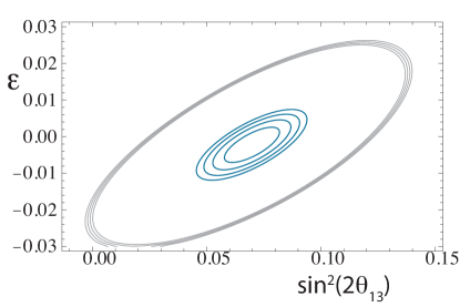
Figure 1: Contours of constant $\chi^{2}$ of the simple 2-parameter fit, Eq. 1. Inner contours (blue online) are the minimum value of 5.66 plus 1, 2, 3, 4 units. Outer contours are also separated by 1 unit and begin at $\Delta\chi^{2}=37.6$ units, the value for the null hypothesis $sin^{2}(2\theta_{13})=0$. The significance of $\Delta\chi^{2}=32$ evaluated using a 2-parameter fit is the equivalent of 5.4 $\sigma$.

The object of the exercise is to determine $\sin^{2}(2\theta_{13})=s_{213}^{2}$ using a model $M_{d\,Model}$ for the $d$th detector. The model assumes a certain reactor flux and detector efficiency, which have a parameter $\epsilon$ describing its relative uncertainty. We cannot avoid $\epsilon$ and need to determine it self-consistently. Our null hypothesis is that $\epsilon$ is of order $1\%\pm 1\%$, and that $s_{213}^{2}=0.$ The point of fitting the data will be to find whether the null model can be ruled out, and compute confidence levels on the two parameters fit relative to the null model used.

Let $M_{d}$ be the total number of events seen in the $d$-th detector. We define a statistic

$$\chi^{2} =\sum_{d=1}^{dmax}\frac{(M_{d}-M_{d\,Model})^{2}}{M_{d}};$$

$$M_{d\,Model} =(1-s_{213}^{2}s_{d}^{2})M_{d\,0}(1+\epsilon)$$

$$=P_{d}M_{d\,0}(1+\epsilon).$$ (1)

Here $M_{d0}$ is the number of events expected with no oscillation, $s_{d}^{2}=<\sin^{2}(\Delta m_{13}^{2}L_{d}/E_{\nu})>$ is averaged over the energy flux at flux-weighted reactor-detector separation $L_{d}$. The denominator $(\sqrt{M_{d}})^{2}$ is the conventional variance from Poisson statistics.

Consider a one-detector experiment like Double Chooz dchooz1 ; dchooz2 . Then $(1-s_{213}^{2}s_{1}^{2})M_{1\,0}(1+\epsilon)$ in Eq. 1 is a single number that cannot determine two variables $s_{213}^{2}$ and $\epsilon$. Due to that degeneracy the ignorance in reactor flux and detector response directly translates into systematic error in $s_{213}^{2}$, and neither can be determined unambiguously.

Consider an experiment like RENO reno with $2$ detectors at $2$ well-chosen baselines. With 2 data points the degeneracy is removed, but parameters are just barely determined, not over-determined. To a good approximation Daya Bay also has 2 flux-weighted baselines, as one can see from their Figure 4, reproduced here as Fig. 2. There is a near set at $(0.467,0.474,0.578)$ km and a far set at$1.647$ km (the separations of the far set are for visualization). The existence of $3$ near and $3$ far detectors effectively triples the amount of data. Due to this situation we do not anticipate a fit to two parameters will be over-determined.

$Detector$	1	2	3	4	5	6
$M_{d0}$	28647	29096	22335	3567	3573	3536
$P_{d}$	0.991	0.977	0.987	0.941	0.929	0.913
$M_{d}$	28389	28427	22045	3356.5	3319	3228
$L_{eff\,d}$	0.474	0.467	0.578	1.647	1.647	1.647

Table 1: Data used in fits. Units of $L_{eff\,d}$ are km.

We fit the simple model with the data shown in Table I, derived in the Appendix. The fit gives $\chi^{2}=5.66$ at $\epsilon=-0.002,\,s_{213}^{2}=0.070\pm 0.018$. A difference of nearly $32$ units of $\chi^{2}$ separate $\chi^{2}(s_{213}^{2}=0),\epsilon=0.01$ from the best fit value. We emphasize that both $\epsilon$ and $s_{213}^{2}$ are meaningful, so that the standard evaluation of significance of “detection” uses $\chi_{2}^{2}$. We review the reasoning behind this next.

II.0.2 Defining Measures of Significance

When data fitting a model comes from a Gaussian distribution, or more generally any distribution with a suitably isolated “bump,” then the statistic $z=\chi^{2}$ is predicted to be distributed by the $\chi_{\nu}(z)$ distribution:

$$\chi_{\nu}(z)=\frac{2^{-\nu/2}}{\Gamma(\nu/2)}e^{-z/2}z^{\frac{\nu}{2}-1}.$$

The estimated number of degrees of freedom $\nu=N-p$ when there are $N$ terms in $\chi^{2}$ and $p$ parameters. We have $N=6$ and $p=2$ hence $\nu=4$, as far as the best-fit is concerned. But rather than focusing on value of $\chi^{2}$, we are concerned with the difference $\Delta\chi^{2}$ between the values of two hypotheses. When two models are nested, meaning one is smoothly immersed in the other by varying $q$ parameters, Wilks’ Theorem predicts $\Delta\chi^{2}$ is distributed by $\chi_{q}^{2}$. The theorem is more general than assuming a Gaussian distribution, but that is not our point. For now, we are emphasizing the decision to use $\nu=2$ for the specific 2-parameter question of “detection.” It is supported by a theorem, and we confirmed it by simulations, yet assessment with $\nu=2$ is a decision based on definite assumptions that we have listed.

The outcome then rejects the null hypothesis $s_{213}^{2}=0$ by the Gaussian equivalent of 5.4$\sigma$. The result is quite close to the significance of 5.2$\sigma$ reported by $DB$ for the same data set. However we will soon see this is a coincidence because $DB$’s criteria of significance are much different from those we illustrate here.

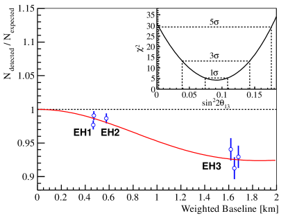
Figure 2: Daya Bay’s Figure 4, showing the survival probability at best fit. The 1$\sigma$, 3$\sigma$, and 5 $\sigma$ confidence intervals of the inset indicate significance is evaluated using the standard one-parameter criterion $\chi_{1}^{2}$. Digitizing the red curve gives the energy and efficiency-averaged detector response.

Parameter uncertainties are quite a different thing from testing hypotheses. In Section I we mentioned the practice of citing parameter uncertainties using $\Delta\chi^{2}=1$. When a fit uses only one (1) parameter the 68% confidence interval coming from $\chi_{1}^{2}$ (note subscript “1’)’ is indeed the range where $\Delta\chi^{2}=1$. Our simple fit uses 2 parameters which jointly need to be monitored. Then it is standard practice pdgstats ; recipes to evaluate significance of the two-dimensional parameter region using the $\chi_{2}^{2}$ distribution. (Note subscript “2”). This statistical penalty takes into account the extra freedom for either parameter to “float” while the other is varied. The error ellipse from two parameters requires $\Delta\chi_{2}^{2}=(2.3,\,6.17,\,11.8)$ to generate $(1\sigma,\,2\sigma,\,3\sigma$) confidence levels. Following standard practice we effectively used the contours of $\chi^{2}=\chi_{min}^{2}+2.3=7.95$ in reporting the uncertainty in $s_{213}^{2}=0.070\pm 0.018$, which can be checked with Figure 1. Notice that this contour crosses close to the prior value of $\epsilon\sim 0.01$. The self-consistency of $\epsilon$ gives confidence that the value of $\,\,\,s_{213}^{2}$ is reliable.

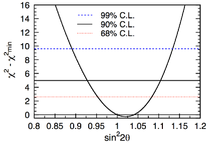
Figure 3: A panel from Figure 39 of Ashie et al ashie showing confidence levels used for a 2-parameter fit. Compare the 1$\sigma$ (68%) and 3$\sigma$ (99.5%) levels of the inset of Figure 2.

Our reason for dwelling on $\epsilon$ does not come from intimate knowledge of the hardware. We care about $\epsilon$ because if the central value fit had been 0.03, for example, we’d distrust the value of $s_{213}$ and its error bars. In no way could we call $\epsilon$ a nuisance parameter. Support for our procedure comes from Fukuda et al. fukuda and Ashie et al. ashie , which are concerned with jointly fitting $\nu_{\mu}\rightarrow\nu_{\tau}$ oscillations with two parameters $\Delta m^{2}$ and $\sin^{2}(2\theta)$ . Both papers make an explicit statement that the 2-parameter procedure uses different criteria than a 1-parameter procedure. Both papers were cited for the statistical method by the Daya Bay experimental proposal. These papers cite $\Delta\chi^{2}=$ 2.6, 4.6, 9.6 for 68%, (1$\sigma$) 90% and 99% ($\sim 3\,\sigma$) confidence regions . Figure 3 is taken from Figure 39 of Ref. ashie and shows how the $n=\sigma$ lines differ from the inset of Figure 2.

Given that $\epsilon=-0.002$ is very small, we might have retrospectively set it to zero, and re-fit the data to one parameter. That sounds like cheating. However if one had been highly confident that $\epsilon=0$, or any other number with negligible uncertainty, it is legitimate to state that information as a definite hypothesis. Under that new hypothesis a one-parameter fit is made with $\epsilon$ fixed and varying $s_{123}^{2}$. The value of having high quality advance information and a one-parameter hypothesis is that $\Delta\chi^{2}$ is distributed by $\chi_{1}^{2}$. Using $\chi_{1}^{2}$ for assessment only needs $\Delta\chi^{2}=1,\,4,\,9...$ for the equivalent $1\sigma,\,2\sigma,\,3\sigma...$ confidence regions. When using $\chi_{1}^{2}$ the significance of $\Delta\chi^{2}=32$ gets upgraded from a 5.4$\sigma$ to a 5.65$\sigma$ determination. More importantly, the reported errors on $s_{213}^{2}$ are reduced from the 2-parameter $\Delta s_{213}^{2}=\pm 0.018$ to $\Delta s_{213}^{2}=0.007$. The new errors, which are less than half the previous ones, are equivalent to finding $\Delta s_{213}^{2}=1$ along the line $\epsilon=0$ intersecting the $\Delta\chi^{2}=1$ contour of Figure 1.

While it is possible to argue further, we do not find a one-parameter fit convincing and we will not choose to ignore $\epsilon$ to reduce our error bars. It is not a question of setting $\Delta\chi^{2}=1$, or plotting $\Delta\chi^{2}$ as a function of $s_{213}$. The issue is to make the definition of the confidence region and the test being conducted consistent. By starting with a hypothesis that extreme values of $\epsilon$ can invalidate the analysis we are committed to accounting for it as a central parameter.

II.0.3 Connection with the Daya Bay Analysis

This is the first point where we notice an uncommon standard has entered the neutrino literature. First, the texts of the $DB$ papers db1 ; db2 do not specifically spell out the basis of their confidence level assignments. No hypothesis is stated, yet two parameters of an absolute normalization $\epsilon$ and $\sin^{2}(2\theta_{13})$ are cited in their same paragraph. How is $\Delta\chi^{2}$ being evaluated?

Figure 4 of Ref. db1 , reproduced as Fig. 2, allows one to deduce the method. The inset of the figure shows the $1\sigma,\,3\sigma,\,5\sigma$ variations occurring at $\Delta\chi^{2}=1,\,9,\,25$. This established significance is being evaluated via $\chi_{\nu}^{2}$ with the number $\nu=1$.

If one were comparing the hypothesis of $s_{213}^{2}\neq 0$ (best fit) with $s_{213}^{2}=0$ (null) we would agree. The hypothesis of $s_{213}^{2}=0$ has been ruled out. What is uncommon is to evaluate the uncertainty or “standard error” of $s_{213}^{2}$ also using $\chi_{\nu}^{2}$ with the number $\nu=1$. There are 19 other background parameters floating to their best fit values, developing a 20-dimensional error ellipsoid, while errors have been found with no statistical penalties and using $\chi_{\nu}^{2}$ with the number $\nu=1$. Are all 19 parameters irrelevant nuisance parameters, whose value has no bearing on the experiment?

$DB$ seems to suggests a penalty of a 2-parameter fit in citing $\chi_{Daya\,Bay}^{2}/NF=4.6/4$, where $NF$ is the number of degrees of freedom, and two parameters in the text. Besides citing $\sin^{2}(2\theta_{13})$ they write “the absolute normalization $\varepsilon$ was determined from the fit to the data.” One might interpret $NF=4$ to mean 6 data points minus 2 ”important” parameters ($\epsilon$ and $\sin^{2}(2\theta_{13})$). Actually there are 24 terms in $\chi_{Daya\,Bay}^{2}$, which is fit with 20 parameters to give $NF=24-20=4$. The formula is:

$$\chi_{Daya\,Bay}^{2} = \sum_{d=1}^{6}\frac{\left[M_{d}-T_{d}\left(1+\varepsilon+\sum_{r}^{6}\,\omega_{r}^{d}\alpha_{r}+\varepsilon_{d}\right)+\eta_{d}\right]^{2}}{M_{d}+B_{d}}$$

$$+\sum_{r}^{6}\,\frac{\alpha_{r}^{2}}{\sigma_{r}^{2}}+\sum_{d=1}^{6}\left(\frac{\varepsilon_{d}^{2}}{\sigma_{d}^{2}}+\frac{\eta_{d}^{2}}{\sigma_{Bd}^{2}}\right).$$ (2)

Symbol $T_{d}$ is the prediction from neutrino flux, $MC$ (simulations), and neutrino oscillations, which involves integrating over the reactor energy spectrum, and detector mass and acceptance, using a model.

The formula has 18 variationally-determined “pull parameters” in the set $\alpha_{r},\,\varepsilon_{d}$, and $\eta_{d}$. The set of 20 parameters is completed with $\varepsilon$ and $\sin^{2}(2\theta_{13})$. Constants given are $\sigma_{r}=0.8\%$, the uncorrelated reactor uncertainty, $\sigma_{d}=0.2\%$ the uncorrelated detection uncertainty. Symbol $B_{d}$ is the background corresponding to data set $M_{d}$, and $\sigma_{Bd}$ the background uncertainties of a few percent of the total number of events. We added subscript $d$; the paper states that the values are given in a Table, which unfortunately is not complete. The fraction of inverse beta decays from the $r$-th reactor to the $d$-th detector as determined by baselines and reactor fluxes is denoted $\omega_{r}^{d}$, a $6\times 6$ array not available from the paper or elsewhere.

Just as in our simple model fit, $DB$’s decision to use $\nu=1$ to assess a 20-parameter fit makes a difference in the definition of the confidence level. The choice of $\nu=1$ has not been explained. Our analysis appears to be the first to notice this decision might be questioned. For example, if nobody cared about the value of $\epsilon$, $\alpha_{r},\,\varepsilon_{d}$, and $\eta_{d}$, and nobody looked to find them reasonable, we’d be very surprised, yet agree with $\chi_{1}^{2}$ confidence levels, because we don’t have the authority to disagree. But for every parameter whose fit value could have possibly invalidated the analysis, there is usually a statistical penalty for introducing it, and reporting of fit values once they are found. $DB$ evidently did examine 20 parameters with serious concern for their values, writing db1 that ”All best estimates of pull parameters are within its (sic) 1 standard deviation based on corresponding systematic uncertainties”.

III The method of $\chi^{2}$ with pull

The method of $\chi^{2}$ minimization with pull parameters ($\chi^{2}-pull$) was introduced for neutrino oscillation analysis about a decade ago fogli1 ; sksolar ; strumia ; degouvea ; huber03 . A related reference is Stump et al. stump , Appendix B, which has been cited by fogli1 and the $DB$ db1 ; db2 , RENO reno and Double Chooz dchooz2 papers. While there has been a breakthrough in the technology of multiple detectors, this method of data analysis methods does not specifically use it. The new results are also not solely attributable to improved statistical errors. We noticed that the dramatic improvement of precision claimed for $\theta_{13}$ measurements happened to occur simultaneous with the use of the $\chi^{2}-pull$ analysis method. Hence, the new claims cannot be directly compared to previous ones.

Recall the history. The CHOOZ null results of 1999 and 2003 chooz could not be surpassed for many years. Suddenly last year $DB$ reported $\sin^{2}2\theta_{13}=0.092\pm 0.016_{stat}\pm 0.005_{syst},$ and reported that $\sin^{2}2\theta_{13}=0$ was ruled out at the $5.2\sigma$ confidence level mentioned above. The rapid advance in experimental resolution came as a surprise to the community, even though the new Double Chooz result dchooz1 , preceding $DB$ by a month or so, already showed ”indication for” disappearance of $\bar{\nu_{e}}$. Soon afterwards RENO reno and Double Chooz dchooz2 ; dchooz3 reported comparable measurements with confidence levels ($CL$) of 4.9$\sigma$ and $2.9\sigma$ respectively. Almost overnight the reactor experiments had eclipsed the expectations mn ; g-chm ; bmw ; huber02 and results T2K t2k and MINOS minosth13 of long baseline experiments , which had found only indications of electron appearance consistent with 90% $CL$. For reference, a 90% $CL$ translates to a 10% chance a fluctuation in the null model might give the value seen, while $5.2\sigma$ indicates a probability of $5.7\times 10^{-7}$. In subsequent work Daya Bay db2 updated its resolution to $7.7\sigma$, where the corresponding probability is $6\times 10^{-13}.$

Above and beyond improvements in statistical errors, the sudden jump in precision accompanied by a new data analysis method suggests that the method itself is well worth exploring.

III.1 Multi-Parameter Model Sensitivity

The main characteristic of the $\chi^{2}-pull$ approach is the use of many variationally-fit parameters and many additional terms not depending on data.

Daya Bay’s fit uses 20 parameters applied to a sum of 24 squares involving 6 data points. RENO follows the same pattern, fitting 2 data points with 12 parameters. The number of parameters greatly exceeding the number of data points does not seem to be widely appreciated. Careful reading (plus checking for corroboration from members of the collaboration) is needed to verify it is true private . Meanwhile we find the experimental papers do not provide sufficient detail to reproduce their calculations. Eighteen of Daya Bay’s fitting parameters are not reported. We decided to explore the analysis method by making our own calculations, as follows.

Consider a $\chi^{2}-pull$ model given by

$$\chi_{eff}^{2} =\sum_{d}\,{\frac{(M_{d}+\eta_{d}-(1-s_{213}^{2}s_{dE})M_{d0}(1+\epsilon))^{2}}{M_{d}}}$$

$$+\sum_{d}\,{\frac{\eta_{d}^{2}}{(\sigma_{\eta}\sqrt{M_{d}})^{2}}}+{\frac{(\epsilon-\epsilon_{0})^{2}}{\sigma_{\epsilon}^{2}}}.$$ (3)

The formula is a simplified version of $DB$’s statistic given in Eq. 2. We note:

• The formula uses 6 parameters $\eta_{1},\,\eta_{2}...\eta_{6}$ to emulate those seen in the literature. Each parameter $\eta_{j}$ is in principle capable of tuning $\chi^{2}$ arbitrarily close to zero for the corresponding term. We found this feature to be crucial for explaining how the $\chi^{2}-pull$ method works. The balancing “force” that prevents a trivial fit and $\chi^{2}=0$ is produced by the added terms going like $\eta_{d}^{2}/\sigma_{\eta}^{2}$, which do not depend on the data. The tug-of war between the two terms is regulated by “pull denominators” such as $\sigma_{\eta}^{2}.$ These denominators then develop a crucial role in the outcomes.

• We have scaled the pull denominators regulating $\eta_{j}$ to be $(\sigma_{\eta}\sqrt{M_{d}})^{2}$. Assuming a typical statistical fluctuation of order $\sqrt{M_{d}}$ detector-by-detector puts a natural scale of $\sigma_{\eta}$ at order unity. One parameter $\sigma_{\eta}$ then suffices to parameterize backgrounds that scale at the same order as statistical noise, detector by detector.

• There are two interpretations of $\epsilon_{0}$. By a shift of variables $\epsilon\rightarrow\epsilon-\epsilon_{0}$ the $\epsilon_{0}$ term appears inside the expression involving $M_{d0}$. Then $\epsilon_{0}$ can stand for the accumulated constants of all the other parameters.

• The more physical interpretation goes back to $\chi^{2}-pull$ as a maximum log-likelihood estimator, discussed in Ref. stump . Adding to $\chi^{2}$ a term going like ${\epsilon^{2}/\sigma_{\epsilon}^{2}}$ corresponds to multiplying a distribution by a “prior distribution” factor of $exp({-\epsilon^{2}/2\sigma_{\epsilon}^{2}})$. It is interesting that all the priors of the $\chi^{2}-pull$ methods in use happen to be centered on zero. For example (recall Eq. 2) priors going like $exp(-\eta_{d}^{2}/\sigma_{Bd}^{2})$ make a model in which half the probability describes negative backgrounds. Perhaps this might be improved fc . For our purposes the act of bundling together the cumulative effects of 12 parameters into one parameter $\epsilon_{0}$ suffices to produce an illustrative model.

Once again we state our hypothesis. We propose to test the null model $s_{213}=0$, and all other parameters are of order $1\%\pm 1\%$. Being more specific, with a Bayesian prior distribution of these parameters, is certainly possible but a side issue. We intend to pay a statistical penalty for using extra parameters that might invalidate our test.

III.2 Analysis Results and Analysis Sensitivity

Table 2 shows several results of minimizing Eq. 3 to fit our data set while exploring a range of parameter values. We notice that a wide range of different values of $\chi^{2}$ and $s_{213}^{2}$ are possible from one data set using the $\chi^{2}-pull$ method. That is, the method is highly sensitive to small perturbations of model parameters. It is exactly what Stump et al. warned with “small inaccuracies in the (systematic error) values…may translate into a large error on the confidence levels computed from the chi-squared distribution stump .” What causes the great sensitivity to free parameters? It turns out that the denominators of the pull-terms control a great deal.

$\eta_{1}$	$\eta_{2}$	$\eta_{3}$	$\eta_{4}$	$\eta_{5}$	$\eta_{6}$	$\epsilon$	$\epsilon_{0}$	$\sigma_{\epsilon}$	$sin^{2}(2\theta_{13})$	$\chi_{eff}^{2}$
1.87549	-2.20624	-1.79852	-0.221603	0.182851	0. 746333	-0.00658901	-0.01	0.005	0.06	6.92403
2.05348	-2.05461	-2.01523	-0.784737	-0.390732	0 .186919	-0.00265046	-0.01	0.005	0.08	9.44853
2.21698	-1.92084	-2.25033	-1.35392	-0.96955	-0. 38150	0.00126211	-0.01	0.005	0.1	19.2687
2.74927	-1.32105	-1.12067	-0.118705	0.28375	0.8 51055	-0.00348295	0.	0.005	0.06	6.95282
2.92984	-1.16492	-1.33641	-0.682966	-0.288892	0 .288097	0.000480337	0.	0.005	0.08	6.31658
3.09575	-1.02374	-1.56628	-1.25340	-0.867737	-0. 281666	0.00441777	0.	0.005	0.1	12.9967
3.62164	-0.435221	-0.443855	-0.0154563	0.387047	0.953269	-0.000376915	0.01	0.005	0.06	12.4968
3.80611	-0.275163	-0.657549	-0.581041	-0.186864	0.388763	0.00361113	0.01	0.005	0.08	8.67999
3.97628	-0.126413	-0.882846	-1.15238	-0.766739	-0.181635	0.00757351	0.01	0.005	0.1	12.2003
0	0	0	0	0	0	-0.0022265	0	N/A	0.069828	5.6563
0	0	0	0	0	0	-0.022263	0	N/A	0	37.605

Table 2: Parameters of some fits shown in Figure 5, listed so they can be reproduced. The last two rows are the straightforward simple model.

Fig 4 shows the dependence of the central value of $s_{213}^{2}$ on the pull-parameter uncertainty $\sigma_{\epsilon}$. The different curves use $\epsilon_{0}$ ranging from -0.05 to 0.05 in steps of 0.01. The other pull parameter uncertainty $\sigma_{\eta}$ is fixed at 0.1. Note the significant variation and (we believe) unacceptable sensitivity as $\sigma_{\epsilon}\rightarrow 0.$ For sufficiently large $\sigma_{\epsilon}$ the sensitivity of the central value of $s_{213}^{2}$ actually disappears. The reasons are trivial from inspecting the formula. It is rather important that the error $\Delta s_{213}^{2}$ increases in the same limit.

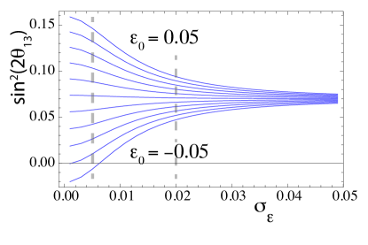
Figure 4: The best fit value of $\sin^{2}(2\theta_{13})$ as a function of the pull-parameter uncertainty $\sigma_{\epsilon}$ for different $\epsilon_{0}$ ranging from -0.05 to 0.05 in steps of 0.01. The transparent dashed vertical lines cutting across the plot indicates the values used to make the two panels of Figure 5

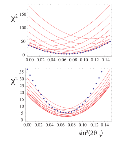
Figure 5: High sensitivity of the $\chi^{2}-pull$ method to small parameters. Both panels show $\chi_{eff}^{2}$ as a function of $s_{213}^{2}$. Upper panel: $\sigma_{\eta}=0.1$ and $\sigma_{\epsilon}=0.005$. Lower panel: $\sigma_{\eta}=1$ and $\sigma_{\epsilon}=0.02$. The dots are $\chi^{2}$ of the simple model, Eq. 1.

Figure 5 shows $\chi_{eff}^{2}$ as a function of $s_{213}^{2}$ with all other parameters floating to their minimizing values. As above the different curves are $\epsilon_{0}$ ranging from -0.05 to 0.05 in steps of 0.01. The upper panel plot uses $\sigma_{\eta}=0.1$ and $\sigma_{\epsilon}=0.005$, the region of large dispersion in Figure 4. Such a small value of $\sigma_{\epsilon}$ tends to prevent the parameters from improving $\chi^{2}$. That is shown by the dots along the bottom of the plot, which represent the fit to the simple model, Eq. 1. Most of the envelope of $\chi^{2}$ values tend to be bounded above the simple model. We find this is significant.

The lower panel of Figure 5 shows the same plot when $\sigma_{\eta}=1$ and $\sigma_{\epsilon}=0.02$. Those choices allows greater freedom for $\eta_{d}$ to improve the fit. Actually the improvement in $\chi^{2}$ from this parameter is marginal. However there is a dramatic change in the width of the plot (and the precision $\Delta s_{213}^{2}$) compared to the other case. Despite the importance of $\sin^{2}(2\theta_{13})$ and its uncertainty, we have seen no specific discussion of the wide range of results that can be obtained simply by adjusting the pull-width parameters. Our hypothesis to fit data with the method must be abandoned because the range of possible values we can find greatly exceeds the range of any error bars from the same analysis.

III.3 Sensitivity Explained: Built-In Degeneracies

Once the pull-width parameters are set somehow, attention shifts to the change in $\chi^{2}$ from varying pull parameters near the minimum. A lack of sensitivity of $\chi^{2}$ has been promoted as a virtue. Actually it is a symptom of analysis degrading resolution.

Consider a general function $\chi^{2}(\theta)$ depending on parameters $\theta=\theta_{1}...\theta_{n}$. Find the best fit points with $\partial\chi^{2}/\partial\theta_{i}=0$ at $\theta=\theta_{*}$. The curvature at $\theta_{*}$ is $\alpha_{ij}={\frac{1}{2}}(\partial\chi^{2}/\partial\theta_{i}\partial\theta_{j})_{\theta_{*}}$. The value of $\chi^{2}$ and its curvature depend on the number of terms and parameters. For example, RENO’s formula reno for $\chi^{2}$ has 12 terms and 12 parameters, possibly explaining why the minimum $\chi^{2}$ shown in the paper’s Figure 3 is zero. When there are even more parameters than terms to be fit, then $\chi^{2}$ must be totally insensitive to certain linear combinations of the parameters. Insensitivity means the curvature eigenvalues will be unusually small from built-in near degeneracies. But it is not strictly necessary to have more parameters than terms. It is sufficient for the nature of the parameters to nearly reproduce one another to produce built-in near degeneracies.

The covariance matrix $C_{ij}=(\alpha^{-1})_{ij}$ has the inverse eigenvalues. It defines the standard uncertainty of fit parameters. For example the uncertainty of $\theta_{1}$ when $\chi^{2}$ varies by $\Delta\chi^{2}$ in a one-parameter variation is $\sqrt{C_{11}\Delta\chi^{2}}$. Inverting matrices with a large ratio of maximum eigenvalues ($\lambda_{max}$) to minimum eigenvalues ($\lambda_{min}$) is unstable, also called “ill-conditioned”. An ill-conditioned inverse has inordinate sensitivity to small projections of parameters along the eigenvectors with small eigenvalues. The cure for ill-conditioned problems removes the subspace of $a_{ij}$ labeled by eigenvalues below some $cut$ value by inverting the matrix in the complementary subspace, forming the pseudoinverse $C_{cut}$. In symbols

$$\alpha =\sum_{\alpha}^{K}\,|a_{\alpha}>\lambda_{\alpha}<a_{\alpha}|;$$

$$C_{cut} =\sum_{\alpha}\,\theta(\lambda_{\alpha}/\lambda_{max}>cut)|a_{\alpha}>(\lambda_{\alpha})^{-1}<a_{\alpha}|.$$

The step function $\theta(\lambda_{\alpha}/\lambda_{max}>cut)$ enforces the eigenvalues $\lambda_{\alpha}$ are larger than the fraction $cut$ of the largest eigenvalue $\lambda_{max}$.

Figure 6 shows how the relative uncertainty $\Delta s_{213}^{2}/s_{213}^{2}$ depends on the ratio $logcut=-\log_{10}(\lambda_{max}/\lambda_{min})$. (For simplicity $\Delta\chi^{2}=1$; the calculation can be trivially rescaled for a more conventional value.) Note the logarithmic scale. The calculation uses $\sigma_{\eta}=1$, $\sigma_{\epsilon}=0.01$, and explores the range $-0.05\leq\epsilon_{0}\leq 0.05$ in steps of 0.01. The steps in $\Delta s_{213}^{2}/s_{213}^{2}$ come at the $logcut$ values where an eigenspace and its corresponding contribution to the calculation is removed. Very tiny variations produce sudden and large effects, the classical signal of an ill-conditioned problem. Many cases of $\chi^{2}-pull$ that we investigated were ill-conditioned.

That explains the “paradox” cited in the introduction: the high sensitivity of fitted results to external parameters is found precisely in the insensitivity of $\chi^{2}$ values to an excessive number of variationally-fit parameters. Our investigation has found that using too many parameters creates an ill-conditioned, insensitive procedure that actually decreases the resolution of $\sin^{2}(2\theta_{13})$. A simpler analysis targeted on the physical parameter $s_{213}^{2}$ must necessarily improve the precision of its determination. For illustration of this, compare the simple straightforward model of Section II.

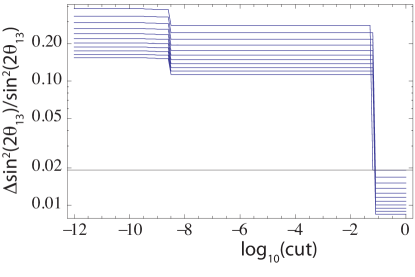
Figure 6: A case of high sensitivity of the $\chi^{2}-pull$ method explained. The figure shows the relative uncertainty $\Delta s_{213}^{2}/s_{213}^{2}$ evaluated as a function of the $logcut=\log_{10}(\lambda_{min}/\lambda_{max})$, where $\lambda_{min}$ and $\lambda_{max}$ are the minimum and maximum eigenvalues retained in making the covariance matrix. Different curves represent $\epsilon_{0}$ ranging from -0.05 to 0.05 in steps of 0.01.

IV Summary

We began this study as a sort of detective investigation to discover what had been done with neutrino reactor data. Our initial impression was that straightforward data analysis took maximum advantage of the new technology of identical detectors. Actually we found that the analysis methods in wide use, by becoming so complicated, have not come close to optimizing the precision of $s_{213}^{2}$.

What is gained by a multi-parameter fit? Compared to our simple fit, the accomplishment from 18 additional parameters used by $DB$ is a change of $\chi^{2}$ by 1.3 units. Suppose one finds a logical argument (which we’ve not seen) for classifying all parameters as irrelevant nuisances, except the mixing angle of great interest. Then using $\chi_{1}^{2}$ to evaluate $\Delta\chi^{2}$ would be appropriate. Meanwhile the hidden penalty of 18 extra parameters tends to decrease the precision of $s_{213}^{2}$, not increase it. We don’t find that necessary or welcome.

Multi-parameter studies are common in simulating and de-bugging hardware. We believe the information from Daya Bay’s 20 parameter fit is that numerous parameters that might have detected significant systematic errors were found to be small. This is a guess about parameter information those in the field need to know. (The facts are actually unknown so long as the full set of fitting parameters is unavailable.) If the guess regarding systematic errors is correct, it is a wonderful result indicating brilliantly constructed hardware. Physicists interested in neutrino physics know and expect that internal studies of hardware systematics might involve 10 or 20 or 100 parameters laboriously checked and double-checked. And this is supposed to be done before “opening the box” to look at the physical parameter of interest. There is no logical necessity to mix the two different goals. Indeed it would be disappointing if the level of analysis of systematic errors by $DB$ and RENO consisted solely of the unconvincing method (in our opinion) of $\chi^{2}-pull$ presented in published work.

To reiterate this, our analysis finds that a hardware study is far from the best way to fit $s_{213}^{2}$. Once systematic errors are known independently and with good reliability to be small, a few-parameter method tends to be a more effective way to evaluate $s_{213}^{2}$ and its errors. This, and the previous material, explain the remark earlier that the errors in $s_{213}^{2}$ can be viewed as both under-estimated and over-estimated. If outsiders to the experiment were to present a 20-parameter fit, we believe no credence would be given unless the results were assessed with $\chi_{20}^{2}$, if not an even more demanding standard. The significance of detecting $s_{213}^{2}\neq 0$ with 32 units of $\Delta\chi^{2}$ would then be reduced to an equivalent $2\sigma$ effect, and errors computed using $\Delta\chi^{2}=1$ would be considered under-estimated. Meanwhile using 20 parameters has also so flattened the $\chi^{2}$ function by near degeneracies, that it has diluted the impact of data on the measurement. On that basis it is an approach wastefully over-estimating the errors of the competing physical parameter.

We found $s_{213}^{2}=0.07\pm 0.018$ with $\chi^{2}=5.66$ at $\epsilon=-0.002$. On its face this is a better fit than $DB$’s. Our result is illustrative and certainly not the last word, but it strongly suggests that even better methods must exist. It would be good for the experimental groups to present straightforward, simple fits where all definitions are complete, all variables are reported, data is divulged, and results are reproducible. Simplicity and transparency will greatly assist the main interest in neutrino data, which is the comparison of experiments with competing models of the underlying physics.

Acknowledgements: We thank Daya Bay collaboration members J. Cao, K. Heeger, P. Huber, W. Wang and K. Whisnant for information about the experiment and the analysis procedures. We also thank Danny Marfatia for helpful information. Research supported in part under DOE Grant number DE-FG02-04ER14308. ANK thanks Professor F. Tahir for consultation and advice, the University of Kansas Theory Group for kind hospitality, the Higher Education Commission of Pakistan for support for graduate studies and travel under the Indigenous Ph.D. Fellowship Program Batch-IV and International Research Support Initiative Program.

V Appendix: Extracting Data

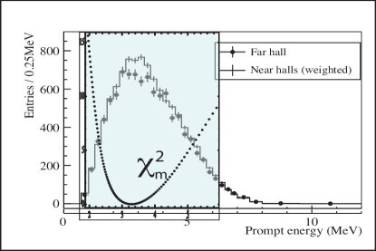
Figure 7: Goodness of fit $\chi_{m}^{2}$ between a 2-parameter oscillation model and the curve of Figure 2 is shown as dots. The horizontal axis is the neutrino energy $E$ in MeV. The histogram and points with error bars are the neutrino energy spectrum from Figure 5 of Ref db1 , superposed with its scale. The minimum of $\chi^{2}_{m}$ at the peak of the energy spectrum is a consistency check that also effectively finds $\Delta m_{13}^{2}=2.32\times 10^{-3}eV^{2}$.

The definitions of quantities and their values accompanying Eq. 2 are taken directly from the experimental report db1 ; db2 . The reports may appear to define everything, but the information is incomplete. We use the following strategy to fill in gaps. From its usage $T_{d}\propto<1-\sin^{2}2\theta_{13}<\sin^{2}(\Delta m_{31}^{2}L_{d}/E)>/L_{d}^{2}$, where the reactor-detector separation is $L_{d}$ and the angle-brackets represent an average over the reactor spectrum multiplied by the cross section and acceptance . Those details might seem to preclude any challenge. Fortunately the effective survival probability $P_{eff}$ for $DB$ is given in the paper’s Figure 4, reproduced here as Fig. 2. The red curve shows the fraction $P_{d}$ of neutrinos surviving at best fit. It is important that the curve already includes all reactor and detector effects: flux, distance, acceptance, live time, efficiency, backgrounds, etc.

Using $P_{d}$ and the expected events listed in $DB$’s Table II produced our Table I. There are other ways to proceed. $DB$ lists inverse beta decay candidate event rates per day, live times, and some background figures. Combining those number produces numbers close to those of Table I, but not exactly the same. Since we are making points of principle and procedure the exact numbers are important but not crucial. For one thing, $DB$’s description of efficiencies and “simulations” are not described in enough detail to reproduce their values.

Digitizing the $P_{d}$ curve in Fig. 2 and fitting it produces

$$P_{eff}(L_{eff},\theta,\mu)=1-\sin^{2}(2\theta)\sin^{2}(\mu L_{eff}/km),$$

where $\sin^{2}(2\theta)=0.0762$, $\mu=0.894$. Here $L_{eff}$ is the effective distance defined in computing the curve. For the entire range covering the data the differences of the 2-parameter fit from the curve are less than the thickness of the curve. (Actually, we only need the $L_{eff}$ dependence and $P_{d}$ evaluated at the detector positions. The good quality of the curve fit is a consistency check.)

As a further check, recall that mono-energetic neutrinos of energy $E$ mixing by one angle predict $\mu=1.267(\Delta m_{13}^{2}/eV^{2})E/GeV$. Using $\Delta m_{13}^{2}=2.32\times 10^{-3}eV^{2}$ translates the 2-parameter fit into an acceptance-averaged energy of $E=3.3$ MeV. It is quite significant that this average energy precisely matches the peak of the spectrum, as shown in Figure 7. To make the figure we defined $\chi_{m}^{2}(E)$ by summing the differences of squares of the curve and fit over 141 digitized values, and finally multiplying by an arbitrary factor of 100 to make the values visible. This approach to fitting $\mu$ also finds $\Delta m_{13}^{2}$ independently using the $DB$ data . The data shown by the probabilities in Fig. 2 detector-by-detector is now ready to be fit.

References

- (1) F. An et al. (Daya Bay Collaboration), Phys. Rev. Lett. 108, 171803 (2012).
- (2) F. An et al. (Daya Bay Collaboration), Chin. Phys. C37, 011001 (2013); Ibid arXiv:1310.6732 [hep-ex].
- (3) K. Ahn et al. (RENO Collaboration), Phys. Rev. Lett. 108, 191802 (2012).
- (4) B. Pontecorvo, Zh. Eksp. Theo. Fiz. 34, 247 (1957) [Sov. Phys. JETP 7, 172 (1958)].
- (5) Z. Maki, M. Nakagawa, and S. Sakata, Prog. Theor. Phys. 28, 870 (1962).
- (6) M. Apollonio et al. (CHOOZ Collaboration), Phys. Lett. B466, 415 (1999); Eur. Phys. J. C27, 331 (2003).
- (7) Y. Abe et al. (Double Chooz Collaboration), Phys. Rev. Lett. 108, 131801 (2012).
- (8) Y. Abe et al. (Double Chooz Collaboration), Phys. Rev. D 86, 052008 (2012).
- (9) Y. Abe et al. (Double Chooz Collaboration), Phys. Lett. B 723, 66 (2013); arXiv:1301.2948v1 [hep-ex], (2013).
- (10) A. N. Khan, D. W. McKay and J. P. Ralston, arXiv:1307.3299.
- (11) X. Guo et al. [Daya-Bay Collaboration], hep-ex/0701029.
- (12) G. Fogli, E. Lisi, A. Marrone, D. Montanino, A. Pallazo, Phys. Rev. D, 66, 053010 (2002).
- (13) S. Fukuda et al. [The Super-Kamiokande Collaboration], Phys. Rev. Lett. 86, 5651-5655 (2001).
- (14) A. Strumia and F. Vissani, JHEP 0111, 048 (2001).
- (15) A. de Gouvea, A. Friedland, H. Murayama, JHEP 103, 009 (2001); (hep-ph/9910286).
- (16) P. Huber, M. Lindner, T. Schwetz, W. Winter, Nuclear Physics B 665, 487 (2003).
- (17) D. Stump et al., Phys. Rev. D 65, 014012 (Appendix B) (2001).
- (18) H. Minakata and H. Nunokawa, JHEP 10, 001 (2001)
- (19) Gomez-Cadenas, P. Hernandez, O. Mena, Nucl. Phys. B 608, 301 (2001); hep-ph/0103258.
- (20) V. Barger, D. Marfatia, K. Whisnant, Phys.ÊRev. D 65, 073023 (2002); hep-ph/0112119.
- (21) P. Huber, M. Lindner, W. Winter, Nucl. Phys. B bf 645 (2002) 3, hep-ph/0204352.
- (22) J. Beringer et al. (Particle Data Group), Phys. Rev. D 86, 010001 (2012).
- (23) Numerical Recipes: The Art of Scientific Programming, W. Press, S. Teukolsky, W. Vetterling and B. Flannery, 3rd Edition, Cambridge University Press, 2007.
- (24) Y. Fukuda et al. [Super-Kamiokande Collaboration], Phys. Rev. Lett. 81, 1562 (1998) [hep-ex/9807003].
- (25) Y. Ashie et al. [Super-Kamiokande Collaboration], Phys. Rev. D 71, 112005 (2005) [hep-ex/0501064].
- (26) K. Abe et al. (T2K Collaboration), Phys. Rev. Lett. 107, 041801 (2011).
- (27) P. Adamson et al. (MINOS Collaboration), Phys. Rev. Lett. 107, 181802 (2011).
- (28) G. Feldman and R. Cousins, Phys. Rev. D 57, 3873 (1998).
- (29) In the course of this research, we checked over a period of several months with helpful Daya Bay Collaboration members, and it was confirmed that 20 parameters are indeed used and the error is evaluated with parameters floating to their best-fit values.