Generalized Fermat’s principle and action for light rays in a curved spacetime

Abstract

We start with formulation of the generalized Fermat’s principle for light propagation in a curved spacetime. We apply Pontryagin’s minimum principle of the optimal control theory and obtain an effective Hamiltonian for null geodesics in a curved spacetime. We explicitly demonstrate that dynamical equations for this Hamiltonian correctly reproduce null geodesic equations. Other forms of the action for light rays in a curved spacetime are also discussed.

I Introduction

It is well known that the Maxwell equations in a curved spacetime can be written in the form of the electromagnetic field equations in a flat space-time in the presence of a medium with the dielectric permittivity and magnetic permeability tensors related to the spacetime metric Pleb ; VoIzSk ; Mash . In the geometric optics approximation the problem of propagation of high frequency electromagnetic waves is reduced to study the geometry of null geodesics, that play the role of bi-characteristics for the wave fronts. Thus this problem is similar to ordinary optics in the media. Fermat’s principle proved to be a useful tool for study this problem BoWo . The Fermat’s principle for light propagation in a static spacetime was formulated in Weyl ; Pauli ; MTW . Its generalization to a stationary spacetime was given in the book by Landau and Lifshitz LL and later in a nice paper by Brill Brill . Fermat’s principle basically states, that a light ray from a spatial point 1 to a point 2 propagates along such a path that takes the least time. Recently Kovner Kovner proposed a generalization of the Fermat’s principle which is valid for light rays in an arbitrary (not necessary stationary) spacetime. According to this principle the arrival time of a future directed null ray emitted from some point 1 and registered by an observer, moving along any timelike worldline, is stationary (minimal) for a null geodesic. A simple derivation of this result was given in NiSa . A comprehensive discussion of the generalized Fermat’s principle can be found in the papers by Perlick Pe:90a ; Pe:90b . He also formulated an action for light rays in an arbitrary metric based on the Fermat’s principle Pe:90a .

In the present paper we propose a slightly different approach for study light rays in a curved $(n+1)-$dimensional spacetime based on the Fermat’s principle. One can foliate the spacetime region by a $n-$parameter family of timelike curves. The coordinates $x^{i}$, ‘enumerating’ this curves can be used as coordinates in a reduced $n-$dimensional space $\Gamma^{n}$. Any $n-$dimensional curve connecting an initial point $x^{i}_{1}$ with an end point $x^{i}_{2}$ in $\Gamma^{n}$ can be uniquely lifted as a future directed null curve in $(n+1)-$dimensional spacetime $M^{n+1}$, provided one fix time $x^{0}_{1}$ of its emission. Time $x^{0}_{2}$ of the null ray arrival to the end point $x_{2}^{i}$ is a functional of the spatial path. Finding minimal value of this functional is a standard problem of the optimal control theory (see e.g. PePl ; SuWi ; Young . To solve this problem one can use the Pontryagin’s minimal principle Pont . In this paper we use this approach to construct the effective Hamiltonian, and demonstrate that corresponding dynamical equations are equivalent to the equations derived from Perlick’s action Pe:90a and correctly reproduce null geodesic equations in the spacetime $M^{n+1}$.

II Motivation

An action for a particle motion in an external gravitational field in the spacetime $M^{n+1}$ can be written in the form

$$S = \int_{\lambda_{1}}^{\lambda_{2}}d\lambda L\,,$$ (1)

$$L = {1\over 2}\left[\eta^{-1}g_{\mu\nu}{dx^{\mu}\over d\lambda}{dx^{\nu}\over d\lambda}-m^{2}\eta\right]\,.$$ (2)

Here $\mu,\nu=0,1,\ldots,n$, $g_{\mu\nu}$ is the metric, $x^{\mu}(\lambda)$ is a path of a particle and $m$ is its mass. $\eta(\lambda)$ is a Lagrange multiplier, which under the change of the parametrization $\lambda\to\tilde{\lambda}(\lambda)$ transforms as follows

$$\tilde{\eta}d\tilde{\lambda}=\eta d\lambda\,,$$ (3)

so that the action Eq.(1) is reparametrization invariant. The variation of the action is

$$\delta S = -\int_{\lambda_{1}}^{\lambda_{2}}d\lambda\left[{D\over d\lambda}\left(\eta^{-1}{dx^{\mu}\over d\lambda}\right)\delta x_{\mu}\right.$$ (4)

$$+ \left.{1\over 2}\left(\eta^{-2}g_{\mu\nu}{dx^{\mu}\over d\lambda}{dx^{\nu}\over d\lambda}+m^{2}\right)\delta\eta\right]$$

$$+ \left.\left(\eta^{-1}g_{\mu\nu}{dx^{\nu}\over d\lambda}\delta x^{\mu}\right)\right|_{\lambda_{1}}^{\lambda_{2}}\,.$$ (5)

Here $D/d\lambda$ is a covariant derivative in the direction $dx^{\mu}/d\lambda$. For an extremum of the action the following conditions are to be satisfied:

$${D\over d\lambda}\left(\eta^{-1}{dx^{\mu}\over d\lambda}\right)=0\,,$$ (6)

$$g_{\mu\nu}{dx^{\mu}\over d\lambda}{dx^{\nu}\over d\lambda}=-\eta^{2}m^{2}\,,$$ (7)

$$\left.\left(\eta^{-1}g_{\mu\nu}{dx^{\mu}\over d\lambda}\delta x_{\mu}\right)\right|_{\lambda_{1}}^{\lambda_{2}}=0\,.$$ (8)

$\eta(\lambda)$ is an arbitrary function, depending on the choice of the parametrization. After variations, one can always put it equal to 1. For this choice one gets an affine parametrization. The last condition determines, what is called the ‘natural boundary conditions’ Cour ; Gelf .

Let us compare cases of massive and massless particles. To illustrate an important difference between these two cases let us assume that the spacetime is 4-dimensional and flat, that is $g_{\mu\nu}=\eta_{\mu\nu}=\mbox{diag}(-1,+1,1,1)$. Let us fix an initial point $x^{\mu}(\lambda_{1})=x_{1}^{\mu}$. For the massive case the conditions (6) and (7) imply that a curve is timelike geodesic, that is, it is a straight line in the interior of the future null cone $N$ with the vertex at $x_{1}^{\mu}$. It is evident that for any choice of the end point $x^{\mu}(\lambda_{2})=x_{2}^{\mu}$ within $N$ there exist only one timelike geodesic connecting it with $x_{1}^{\mu}$. This means that for $m\neq 0$ a variational problem with fixed end points is well defined and has a unique solution.

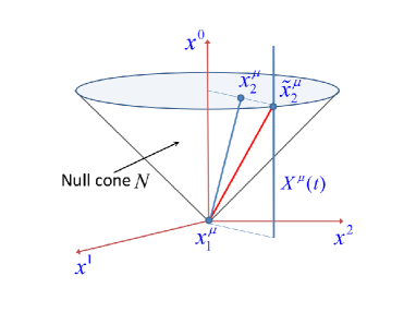
Figure 1: Illustration to variation problem for geodesics in a flat spacetime. $x_{1}^{\mu}$ is a fixed initial point. For a massive particle for any end point $x_{2}^{\mu}$ inside the null cone $N$ there exists a unique solution. For a massless case the end point must lie on the surface of the null cone $N$ (point $\tilde{x}_{2}^{\mu}$). For such a problem one can only require that the end point of the geodesic is at some timelike curve $X^{\mu}(t)$.

In the massless case the situation is quite different. The conditions (6) and (7) imply that a curve is a null geodesic, and hence it is a generator of the null cone $N$ emitted from $x_{1}^{\mu}$. A solution of the problem with a fixed end point exists only when the end point is on this null cone $N$, that is on a special submanifold of dimension 3. The measure of this submanifold is zero. Hence, for a generic choice of the end point $x^{\mu}(\lambda_{2})=x_{2}^{\mu}$ a solution of the variational problem with fixed end points does not exist. In order to have a well defined variational problem for the massless case one may allow the end point not to be fixed but to belong, for example, to a timelike curve. The simplest choice is a straight line

$$X^{\mu}(\tau)=V^{\mu}\tau+B^{\mu}+x^{\mu}_{1}\,,\hskip 14.22636pt{\mbox{\boldmath$V$}}^{2}=-1\,.$$ (9)

This is a trajectory of an observer moving with constant 4-velocity $V^{\mu}$. It crosses the future null cone $N$ emitted at $x^{\mu}_{1}$ at his/her proper time $\tau_{+}$

$$\tau_{+}=\sqrt{{\mbox{\boldmath$B$}}^{2}+({\mbox{\boldmath$V$}},{\mbox{\boldmath$B$}})^{2}}+({\mbox{\boldmath$V$}},{\mbox{\boldmath$B$}})\,.$$ (10)

It is evident that a similar modification of the boundary value problem for the massive particle, when the end point belongs to a timelike line, does not give a unique solution. Any point of $X^{\mu}(\tau)$ for $\tau>\tau_{+}$ can be connected by a timelike geodesic with the initial point $x_{1}^{\mu}$. Hence, instead of a unique solution one would have a one-parameter family of such solutions. To summarize, the variational problems for massive and massless particles are quite different, and one cannot obtain the latter by simply taking the limit $m\to 0$ in the action.

III Generalized Fermat’s principle

Let us consider variational problem for null rays in an arbitrary $(n+1)-$dimensional curved spacetime $M^{n+1}$. We shall not deal with cases when there is more than one geodesics connecting two chosen point. This and other global aspects of the problem are beyond the scope of this paper. In this sense, the following consideration is local. Consider a $n-$dimensional set of timelike curves $x^{\mu}=x^{\mu}(\tau,x^{i})$, where a line is specified by a condition $x^{i}=\mbox{fixed}$ and $\tau$ is a proper time parameter along the curve. We assume that only one line of this set passes through each point in the domain under the consideration. In other words one has a foliation of this domain by $n-$dimensional family of timelike curves. We denote by $V^{\mu}$ vectors tangent to these curves $V^{\mu}=\partial x^{\mu}/\partial\tau$. In the coordinates $(\tau,x^{i})$ the spacetime metric is of the form

$$dS^{2}=-(d\tau-g_{i}dx^{i})^{2}+\gamma_{ij}dx^{i}dx^{j}\,.$$ (11)

We assume that Greek indices, $\mu,\nu,\ldots$ take values $0,1,\ldots n$, while the Latin indices, $i,j,\ldots$ take values $1,2,\ldots n$. Consider a null curve $x^{\mu}(\lambda)$ and denote by $l^{\mu}$ a tangent vector to it, $l^{\mu}=dx^{\mu}/d\lambda=(\dot{x}^{0},\dot{x}^{i})$. We denote by a dot a derivative of a function of $\lambda$ with respect to its argument. A condition that the curve is null, $l_{\mu}l^{\mu}=0$, takes the form

$$-(\dot{\tau}-g_{i}\dot{x}^{i})^{2}+\gamma_{ij}\dot{x}^{i}\dot{x}^{j}=0\,.$$ (12)

A solution of this equation for $\dot{\tau}>0$ is

$$\dot{\tau}=g_{i}\dot{x}^{i}+U\,,\hskip 14.22636ptU=\sqrt{\gamma_{ij}\dot{x}^{i}\dot{x}^{j}}\,.$$ (13)

Let $x^{i}=x^{i}(\lambda)$ be a curve in space $\Gamma^{n}$ with coordinates $x^{i}$. Equation (13) allows one to lift it to the spacetime $M^{n+1}$ as a null curve $x^{\mu}(\lambda)$. It is sufficient to choose the value of $\tau$ at the initial point, $\tau(\lambda_{1})=\tau_{1}$, and solve ODE (13) with this initial data.

Consider a 1-parameter family of curves $x^{i}(\lambda,\varepsilon)$ connecting an initial point $x^{i}_{1}$ and a final point $x^{i}_{2}$ in the space $\Gamma^{n}$, so that

$$x^{i}(\lambda_{1},\varepsilon)=x^{i}_{1}\,,\hskip 14.22636ptx^{i}(\lambda_{2},\varepsilon)=x^{i}_{2}\,.$$ (14)

We consider the corresponding 1-parameter family of lifted curves $x^{\mu}(\lambda,\varepsilon)$ in the spacetime $M^{n+1}$ that have the same initial value $x^{0}(\lambda_{1},\varepsilon)=\tau_{1}$. We choose this family so that the lifted $(n+1)-$dimensional curve for $\varepsilon=0$ is a null geodesic. For a given curve $x^{i}(\lambda,\varepsilon)$ from the family, the final value $x^{0}(\lambda_{2},\varepsilon)=\tau_{2}(\varepsilon)$ can be found by solving the equation Eq.(13).

Let us show now that the arrival time $\tau_{2}(0)$ for a null geodesic gives an extremum for a function $\tau_{2}(\varepsilon)$. Let us fix the initial point $x^{\mu}=(\tau_{1},x^{i}_{1})$ and the final $n-$dimensional point $x^{i}_{2}$. Then the action Eq.(1) is a function of $\varepsilon$, $S(\varepsilon)$. When equations (6) and (7) are satisfied, the variation of this function takes the form

$$\delta_{\varepsilon}S=\left.\eta^{-1}g_{\mu\nu}\dot{x}^{\nu}\delta x^{\mu}\right|_{2}=\eta_{2}^{-1}(l_{i}\delta x_{2}^{i}+l_{\tau}\delta\tau_{2})\,.$$ (15)

Since $\delta x_{2}^{i}=0$ and $\eta^{-1}l_{\tau}\neq 0$, the natural boundary conditions (8) imply that

$$\left.{\partial\tau_{2}(\varepsilon)\over\partial\varepsilon}\right|_{\varepsilon=0}=0\,.$$ (16)

To summarize, the light emitted at $x^{\mu}_{1}$ reaches an observer at $x^{i}_{2}$ earlier than any other null curve. This is an evident generalization of the Fermat’s principle for a general case of a curved spacetime.

IV Optimal control approach, Pontryagin’s minimum principle, and an effective Hamiltonian

Using the generalized Fermat’s principle one can formulate the problem of finding light rays in the following way. Consider the following set of first order equations

$${dx^{0}\over d\lambda} = \mathcal{Q}(x^{\mu},u^{i})\,,$$ (17)

$${dx^{i}\over d\lambda} = u^{i}\,$$ (18)

$$\mathcal{Q}(x^{\mu},u^{i}) = g_{i}(x^{\mu})u^{i}+\sqrt{\gamma_{ij}(x^{\mu})u^{i}u^{j}}\,.$$ (19)

We denote by $J$ the following functional

$$J=\int_{x_{1}^{\mu}}^{x_{2}^{i}}d\lambda\mathcal{Q}(x^{\mu}(\lambda),u^{i}(\lambda)\,.$$ (20)

Here and later we use the notation $\int_{x_{1}^{\mu}}^{x_{2}^{i}}d\lambda\ldots$ to indicate that we fix at $\lambda_{1}$ an initial spacetime point $x_{1}^{\mu}$, while at the end point $\lambda_{2}$ we fix only its spatial position $x_{2}^{i}$.

The value of $J$ calculated for a solution of (17)-(19) coincides with $\delta\tau=\tau_{2}-\tau_{1}$. According to the generalized Fermat’s principle the light ray trajectory provides an extremum (minimum) of the functional $J$.

One may consider such a task as a version of a general optimal control problem, by identifying $u^{i}(\lambda)$ with control functions. To solve this problem one introduces the following Hamiltonian Pont ; Hull

$$\mathcal{H}(\psi_{\mu},x^{\mu},u^{i})=\psi_{0}\mathcal{Q}+\psi_{i}u^{i}\,.$$ (21)

The corresponding Hamilton equations are

$${d\psi_{\mu}\over d\lambda} = -{\partial\mathcal{H}\over\partial x^{\mu}}=-\psi_{0}{\partial{\mathcal{Q}}\over\partial x^{\mu}}\,,$$ (22)

$${dx^{0}\over d\lambda} = {\partial\mathcal{H}\over\partial\psi_{0}}=\mathcal{Q}\,,$$ (23)

$${dx^{i}\over d\lambda} = {\partial\mathcal{H}\over\partial\psi_{i}}=u^{i}\,.$$ (24)

According to Pontryagin’s minimum principle one should substitute a solution of these equations for given control functions $u^{i}$ into the effective Hamiltonian $\mathcal{H}$, and after this determine them from the condition that they minimize the value of the Hamiltonian. In our case, when $u^{i}$ are smooth functions, the corresponding conditions are

$${\partial\mathcal{H}\over\partial u^{i}}\equiv\psi_{0}{\partial\mathcal{Q}\over\partial u^{i}}+\psi_{i}=0\,.$$ (25)

When satisfying along the trajectory these equations are necessary condition for an optimum.

A set of equations (22)–(25) can be simplified. In particular, Eq.(25) gives

$$\psi_{i}=-\psi_{0}{\partial\mathcal{Q}\over\partial u^{i}}\,,$$ (26)

while the equations (22)-(24) can be written in the form

$${d\over d\lambda}\left(\psi_{0}{\partial{Q}\over\partial\dot{x}^{i}}\right)-\psi_{0}{\partial{Q}\over\partial{x}^{i}}=0\,,$$ (27)

$${d\psi_{0}\over d\lambda}=-\psi_{0}{\partial{Q}\over\partial{x}^{0}}\,,$$ (28)

$${dx^{0}\over d\lambda}=Q\,.$$ (29)

Here we denote

$$Q = Q(x^{\mu},\dot{x}^{i})=\mathcal{Q}(x^{\mu},u^{i}=\dot{x}^{i})$$ (30)

$$= g_{i}\dot{x}^{i}+U\,,\hskip 14.22636ptU=\sqrt{\gamma_{ij}\dot{x}^{i}\dot{x}^{j}}\,.$$ (31)

Using Eq.(28) to exclude $\psi_{0}$ from Eq.(27) and taking into account Eq.(29) one obtains the following relation

$${d\over d\lambda}\left({\partial{Q}\over\partial\dot{x}^{i}}\right)-{\partial{Q}\over\partial{x}^{i}}-{\partial{Q}\over\partial{x}^{0}}{\partial{Q}\over\partial\dot{x}^{i}}=0\,.$$ (32)

Equations (32) and (29) totally determine a null ray trajectory. It is easy to check that these equations are reparametrization invariant, that is they are invariant under the transformation $\lambda\to\tilde{\lambda}=f(\lambda)$. We shall now explicitly demonstrate that they are equivalent to the $(n+1)-$dimensional geodesic equations for null rays.

V Consistency

V.1 Null geodesics in $M^{n+1}$

Consider a null ray $x^{\mu}(\lambda)$ and denote, as earlier, $l^{\mu}=\dot{x}^{\mu}$ a tangent vector to it. In the metric (11) one has

$$l^{\mu} = (U+g_{i}\dot{x}^{i},\dot{x}^{i})\,,$$ (33)

$$l_{\mu} = (-U,g_{i}U+\gamma_{ij}\dot{x}^{j})\,.$$ (34)

The null geodesic equation in $M^{n+1}$, (6), has the form

$${Dl^{\mu}\over d\lambda}\equiv l^{\nu}l^{\mu}_{;\nu}=\tilde{F}l^{\mu}\,,\hskip 14.22636pt\tilde{F}=\eta^{-2}\dot{\eta}\,.$$ (35)

Here, as earlier, $D/d\lambda$ is the covariant derivative in $l^{\mu}$ direction. We do not assume that $\lambda$ is an affine parameter, so that $\tilde{F}$ does not necessary vanishes.

Let us consider first the relation

$$g_{0\mu}{Dl^{\mu}\over d\lambda}\equiv{Dl_{0}\over d\lambda}=\tilde{F}l_{0}\,.$$ (36)

This equation gives

$${dU\over d\lambda}+\Gamma^{\alpha}_{0\beta}l_{\alpha}l^{\beta}=\tilde{F}U\,.$$ (37)

The expressions for the Christoffel symbols for the metric Eq.(11) are given in the Appendix. After simplifications one obtains the following relation

$${dU\over d\lambda}+Ug_{i,0}\dot{x}^{i}+{1\over 2}\gamma_{ij,0}\dot{x}^{i}\dot{x}^{j}-\tilde{F}U=0\,.$$ (38)

The other null geodesic equations can be written in the form

$$\gamma_{ij}{Dl^{j}\over d\lambda}=\tilde{F}_{i}\,,\hskip 14.22636pt\tilde{F}_{i}=\tilde{F}\gamma_{ij}\dot{x}^{j}\,.$$ (39)

They can be rewritten in the following explicit form

$$\gamma_{ij}{\mathcal{D}^{2}x^{j}\over d\lambda^{2}}+\tilde{B}^{(0)}_{i}+\tilde{B}^{(1)}_{i}U+\tilde{B}^{(2)}_{i}U^{2}=\tilde{F}_{i}\,,$$ (40)

$$\tilde{B}^{(0)}_{i}=g_{i,0}(g_{k}\dot{x}^{k})^{2}+g_{ij,0}\dot{x}^{j}g_{k}\dot{x}^{k}-{1\over 2}g_{i}g_{jk,0}\dot{x}^{j}\dot{x}^{k}\,,$$

$$\tilde{B}^{(1)}_{i}=2g_{i,0}g_{k}\dot{x}^{k}+g_{ij,0}\dot{x}^{j}+2A_{ij}\dot{x}^{j}\,,$$ (41)

$$\tilde{B}^{(2)}_{i}=g_{i,0}\,.$$

We denote by ${\mathcal{D}/d\lambda}$ a $n-$dimensional covariant derivative with respect the metric $\gamma_{ij}$ in the direction $\dot{x}^{i}$

$${\mathcal{D}^{2}x^{j}\over d\lambda^{2}}={d^{2}x^{j}\over d\lambda^{2}}+\mathcal{T}^{i}_{jk}\dot{x}^{j}\dot{x}^{k}\,,$$ (42)

$$\mathcal{T}_{i,jk}={1\over 2}(\gamma_{ij,k}+\gamma_{ik,j}-\gamma_{jk,i})\,,$$ (43)

$$\mathcal{T}^{i}_{jk}=\gamma^{in}\mathcal{T}_{n,jk}\,.$$

Eq.(38) follows from Eq.(41) and the relation

$$\dot{x}^{0}=g_{i}\dot{x}^{i}+U\,.$$ (44)

To show this it is sufficient to multiply Eq.(40) by $\dot{x}^{i}$ and use the relation

$$\gamma_{ij}\dot{x}^{i}{\mathcal{D}^{2}x^{j}\over d\lambda^{2}}=U{dU\over d\lambda}-{1\over 2}\gamma_{ij,0}\dot{x}^{0}\dot{x}^{i}\dot{x}^{j}\,.$$ (45)

Thus, equations (40), (41) and (44) uniquely determine a null geodesic in $M^{n+1}$.

V.2 Hamiltonian equations

Let us now write Eq.(32) in an explicit form. We notice that

$${\partial Q\over\partial\dot{x}^{i}}=g_{i}+{1\over U}\gamma_{ij}\dot{x}^{j}\,,$$ (46)

$${\partial Q\over\partial{x}^{i}}=g_{j,i}\dot{x}^{j}+{1\over 2U}\gamma_{kl,i}\dot{x}^{k}\dot{x}^{l}\,,$$ (47)

$${\partial Q\over\partial{x}^{0}}=g_{i,0}\dot{x}^{i}+{1\over 2U}\gamma_{kl,0}\dot{x}^{k}\dot{x}^{l}\,,$$ (48)

$${d\over d\lambda}{\partial Q\over\partial\dot{x}^{i}}=g_{i,0}(g_{k}\dot{x}^{k}+U)+g_{i,j}\dot{x}^{j}$$

$$-{1\over U^{2}}{dU\over d\lambda}\gamma_{ij}\dot{x}^{j}+{1\over U}\gamma_{ij,0}\dot{x}^{j}(g_{k}\dot{x}^{k}+U)$$ (49)

$$+{1\over U}(\gamma_{ij,k}\dot{x}^{j}\dot{x}^{k}+\gamma_{ij}\ddot{x}^{j})\,.$$

Using these relations and Eq.(29) one can show that Eq.(32) is equivalent to the following equations

$$\gamma_{ij}{\mathcal{D}^{2}x^{j}\over d\lambda^{2}}+B^{(0)}_{i}+B^{(1)}_{i}U+B^{(2)}_{i}U^{2}=F_{i}\,,$$ (50)

$$B^{(0)}_{i}=g_{k}\dot{x}^{k}\gamma_{ij,0}\dot{x}^{j}-{1\over 2}g_{i}\gamma_{jk}\dot{x}^{j}\dot{x}^{k}\,,$$

$$B^{(1)}_{i}=g_{i,0}g_{k}\dot{x}^{k}+\gamma_{ij,0}\dot{x}^{j}-g_{i}g_{k,0}\dot{x}^{k}+2A_{ij}\dot{x}^{j}\,,$$ (51)

$$B^{(2)}_{i}=g_{i,0}\,,\hskip 14.22636ptF_{i}=F\gamma_{ij}\dot{x}^{j}\,,$$

$$F={1\over U}{dU\over d\lambda}-g_{k,0}\dot{x}^{k}-{1\over 2U}\gamma_{kl,0}\dot{x}^{k}\dot{x}^{l}\,.$$ (52)

By comparing Eq.(41) and Eq.(51) and using relation $g_{ij}=\gamma_{ij}-g_{i}g_{k}$ one can see that the coefficients in equations (40) and (50) are identical, namely

$$\tilde{B}^{(0)}_{i}=B^{(0)}_{i}\,,\hskip 14.22636pt\tilde{B}^{(1)}_{i}=B^{(1)}_{i}\,,\hskip 14.22636pt\tilde{B}^{(2)}_{i}=B^{(2)}_{i}\,.$$ (53)

To have identical right hand sides of this equations one must put $\tilde{F}=F$. This condition guarantees that in the both cases the parametrization $\lambda$ is identical.

To summarize, we demonstrated that equations (32) and (29), obtained from the Hamiltonian Eq.(21), are equivalent to the equations (35) for a null geodesic in $M^{n+1}$.

VI Perlick’s form of the action

Perlick Pe:90a proposed an elegant form of the action for null rays. Its slightly modified version is

$$\mathcal{S}[x^{\mu}(\lambda),\mu(\lambda)]=\int_{x_{1}^{\mu}}^{x_{2}^{i}}d\lambda\ \mathcal{L}\,,$$ (54)

$$\mathcal{L}=\mu(\lambda)(\dot{x}^{0}-Q)\,,$$ (55)

$$Q=g_{i}\dot{x}^{i}+U\,,\hskip 14.22636ptU=\sqrt{\gamma_{ij}\dot{x}^{i}dx^{j}}\,.$$ (56)

Here $\mu(\lambda)$ is a Lagrange multiplier. The action is invariant under the reparametrization $\lambda\to\tilde{\lambda}(\lambda)$, provided $\mu$ is not transformed, $\tilde{\mu}=\mu$. Variations of this action give the following equations

$${\delta\mathcal{S}\over\delta\mu} \equiv \dot{x}^{0}-Q=0\,,$$ (57)

$$-{\delta\mathcal{S}\over\delta x^{0}} \equiv \dot{\mu}+\mu{\partial Q\over\partial x^{0}}=0\,,$$ (58)

$${\delta\mathcal{S}\over\delta x^{i}} \equiv {d\over d\lambda}\left(\mu{\partial Q\over\partial\dot{x}^{i}}\right)-\mu{\partial Q\over\partial x^{i}}=0\,.$$ (59)

It is easy to see that after putting $\mu=\psi_{0}$ this set of equations is identical to equations (27)-(29) obtained from the effective Hamiltonian (21). Hence, as it was shown in the previous section, it correctly reproduces the null geodesic equations in $M^{n+1}$.

Let us denote by $\{\pi,p_{\mu}\}$ momenta conjugated to $\{\mu,x^{\mu}\}$

$$\pi = {\partial\mathcal{L}\over\partial\dot{\mu}}=0\,,$$ (60)

$$p_{0} = {\partial\mathcal{L}\over\partial\dot{x}^{0}}=\mu\,,$$ (61)

$$p_{i} = {\partial\mathcal{L}\over\partial\dot{x}^{i}}=-\mu{\partial Q\over\partial\dot{x}^{i}}\,.$$ (62)

The Hamiltonian

$$H^{*}=\pi\dot{\mu}+p_{\mu}dx^{\mu}-\mathcal{L}$$ (63)

identically vanishes. This is a consequence of the reparametrization invariance of the action (54).

Denote

$$\pi_{i}={p_{i}\over p_{0}}\,.$$ (64)

Then one has

$$\pi_{i}=g_{i}+{1\over U}\gamma_{ij}\dot{x}^{j}\,.$$ (65)

It is easy to check that in addition to a trivial constraint (60) the following constraint is satisfied

$$\varphi\equiv{1\over 2}\left[\gamma^{ij}(\pi-g_{i})(\pi_{j}-g_{j})-1\right]=0\,.$$ (66)

These two constraints, (60) and (66), are of the first order, that is they Poisson commute. Following the general theory of dynamical systems with constraints Dirac one should introduce an effective Hamiltonian, which is a linear combination of the constraints

$$H=v\pi+u\varphi\,.$$ (67)

Here $v=v(\lambda)$ and $u=u(\lambda)$.

One has

$${\partial\varphi\over\partial p_{0}}={\partial\varphi\over\partial\pi_{i}}{\partial\pi_{i}\over\partial p_{0}}=-{1\over p_{0}}\pi_{i}{\partial\varphi\over\partial\pi_{i}}\,$$ (68)

$${\partial\varphi\over\partial p_{i}}={\partial\varphi\over\partial\pi_{i}}{\partial\pi_{i}\over\partial p_{i}}={1\over p_{0}}{\partial\varphi\over\partial\pi_{i}}\,$$ (69)

$${\partial\varphi\over\partial\pi_{i}}=\gamma^{ij}(\pi_{i}-g_{i})\,,$$ (70)

$$\pi_{i}{\partial\varphi\over\partial\pi_{i}}=1-g_{i}g^{i}+g^{i}\pi_{i}\,.$$ (71)

The Hamilton equations for Eq.(67) are

$$\dot{\mu} = {\partial H\over\partial\pi}=v\,,$$ (72)

$$\dot{\pi} = -{\partial H\over\partial\mu}=0\,,$$ (73)

$$\dot{x}^{0} = {\partial H\over\partial p_{0}}=-{u\over p_{0}}\pi_{i}{\partial\varphi\over\partial\pi_{i}}=-{u\over p_{0}}\pi_{i}\gamma^{ij}(\pi_{i}-g_{i})\,$$ (74)

$$\dot{x}^{i} = {\partial H\over\partial p_{i}}={u\over p_{0}}{\partial\varphi\over\partial\pi_{i}}={u\over p_{0}}\gamma^{ij}(\pi_{i}-g_{i})\,$$ (75)

$$\dot{p}_{0} = -{\partial H\over\partial x^{0}}=-u{\partial\varphi\over\partial x^{0}}\,,$$ (76)

$$\dot{p}_{i} = -{\partial H\over\partial x^{i}}=-u{\partial\varphi\over\partial x^{i}}\,.$$ (77)

Eq.(73) implies

$$\pi_{i}={p_{0}\over u}\gamma_{ij}\dot{x}^{j}+g_{i}\,.$$ (78)

The constraint equation $\varphi=0$ takes the form

$$-{u\over p_{0}}=U\,.$$ (79)

Thus Eq.(74) can be written in the form

$$\dot{x}^{0}=g_{i}\dot{x}^{i}+U\,.$$ (80)

By combining Eq.(76) and Eq.(77) one obtain

$$\dot{\pi}_{i}=U\left({\partial\varphi\over\partial x^{i}}+\pi_{i}{\partial\varphi\over\partial x^{0}}\right)\,.$$ (81)

Simple calculations give

$${\partial\varphi\over\partial x^{\mu}}=-{1\over 2U^{2}}\gamma_{jk,\mu}\dot{x}^{j}\dot{x}^{k}+{1\over U}g_{j,\mu}\dot{x}^{j}\,.$$ (82)

Straightforward calculations allows one to show that the equations (81) are equivalent to equations (50)-(52).

VII Fermat’s principle in a stationary spacetime

In a stationary spacetime the above considerations are greatly simplified. Let us write the line element in a stationary spacetime with the Killing vector $\xi^{\mu}$ in the form

$$ds^{2} = hdS^{2}\,,\hskip 14.22636pth=-g_{tt}=-{\mbox{\boldmath$\xi$}}^{2}\,,$$ (83)

$$dS^{2} = -(dt-g_{i}dx^{i})^{2}+\gamma_{ij}dx^{i}dx^{j}\,.$$ (84)

Here

$$g_{i}={g_{ti}\over h}\,,\hskip 14.22636pt\gamma_{ij}={g_{ij}\over h}+g_{i}g_{j}\,.$$ (85)

The expression for $dS^{2}$ is similar to Eq.(11) with only one important difference: its coefficient now do not depend on time $t$. We call the metric Eq.(84) ultrastationary. The ultrastationary metric $dS^{2}$ is connected with the physical metric $ds^{2}$ by the conformal transformation. Since both null lines and null geodesics are conformal invariant, one can always reduce the problem in a stationary spacetime to the corresponding problem in the ultrastationary one.

The equation Eq.(32) in the metric Eq.(84) takes the form

$${d\over d\lambda}\left({\partial{Q}\over\partial\dot{x}^{i}}\right)-{\partial{Q}\over\partial{x}^{i}}=0\,.$$ (86)

This is evidently the Euler-Lagrange equation for the action

$$S=\int_{x_{1}^{\mu}}^{x^{i}_{2}}d\lambda(g_{i}\dot{x}^{i}+U)\,.$$ (87)

If null ray is emitted in $x^{i}_{1}$ at $t_{1}$, and arrives to $x^{i}_{2}$ at $t_{2}$, then this action is nothing but the difference $t_{2}-t_{1}$. The condition that that the action is minimal is nothing but a standard Fermat’s principle. This result for stationary spacetimes is well known. Its discussion can be found, for example in LL ; Brill .

Appendix A Useful formulas

For the line element

$$dS^{2}=-(d\tau-g_{i}dx^{i})^{2}+\gamma_{ij}dx^{i}dx^{j}\,.$$ (88)

the metric $g_{\mu\nu}$ and its inverse $g^{\mu\nu}$ are

$$g_{00} = -1\,,\hskip 14.22636ptg_{0i}=g_{i}\,,\hskip 14.22636ptg_{ij}=\gamma_{ij}-g_{i}g_{j}\,,$$ (89)

$$g^{00} = -(1-g_{i}g^{i})\,,\hskip 14.22636ptg^{0i}=g^{i}\,,\hskip 14.22636ptg^{ij}=\gamma^{ij}\,.$$ (90)

We denote by $\gamma^{ij}$ the inverse of the $n-$dimensional metric $\gamma_{ij}$.

We define the Christoffel symbols in $M^{n+1}$ and $\Gamma^{n}$ as follows

$$\Gamma_{\lambda\mu\nu} = {1\over 2}(g_{\mu\lambda,\nu}+g_{\nu\lambda,\mu}-g_{\mu\nu,\lambda})\,,\hskip 5.69046pt\Gamma^{\lambda}_{\mu\nu}=g^{\lambda\alpha}\Gamma_{\alpha\mu\nu}\,,$$ (91)

$$\mathcal{T}_{kij} = {1\over 2}(\gamma_{ik,j}+\gamma_{jk,i}-\gamma_{ij,k})\,,\hskip 5.69046pt\mathcal{T}^{k}_{ij}=\gamma^{kl}\mathcal{T}_{kij}\,.$$ (92)

The components of the Christoffel symbols in $M^{n+1}$ are

$$\Gamma_{000} = 0\,,\hskip 14.22636pt\Gamma_{00i}=0\,,\hskip 14.22636pt\Gamma_{i00}=g_{i,0}\,,$$ (93)

$$\Gamma_{i0j} = {1\over 2}g_{ij,0}+A_{ij}\,,\hskip 14.22636pt\Gamma_{0ij}=-{1\over 2}g_{ij,0}+S_{ij}\,,$$ (94)

$$\Gamma{kij} = \mathcal{T}_{kij}+g_{i}A_{jk}+g_{j}A_{ik}-g_{k}S_{ij}\,.$$ (95)

$$\Gamma^{0}_{00} = g^{i}g_{i,0}\,,\hskip 14.22636pt\Gamma^{i}_{00}=\gamma^{ij}g_{j,0}\,,$$ (96)

$$\Gamma^{0}_{0i} = {1\over 2}g^{j}g_{ij,0}+g^{j}A_{ji}\,,$$ (97)

$$\Gamma^{j}_{0i} = \gamma^{jk}({1\over 2}g_{ik,0}+A_{ki})\,,$$ (98)

$$\Gamma^{0}_{ij} = (1-g_{k}g^{k})({1\over 2}g_{ij,0}+S_{ij})+g^{k}\mathcal{T}_{kij}$$ (99)

$$+ g^{i}g^{k}A_{jk}+g_{j}g^{k}A_{ik}-g_{k}g^{k}S_{ij}\,,$$

$$\Gamma^{k}_{ij} = \mathcal{T}^{k}_{ij}-{1\over 2}g^{k}g_{ij,0}+g_{i}A_{j}^{\ k}+g_{j}A_{i}^{\ k}\,.$$ (100)

We denoted

$$A_{ij}={1\over 2}(g_{i,j}-g_{j,i})\,,\hskip 14.22636ptS_{ij}={1\over 2}(g_{i,j}+g_{j,i})\,.$$ (101)

References

- (1) J. Plebansky, Phys. Rev. 118, 1396 (1960).
- (2) A.M. Volkov, A.A. Izmest ev, and G.V. Skrotskii, JETP 32, 686 (1971).
- (3) B. Mashhoon, Phys. Rev. D 7, 2807 (1973).
- (4) M. Born and E. Wolf Principles of Optics, Pergamon Press, Oxford, England (1970)
- (5) H. Weyl, Annalen der Physik 54, 117 (1917).
- (6) W. Pauli, Theory of Relativity, Pergamon Press, Oxford, England (1958)
- (7) C.W. Misner, K.S. Thorne, and J.A. Wheeler Gravitation, Freemann, San Francisco (1973)
- (8) L.D. Landau and E.M. Lifshitz, The Classical Theory of Fields, Pergamon Press, Oxford, England (1975)
- (9) D. R. Brill, in Relativity, Astrophysics and Cosmology edited by W.Israel (D. Reidel, Dordrecht-Holland, 1973) p. 134.
- (10) I. Kovner, Astrophys. J. 351, 114 (1990).
- (11) R. Nityananda and J. Samuel, Phys. Rev. D 45, 3862 (1992).
- (12) V. Perlick, Classical Quantum Gravity 7, 1319 (1990).
- (13) V. Perlick, Classical Quantum Gravity 7, 1849 (1990).
- (14) H. J. Pesch and M. Plail, Control and Cybernatics, 38 973 (2009).
- (15) H.J. Sussmann and J.C.Willems, IEEE Control Systems, June 1977, p.32.
- (16) L.C. Young, Lectures on Calculus of Variations and Optimal Control Theory, W.B.Saunders Company, Philadelphia-London-Toronto (1969).
- (17) L.S. Pontryagin, V.G. Boltyanskii, R.V. Gamkrelidze, and E.F. Mishchenko The Mathematical Theory of Optimal Processes, John Wiley and Sons, New York (1962)
- (18) R. Courant and D. Hilbert, Methods of Mathematical Physics vol. 1, Interscience Publishers Inc. (1953)
- (19) I.M. Gelfand and S.V. Fomin, Calculus of Variations, Prentice Hall (1963)
- (20) D.G. Hull Optimal Control Theory for Applications, Springer Verlag (2003)
- (21) P.A.M. Dirac Lectures on Quantum Mechanics, Yeshiva University, New York (1964)