Combinatorial theory of the semiclassical evaluation of transport moments II:
Algorithmic approach for moment generating functions

Abstract.

Electronic transport through chaotic quantum dots exhibits universal behaviour which can be understood through the semiclassical approximation. Within the approximation, transport moments reduce to codifying classical correlations between scattering trajectories. These can be represented as ribbon graphs and we develop an algorithmic combinatorial method to generate all such graphs with a given genus. This provides an expansion of the linear transport moments for systems both with and without time reversal symmetry. The computational implementation is then able to progress several orders higher than previous semiclassical formulae as well as those derived from an asymptotic expansion of random matrix results. The patterns observed also suggest a general form for the higher orders.

1. Introduction

The scattering matrix, which connects the asymptotic incoming and outgoing states, conceals the detailed scattering dynamics of the system. Instead the entries encode the transport of states through or across the system. We consider a cavity with two leads attached, so that the scattering matrix separates into reflection and transmission subblocks

(1) $$S(E)=\left(\begin{array}[]{cc}{\boldsymbol{r}}&{\boldsymbol{t}}^{\prime}\\ {\boldsymbol{t}}&{\boldsymbol{r}}^{\prime}\end{array}\right).$$

If the leads carry $N_{1}$ and $N_{2}$ channels respectively, ${\boldsymbol{r}}$ is a square $N_{1}\times N_{1}$ matrix while ${\boldsymbol{t}}$ is $N_{2}\times N_{1}$. We set $N=N_{1}+N_{2}$. The subblocks ${\boldsymbol{r}}$ and ${\boldsymbol{t}}$ encode the electronic transport from one lead to itself or the other respectively. In particular, the eigenvalues of the matrix ${\boldsymbol{t}}^{\dagger}{\boldsymbol{t}}$ are the set of transmission probabilities whose sum is proportional to the average conductance through the cavity [20, 37, 38].

When the cavity is chaotic, the transport properties turn out to be independent of the specifics of the system under consideration. To uncover this universal behavior, two methods have been developed: one involves the semiclassical approximation for the scattering matrix elements in terms of classical trajectories [46, 58, 59], while the other is the random matrix theory (RMT) approach of replacing the scattering matrix with a random one chosen from the appropriate symmetry class [3, 13, 14, 31]. The basic choice is whether the system has time-reversal symmetry (TRS) or not; the corresponding random matrices are the circular orthogonal ensemble (COE) and the circular unitary ensemble (CUE) respectively.

Regardless of the method used, one of the characteristics of the transport properties are the linear moments

(2) $$M_{n}(X)=\left\langle\operatorname{Tr}\left[X^{\dagger}X\right]^{n}\right\rangle,$$

where $X$ can be either the reflection ${\boldsymbol{r}}$ or transmission ${\boldsymbol{t}}$ subblock of the scattering matrix in (1). One can also consider “non-linear” moments, such the as the cross-correlation

(3) $$M_{n_{1},n_{2}}(X_{1},X_{2})=\left\langle\operatorname{Tr}\left[X_{1}^{\dagger}X_{1}\right]^{n_{1}}\operatorname{Tr}\left[X_{2}^{\dagger}X_{2}\right]^{n_{2}}\right\rangle,$$

where $X_{1}$ and $X_{2}$ are again certain sub-blocks of the scattering matrix $S$. Moments involving more products of traces can also be considered. In fact, on the “other side” of the spectrum, in a sense, are the moments

(4) $$M^{k}(X)=\left\langle\left(\operatorname{Tr}X^{\dagger}X\right)^{k}\right\rangle,$$

whose generating function in the CUE case is a special case of the celebrated Harish-Chandra–Itzykson–Zuber (HCIZ) integral [26, 28]

(5) $$I_{N}(z,A,B)=\int_{U(N)}e^{-zN\operatorname{Tr}(AUBU^{\dagger})}\mathrm{d}U.$$

Typically one sets $X$ to be the transmission subblock ${\boldsymbol{t}}$ of the scattering matrix in (1) so that (2) becomes the moments of the transmission eigenvalues and (4) becomes the moments of the conductance.

In the companion paper [11], we showed that the RMT and semiclassical results for any of these moments must be identical. However, while the equivalence has been established, the problem of calculating particular moments is still not fully answered, and remains a hard challenge. There is also a wider class of problems related to energy differentials of the scattering matrix, to systems with superconducting leads attached, and to systems with non-zero Ehrenfest time which can and have also been considered, both semiclassically and within RMT. We review these results in Section 2.

Here we focus mostly on the linear moments in (2), into which we substitute the semiclassical approximation [46, 58, 59]

(6) $$S_{oi}(E)\approx\frac{1}{\sqrt{N\tau_{\mathrm{d}}}}\sum_{\gamma(i\to o)}A_{\gamma}(E)\mathrm{e}^{\frac{\mathrm{i}}{\hbar}S_{\gamma}(E)},$$

involving the scattering trajectories $\gamma$. These trajectories travel from incoming channel $i$ to outgoing channel $o$ with action $S_{\gamma}$ and stability amplitude $A_{\gamma}$ (incorporating the Maslov phase) while $\tau_{\mathrm{d}}$ is the average time spent inside the cavity. The linear moments become the sum

(7) $$M_{n}(X)\sim\left\langle\frac{1}{{(N\tau_{\mathrm{d}})}^{n}}\sum_{{i_{j},o_{j}}}\sum_{\begin{subarray}{c}\gamma_{j}(i_{j}\to o_{j})\cr\gamma^{\prime}_{j}(i_{j+1}\to o_{j})\end{subarray}}\prod_{j=1}^{n}A_{\gamma_{j}}A_{\gamma^{\prime}_{j}}^{*}\mathrm{e}^{\frac{\mathrm{i}}{\hbar}(S_{\gamma_{j}}-S_{\gamma^{\prime}_{j}})}\right\rangle,$$

where $i_{n+1}=i_{1}$ which endows the set of trajectories with a particular structure. Namely, moving forwards along the trajectories $\gamma_{j}$ and backwards along $\gamma^{\prime}_{j}$ we visit the channels $i_{1}\to o_{1}\to i_{2}\ldots o_{n}\to i_{1}$ along a single cycle. For $n=2$ this is depicted in Fig. 1(a).

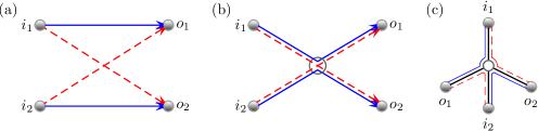
Figure 1. (a) A quadruplet of trajectories that appear in the second linear moment. (b) For the actions to (nearly) cancel, the blue solid and the red dashed trajectories must coincide pairwise along the most part of their length. Nontrivial (but significant) contributions arise when pairs exchange partners by coming close to each other (“crossing”) in encounter regions. (c) A ribbon graph representation of the quadruplet where the encounter becomes a roundabout vertex, links become edges and the trajectories create a boundary walk.

However, to contribute consistently in the semiclassical limit of $\hbar\to 0$, the total action of the set of trajectories should be stationary (under some average). This can be achieved by forcing the trajectories to be nearly identical, except in small regions known as encounters. An example for $n=2$ is given in Fig. 1(b), with the encounter region denoted by the unfilled circle. As detailed in [11] and explained in Section 3 below, the resulting diagram can be interpreted as a ribbon graph, depicted in Fig. 1(c). Edges of the graph correspond to semiclassically long stretches of trajectories following each other in pairs. Vertices of degree $>1$ (“internal vertices”) correspond to encounter regions where two or more pairs of orbits exchange partners. Vertices of degree $1$ (“leaves”) correspond to a pair of trajectories entering or leaving the cavity via a lead.

What is particularly important is that the semiclassical contribution of a diagram can easily be read off from its structure [27, 30, 47, 73]:

Definition 1.

The semiclassical contribution of a diagram is a product where

• every edge provides a factor $1/N$,

• every internal vertex gives a factor of $-N$,

• encounters that happen in the lead do not count (give a factor of $1$).

The diagram in Fig. 1(b) or (c) then gives the contribution

$$\sum_{\begin{subarray}{c}i_{1},i_{2}\cr o_{1},o_{2}\end{subarray}}\frac{-N}{N^{4}},$$

where the result for each channel sum is simply the number of channels in the respective lead. For example, when $X={\boldsymbol{t}}$ the result is $-N_{1}^{2}N_{2}^{2}/N^{3}$, and when $X={\boldsymbol{r}}$, the result is $-N_{1}^{4}/N^{3}$.

With these simple rules, the task of evaluating transport moments semiclassically reduces to that of systematically generating all permissible diagrams. This is itself a formidable problem, and previous incremental progress in its solution is reviewed in Section 2. In this manuscript we present an algorithm that in principle allows one to calculate the generating function

$$\sum_{n=1}^{\infty}s^{n}\operatorname{Tr}\left[X^{\dagger}X\right]^{n},$$

to any required order in the small parameter $1/N$. We stress that the answers obtained are for moments of all orders $n$ at once.

To describe the algorithm we will seek a more detailed understanding of the structure of the semiclassical diagrams contributing at a given order and describe an algebraic method to generate them. The resulting algorithm is implemented on a computer, resulting in an expansion that goes several orders beyond the best of the previously available results [9]. In principle, the algorithm is applicable to any order of $1/N$, but in practice it is severely limited by the available computer capacity.

To classify the contributing orbits we go through several steps. First, after explaining the structure of semiclassical diagrams, we incorporate the contributions of diagrams with encounters in the leads [73] into the contribution of the “principal diagrams” (this method goes back to [6]). This is done in Section 3. Then, in Section 4, we argue that one can obtain diagrams for arbitrary $n$ but fixed order of $1/N$ by grafting a number of trees on the edges and vertices of a “base structure”. Most importantly, the number of such structures is finite for any given order of $1/N$; the structures can be generated automatically from factorizations of permutations as detailed in section 4.1. In Section 5 we obtain the semiclassical contributions of vertices and edges of a base structure; such contributions are essentially the result of a partial sum over all possible trees that can be grafted on the vertex or edge. In Section 6 we present the expressions for the moment generating functions resulting after summation over all base structures at orders $N$ to $N^{-3}$. Conjectures for higher orders are also given.

2. Transport moments

Before turning to a semiclassical method to obtain explicit results for transport moments, we first review some of the previous results in this direction. The body of literature on RMT is immense due to its diverse applications, from number theory to high energy physics (see [2] for a collection of articles reviewing properties and applications of RMT). Here we aim to review the particular results that relate to our main task, to understand the linear moments $M_{n}$ in (2), for large $n$.

2.1. Previous RMT results

The first RMT approaches considered correlators of arbitrary products of matrix elements, which include all the types of moments discussed in the introduction. Averaging over the CUE or the COE, results were obtained [16, 40, 60] in terms of class coefficients or “Weingarten” functions. Although they can in principle be used to calculate any moment, the class coefficients are generated recursively and the results become more unwieldy as the order of the moments increases. The problem became one of finding closed form results for higher moments.

To proceed, Brouwer and Beenakker [16] developed a diagrammatic approach to the random matrix integrals which, aside from recreating previously known results for the conductance and its variance [3, 31], allowed them to obtain the probability distribution (and hence indirectly all the moments) of the transmission eigenvalues at leading and subleading order in inverse channel number. This diagrammatic approach could also be applied to obtain various terms when the scattering matrix is coupled to the leads via a tunnel barrier, or for a normal metal-superconductor junction.

In order to obtain high moments beyond a diagrammatic expansion, a different approach was pioneered by Savin and Sommers [61]. Starting from the probability distribution of the transmission eigenvalues of the matrix ${\boldsymbol{t}}^{\dagger}{\boldsymbol{t}}$ [4, 24] they noted the similarities to the Selberg integral. This allowed them to obtain the second linear moment [61] (related to the shot noise power) and later all linear and non-linear moments up to fourth order [62]. Although moments of this order could still be tractable using the recursive class coefficients, this work spurred a renewal of interest in the RMT treatment of transport moments. For systems without TRS a result for all the linear moments as well as all the moments of the conductance, (4), were obtained using generalisations of the Selberg integral in [50].

The joint probability distribution of the transmission eigenvalues is a particular case of the Jacobi ensemble in RMT [24] which also allowed the linear moments to be calculated for the unitary case using orthogonal polynomial techniques [67] (results using a variation of the Selberg integral were also obtained). The linear moments for all the classical symmetry classes as well as for the superconducting symmetry classes were likewise obtained using orthogonal polynomials [39, 43]. These techniques were also applied to the Laguerre ensemble and the linear moments of the Wigner delay times were calculated [43].

For moments of the type (4), a connection to the theory of integrable systems was exploited to calculate all the moments of the conductance [54] and later the shot noise [55] for systems with broken TRS. The same results, plus the moments for systems with TRS, were obtained using generalised Selberg integrals and symmetric functions [32]. The integrable system approach for the moments of the conductance and shot noise was recently extended to all the classical and superconducting symmetry classes as well as for the moments of the Wigner delay time [45].

Returning to the linear moments of the transmission eigenvalues, in the case of broken TRS there exist several different expressions [39, 43, 50, 67], each involving sums over combinatorial-type terms. The number of terms in the sums increase with the order of the moments leaving high moments difficult to obtain. Interestingly, due to being obtained by different methods, all the results look remarkably different despite encoding the same object. The asymptotic analysis in the limit of a large number of channels $N$ is also challenging, especially beyond the leading order. However, the results of [43] which include systems with TRS are more amenable for such an asymptotic expansion, as detailed in [44].

2.2. Previous semiclassical results

Similar to RMT, on the semiclassical side the low moments were obtained first starting with the conductance [27, 59], the shot noise [15, 63, 73] and then the conductance variance as well as other second order correlation functions [47]. Interestingly, it was the simple result for the shot noise [15] which had not yet been explicitly calculated using RMT which prompted Savin and Sommers to revisit the RMT approach [61]. All these semiclassical results were obtained by mapping the semiclassical diagrams for open systems to those which contribute to the spectral statistics of closed quantum chaotic systems [48, 49, 64]. As the order of the moment increases, this mapping becomes much more complicated, although recently Novaes succeeded in relating this mapping to various combinatorial problems whose solution allows the moments to be generated for systems with broken TRS [51, 52].

Taking a different approach [10, 11] we could show that the contribution of the vast majority of semiclassical diagrams cancel and the remaining diagrams could be identified with primitive factorisations of a permutation. These give results identical to the computation via the class coefficients (Weingarten functions) used for matrix element correlators in RMT [16, 40, 60] and complete equivalence was thus established. This approach works for systems both with and without TRS but provides no further results for the moments. In a separate development, Novaes recently announced a way to generate the diagrams with broken TRS from a matrix integral which he also shows to give the RMT results for arbitrary moments and prove the complete equivalence of semiclassics and RMT [53].

In the quest for computing actual answers, most recent progress came by looking in the direction of high moments but only to the first few terms in the $1/N$ expansion. First it was noticed that the semiclassical diagrams which contribute at leading order to the linear moments could be reinterpreted as trees [6, 7] allowing the moments of the transmission eigenvalues to be generated recursively and encoded in a moment generating function [6]. Including an energy dependence in the semiclassical contributions then allowed access to the leading order density of states of Andreev billiards [34, 36]. Remarkably, for transport through Andreev dots [74], the effect of the superconducting leads means that complete tree recursions are necessary even for the leading order contribution to the conductance [23] (i.e. for calculating a low moment). Energy dependent correlation functions can also be related to the moments of the Wigner delay times and the leading order moment generating function correspondingly obtained [8]. Building on the semiclassical treatment for low moments with tunnel barriers [33, 72], the corresponding leading order generating functions for the transport quantities and the moments of the reflection eigenvalues in Andreev billiards were obtained in [35].

These leading order results all agreed with the corresponding results obtained by RMT (whenever the RMT answers were available) [5, 16, 17, 41, 42, 65]. However, including an energy dependence or tunnel barriers changes the semiclassical contributions in Definition 1. Semiclassical diagrams no longer cancel each other completely, so the proof of the equivalence of semiclassics and RMT [10, 11] no longer holds. Of these other physical situations mentioned above, it is only for the moments of the Wigner delay times though that a general RMT result is known [39, 43, 45] and where a proof of the equivalence between semiclassics and RMT would currently be feasible. A proof of this, and progress on both sides for the other cases would therefore be welcome. As a further physical example, RMT results are also known for the superconducting ensembles [43, 45], though the results are not in the form of the scattering matrix correlators that were used in [11]. This suggests that a mapping from the semiclassical diagrams through combinatorial objects to the RMT results may be significantly more complicated than for the standard symmetry classes.

Beyond the remit of RMT, the semiclassical approach can handle the effect of the Ehrenfest time, or the time over which an initially localised quantum wavepacket spreads to the system size, which has been studied for lower moments [1, 18, 19, 30, 56, 57, 68, 69, 72, 73]. A result has also been obtained for all the linear moments at leading order [70] which in particular leads to interesting signatures in the density of states of Andreev billiards [34, 36].

Beyond leading order, a method for generating all semiclassical diagrams at a particular order was developed in [9]. In particular, moment generating functions were obtained up to second subleading order for a range of transport moments. Later, the asymptotic expansion [44] of the RMT results for the linear moments of the transmission eigenvalues and the Wigner delay times [43] could recreate those generating functions. The method in [9] becomes unwieldy for further subleading orders and so in Section 5 we develop a more powerful algebraic approach which can likewise be used to compute the moments of the Wigner delay times and the density of states of Andreev billiards. In Section 6 it is applied to the calculation of linear moments $M_{n}(X)$ for all values of $n$. The answers are obtained in the form of generating functions with respect to $n$, asymptotically as $N\to\infty$ under the assumption that the size $N_{i}\times N_{o}$ of the subblock $X^{\mathrm{T}}$ grows proportionally to $N$. As a first step towards these results we organize the semiclassical diagrams to allow for their efficient generation.

3. Diagrams for the linear moments

We now turn to a combinatorial interpretation of the semiclassical diagrams for the linear moments.

3.1. Semiclassical diagrams

As outlined in Section 1, an $2n$-tuple of trajectories $\{\gamma_{j},\gamma_{j}^{\prime}\}$ contributes consistently in the semiclassical limit if any given $\gamma_{j}^{\prime}$ runs along some parts of the trajectories $\{\gamma_{j}\}$ at all times, sometimes switching from following one $\gamma$-trajectory to another. For the switching to happen, the two $\gamma$-trajectories have to come close in phase space. The (semiclassically small) region where the switching occurs is called the encounter region.

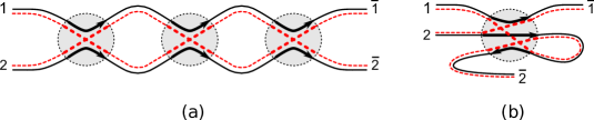
Figure 2. Two examples of semiclassical diagrams as drawn in the physics literature. These examples correspond to diagrams (d) and (e) of Fig. 4 in [47]

A semiclassical diagram is a schematic depiction of the topology of the $2n$-tuple $\{\gamma_{j},\gamma_{j}^{\prime}\}$. It describes which part of the trajectory $\gamma_{j}^{\prime}$ runs along which part of the trajectory $\gamma_{k}$ and what gets switched with what in the encounter region. Examples of diagrams typical in the physics literature are shown in Fig. 2. Note that to avoid clutter we often shorten labels $i_{j}$ to $j$ and labels $o_{j}$ to ${\overline{j}}$. In Fig. 2 the trajectories $\gamma_{1}$ and $\gamma_{2}$ running from $1$ to ${\overline{1}}$, and from $2$ to ${\overline{2}}$ correspondingly, are shown as solid black lines. The trajectories $\gamma^{\prime}$ are shown as dashed lines, while encounter regions are shown as shaded circles. In Fig. 2(a), the trajectory $\gamma_{1}^{\prime}$ (running from $2$ to ${\overline{1}}$) runs first along $\gamma_{2}$, then along $\gamma_{1}$, then $\gamma_{2}$ and finally $\gamma_{1}$ again. In Fig. 2(b), trajectory $\gamma_{2}^{\prime}$ starts from $1$ along $\gamma_{1}$, then follows $\gamma_{2}$ in the direction opposite to the direction of $\gamma_{2}$, finally switching to another part of $\gamma_{2}$, now in the same direction. This diagram requires TRS to contribute.

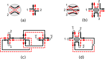
Figure 3. Untwisting the encounters into the vertices of the ribbon graph, (a) and (b). The ribbon graphs (c) and (d) correspond to the diagrams of Fig. 2. To read off the trajectories, we start at the open end labelled $1$ and follow the left side for $\gamma$ or the right side for $\gamma^{\prime}$. The leaves (vertices of degree 1) of the graph are shown as empty circles; the internal vertices are represented by the filled ellipses. Edges going to leaves are normally drawn short to save space. Other edges often have rectangular corners; the corners carry no particular meaning and were only employed due to the lack of artistic skill.

Starting with [6] and especially in [9], it was realized that “untwisting” the encounter region so that trajectories do not intersect (see Fig. 3), one obtains an equivalent picture but with a significant advantage: it is an object well studied in combinatorics and in some RMT literature, a (combinatorial) map. This term refers to a graph that is drawn on a surface without self-intersections. An important consequence of being drawn is that the ordering of edges around every vertex is fixed. If one traces a path along one side of an edge, upon arrival at a vertex there is a unique choice of the edge and the side along which to continue. This defines the boundary of the map. If the boundary is connected, the map is called unicellular. In-depth information about maps can be found, for example, in [29, 66]; the reader is referred to [75] for an especially accessible introduction with applications to RMT.

To highlight the boundary of a map, the edges are often thickened in a drawing (hence the alternative names “ribbon graph” or “fat graph”). This is the approach we take. The vertices of our maps are drawn as circles (or ellipses). Vertices of degree more than one are shaded, they correspond to the encounters. Vertices of degree one are unfilled, they are henceforth called leaves and correspond to the initial or final points of the trajectories. The edges of the map are shown as parallel curves connecting the vertices. The edges can have right angle turns in them (due to our lack of drawing skill) and Möbius-like twists. The latter are essential features of a map and indicate that the map can only be drawn on a non-orientable surface and the corresponding diagram requires TRS to contribute. The trajectories can now be read off as the sections of the boundary going from one leaf to another. As before, trajectories $\gamma_{j}$ are drawn in solid lines, while $\gamma_{j}^{\prime}$ are drawn dashed. The differences between unitary diagrams (with broken TRS) and orthogonal diagrams (contributing in the presence of TRS) and some other features are discussed after we introduce the principal diagrams in the next section.

3.2. Principal diagrams and untying

An example of a diagram which contributes to the third moment is depicted in Fig. 4(a). This diagram has two encounters that happen inside the cavity, and, according to the rules in Definition 1, its contribution is $(-N)^{2}/N^{7}$ (multiplied by $N_{1}^{3}N_{2}^{3}$ in the transmission case, once the summation over all possible incoming and outgoing channels is performed). However, there is a related diagram obtained by moving the first encounter close to the incoming lead, see Fig. 4(b). From geometric constraints, it follows that the channels $i_{1}$ and $i_{2}$ must coincide for this to be possible. According to Definition 1, this diagram has a different contribution. Indeed, the two edges leading to the encounter disappear and the encounter itself does not contribute anything. The resulting contribution is $N_{1}^{2}N_{2}^{3}(-N)/N^{5}$. Note the reduced power of $N_{1}$ due to the summation restricted by $i_{1}=i_{2}$. Importantly, when $N_{1}\sim N_{2}\sim N$, the overall order of the contribution does not change.

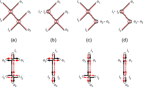
Figure 4. An example of a principal diagram and its untied versions contributing to the third moment.

Similarly, one can move the right encounter close to the outgoing lead, Fig. 4(c) or move both encounters, Fig. 4(d). The corresponding semiclassical contributions to the moment are $N_{1}^{3}N_{2}^{2}(-N)/N^{5}$ and $N_{1}^{2}N_{2}^{2}/N^{3}$. On the lower half of Fig. 4 the same diagrams are drawn as combinatorial maps. Note that in the map of Fig. 4(b) the lower vertex can be viewed as two vertices (each of degree one) shown on top of each other; the diagram then falls into two connected components. Thus an encounter happening in the lead is represented by “untying” the corresponding encounter in the diagram.

It is instructive to explore the parallels between the encounter happening in the lead (or untying a vertex in a diagram) with an expansion of the corresponding moment in random matrix theory.

Example 1.

Consider the RMT result for the second moment in the unitary case without TRS. We are going to use the general formula

(8) $$\langle U_{a_{1}a_{\overline{1}}}\ldots U_{a_{s}a_{\overline{s}}}U^{*}_{b_{1}b_{\overline{1}}}\ldots U^{*}_{b_{t}b_{\overline{t}}}\rangle_{\mathrm{CUE}(N)}=\delta_{t,s}\sum_{\sigma,\pi\in S_{t}}V^{\mathrm{U}}_{N}(\sigma^{-1}\pi)\prod_{k=1}^{t}\delta\!\left({a_{k}}-{b_{\sigma(k)}}\right)\,\delta\!\left({a_{\overline{k}}}-{b_{\overline{\pi(k)}}}\right),$$

where $S_{t}$ is the symmetric group of permutations of the set $\{1,\ldots,t\}$, $\delta_{k,n}=\delta(k-n)$ is the Kronecker delta (the latter notation is used solely to avoid nesting sub-indices) and the coefficient $V^{\mathrm{U}}_{N}(\sigma^{-1}\pi)$ depends only on the lengths of cycles in the cycle expansion of $\sigma^{-1}\pi$, i.e. on the conjugacy class of the permutation $\sigma^{-1}\pi$. This formula and the class coefficients $V^{\mathrm{U}}_{N}$ were first explored in detail by Samuel [60], although recently $V^{\mathrm{U}}_{N}$ became known as the “unitary Weingarten function” (after [71]).

Applying this formula to the second moment, setting $Z=S^{\mathrm{T}}$ we get

$$M_{2}(X) =\left\langle\sum_{\begin{subarray}{c}i_{1},i_{2}\cr o_{1},o_{2}\end{subarray}}Z_{i_{1},o_{1}}Z_{i_{2},o_{2}}Z^{*}_{i_{2},o_{1}}Z^{*}_{i_{1},o_{2}}\right\rangle$$

(9) $$=\sum_{\begin{subarray}{c}i_{1},i_{2}\cr o_{1},o_{2}\end{subarray}}\left[V^{\mathrm{U}}(\tau)+\delta_{i_{1},i_{2}}V^{\mathrm{U}}((1\,2)\tau)+\delta_{o_{1},o_{2}}V^{\mathrm{U}}(\tau(1\,2))+\delta_{i_{1},i_{2}}\delta_{o_{1},o_{2}}V^{\mathrm{U}}((1\,2)\tau(1\,2))\right]$$

(10) $$=N_{i}^{2}N_{o}^{2}V^{\mathrm{U}}(\tau)+N_{i}N_{o}^{2}V^{\mathrm{U}}((1\,2)\tau)+N_{i}^{2}N_{o}V^{\mathrm{U}}(\tau(1\,2))+N_{i}N_{o}V^{\mathrm{U}}((1\,2)\tau(1\,2)).$$

Here $N_{i}\times N_{o}$ is the size of the subblock $X^{\mathrm{T}}$ and $\tau=(1\,2)$ is called the principal target permutation, given by $\tau=\sigma^{-1}\pi$, where the permutations $\sigma=(1\,2)$ and $\pi=id$ map the first and last indices of $Z$ to the first and last indices of $Z^{*}$. This choice of $\sigma$ and $\pi$ is the only one available if the channels $i_{1}$, $i_{2}$ and $o_{1}$, $o_{2}$ are distinct. If $i_{1}=i_{2}$, there is an additional possibility $\sigma=id$ accounted for by the second term in (10) and so on.

The arguments of the functions $V^{\mathrm{U}}$ are formatted to highlight the connection to untying the diagrams. Multiplication of the permutation $\tau$ by $(1\,2)$ on the left corresponds to untying the ends $i_{1}$ and $i_{2}$ of a diagram. Multiplication by $(1\,2)$ on the right is the untying of the ends $o_{1}$ and $o_{2}$. This combinatorial encoding of untyings is explored in-depth in the Appendix. We remind the reader that we often shorten the leaf labels $i_{j}$ to $j$ and $o_{j}$ to ${\overline{j}}$.

We are now ready to present the mathematical definition of the principal diagram. Examples of unitary and orthogonal principal diagrams are shown in Figs. 3 and 5; the conditions entering the definitions are discussed at length in the first part of the paper [11]. When comparing Figs. 4 and 5 note the shortened leaf labels.

Definition 2.

The unitary principal diagram is a unicellular orientable map satisfying the following:

1. There are $t$ vertices of degree 1 (leaves) labelled with symbols $1,\ldots,t$ and $t$ leaves labelled with symbols ${\overline{1}},\ldots,{\overline{t}}$.

2. All other vertices have even degree greater than $2$.

3. A portion of the boundary running from one leaf to the next is called a boundary segment. Each leaf $j$ is incident to two boundary segments, one of which is a segment running to the leaf ${\overline{j}}$ and the other running to the leaf ${\overline{j-1}}$. The segments are given direction $j\to{\overline{j}}$ and $j\to{\overline{j-1}}$ and marked by solid and dashed lines correspondingly. The following conditions are satisfied:

   1. each part of the boundary is marked exactly once,

   2. each edge is marked solid on one side and dashed on the other, both running in the same direction.

Here unicellular means that the diagram has one face, i.e. its boundary is connected. We take the operation $j-1$ to be cyclic: $1-1=t$. The leaves labelled $1$, …, $t$ and ${\overline{1}}$, …, ${\overline{t}}$ we still call $i$-leaves and $o$-leaves correspondingly.

The conditions that make a valid orthogonal diagram are almost identical to the unitary case. The only significant difference is that trajectories $\gamma$ and $\gamma^{\prime}$ do not have to run in the same direction.

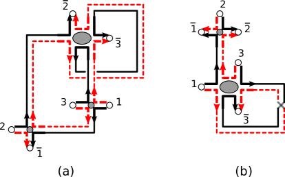
Figure 5. An example of a unitary and an orthogonal principal diagrams. The shaded circles (and ellipses) represent the vertices of even degrees (encounters).

Definition 3.

The orthogonal principal diagram is a locally orientable map satisfying the following:

1. There are $t$ leaves labelled with symbols $1,\ldots,t$ and $t$ leaves labelled with symbols ${\overline{1}},\ldots,{\overline{t}}$.

2. All other vertices have even degree greater than $2$.

3. Each leaf $j$ is incident to two boundary segments, one of which runs to the label ${\overline{j}}$ and is marked solid, and the other runs to ${\overline{j-1}}$ and is marked dashed. Each edge is marked solid on one side and dashed on the other.

If the two boundaries of an edge are marked as running in the same direction, this edge is called unitary, otherwise it is orthogonal. A unitary diagram has only unitary edges, while an orthogonal diagram can have either. A vertex is called unitary if all edges emanating from it are unitary. Note that if we perform a boundary walk of the diagram, the sides of a unitary edge will be traversed in opposite directions, while the orthogonal edge will be traversed in the same direction.

Finally, we formalize the notion of “untying” (it is explored in more detail in the Appendix).

Definition 4.

A vertex of even degree is called untieable (i.e. “can be untied”) if every second edge emanating from it leads directly to a leaf. If these leaves all have $i$-labels, the vertex is called $i$-untieable. If these leaves all have $o$-labels, the vertex is called $o$-untieable.

For example, the lower right vertex in Fig. 5(a) is $i$-untieable, while the upper vertex in Fig. 5(b) is $o$-untieable. It can also happen that every second edge leads to leaves with a mix of $i$- and $o$-labels, but only if the diagram is orthogonal (the lower vertex in Fig. 5(b) is an example).

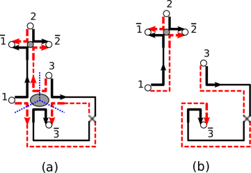
Figure 6. Untying a vertex of degree 3.

Having defined what an untieable vertex is, we explain the operation of untying, using the example of Fig. 6. An untieable vertex of degree $2m$ is untied by cutting it into $m$ parts, preserving the solid boundary segments. The dashed boundary segments are then reconnected as necessary. The semiclassical meaning of an untieable vertex is an encounter that can happen in a lead: because of the last rule in Definition 1, the contribution of a diagram with an encounter (vertex) happening in the lead is equal to the contribution of this diagram with the said vertex untied.

Our summation over semiclassical diagrams will be organized by grouping the contributions of a principal diagram together with its untied versions.

3.3. Contribution of a unitary diagram

By following the rules in Definition 1, the contribution of a principal diagram to the $n$-th moment $M_{n}(X)$ is given by $(-1)^{v}N_{i}^{n}N_{o}^{n}/N^{e-v}$, where $e$ is the number of edges of the diagram and $v$ the number of internal vertices. Again $N_{i}\times N_{o}$ is the size of $X^{\mathrm{T}}$. Having defined the untyings, we can now consider the contributions of the untied diagrams and for this we first return to Example 1.

Figure 7. Some diagrams contributing to the correlator in Example 2. The top row contains principal diagrams while untying their nodes leads to the diagrams below; see main text.

Example 2.

Similarly to equation (10), we reorganize the semiclassical contributions to the moment $M_{2}(X)$ as

(11) $$M_{2}(X)=N_{i}^{2}N_{o}^{2}D^{\mathrm{U}}(\tau)+N_{i}N_{o}^{2}D^{\mathrm{U}}((1\,2)\tau)+N_{i}^{2}N_{o}D^{\mathrm{U}}(\tau(1\,2))+N_{i}N_{o}D^{\mathrm{U}}((1\,2)\tau(1\,2)),$$

where $D^{U}(\tau)$ is the contribution of all unitary principal diagrams, $D^{U}((1\,2)\tau)$ is the contribution of the principal diagrams after untying a vertex with leaf labels $i_{1}$ and $i_{2}$ and so on. In Figure 7 we have several diagrams contributing to the sum. They are arranged in the following manner. The four rows list diagrams contributing to the terms $D^{\mathrm{U}}(\tau)$, $D^{\mathrm{U}}((1\,2)\tau)$, $D^{\mathrm{U}}(\tau(1\,2))$ and $D^{\mathrm{U}}((1\,2)\tau(1\,2))$ correspondingly (top to bottom). The diagrams in the lower three rows are the results of untying the diagram in the top row. For example, the diagrams in the second row are the result of $i$-untying the diagram above it and are accounted for in the term $D^{\mathrm{U}}((1\,2)\tau)$. Similarly, the diagrams in the third row are the result of $o$-untying the top diagram and contribute to $D^{U}(\tau(1\,2))$. For the final row we $i$-untie one vertex and $o$-untie the other. Some untyings are not possible and the corresponding positions are left empty.

Note that we are essentially using $\tau$ as a placeholder symbol with the meaning “principal diagram”. If one chooses to delve deeper into the combinatorics of semiclassical diagrams (as done in [11] and the Appendix), $\tau$ takes the meaning of the target permutation. For unitary principal diagrams, $\tau=(1\ 2\ \ldots\ t)$ and the operation of untying corresponds to the actual multiplication of permutations. This is explored in detail in the Appendix.

We now observe that the contributions of all diagrams in a given column are of the same order (taking the prefactors in (11) into consideration). For example the contributions of the last column are

$$-\frac{N_{i}^{2}N_{o}^{2}}{N^{5}}+\frac{N_{i}N_{o}^{2}}{N^{4}}+\frac{N_{i}^{2}N_{o}}{N^{4}}-\frac{N_{i}N_{o}}{N^{3}}.$$

Example 3.

The diagram of Figure 5(a) and its untied version give the contribution

(12) $$-\frac{N_{i}^{3}N_{o}^{3}}{N^{7}}+\frac{N_{i}^{2}N_{o}^{3}}{N^{6}}.$$

Note that we only untie the vertices that are “untieable” in the original diagram. For example, the lower left vertex of this diagram becomes untieable after untying the lower right vertex, but it is not a part of this particular sum.

To summarize, if a $2m$-vertex of a unitary diagram becomes untied, its contribution is missing one vertex factor of $(-N)$, $m$ edge factors of $1/N$ and there is only one factor of $N_{j}$ where before there were $m$. To include the contribution of the untied diagrams with the principal diagram, we multiply the contribution of the principal diagram by the factor

(13) $$\left(1-\frac{N^{m-1}}{N_{j}^{m-1}}\right),$$

for each $2m$ vertex which can be untied, where $N_{j}$ depends on whether the vertex is $i$- or $o$-untied and is simply the number of channels in the corresponding lead.

Carrying on Example 3, we then have

Example 4.

The diagram of Figure 5(a) and its untied version together give the contribution

$$-\frac{N_{i}^{3}N_{o}^{3}}{N^{7}}\left(1-\frac{N}{N_{i}}\right),$$

which is (12).

We also mention that the contributions listed above are valid both for the transmission moments, where $X$ is the off-diagonal matrix ${\boldsymbol{t}}$ in (1) [with $N_{i}=N_{1}$ and $N_{o}=N_{2}$], and for the reflection moments (where $X$ is the diagonal matrix ${\boldsymbol{r}}$). In the latter case we additionally have $N_{i}=N_{o}=N_{1}$.

3.4. Contribution of an orthogonal diagram

The situation is somewhat different in the orthogonal case. If the vertex is purely $i$- or $o$-untieable, the contribution adjustment is exactly the same as in the unitary case. However, if the leaf labels involve a mixture of labels of the two types, then the corresponding Kronecker delta [see Equation (9)] mixes $i$ and $o$ indices. For transmission moments, where the incoming and outgoing channels are in separate leads, those cannot possibly coincide and the corresponding untying produces 0 additional contribution. When calculating reflection moments, such “mixed” untieable vertices do contribute and their contribution is calculated according to the rules above (with the understanding that $N_{i}=N_{o}$). Namely, the contribution of the untied diagram is divided by $-N_{i}^{m-1}/N^{m-1}$.

Example 5.

Consider the diagram of Fig. 5(b). The top vertex is $o$-untieable (if $o_{1}$ and $o_{2}$ are the same channel), while untying the lower vertex requires that $i_{1}$, $i_{3}$ and $o_{3}$ be the same channel and therefore in the same lead. This is possible only in the input and output leads coincide, i.e. we are considering a reflection quantity. The total contribution of this diagram, viewed as the principal diagram, is

$$\frac{N_{1}^{3}N_{2}^{3}}{N^{6}}\left(1-\frac{N}{N_{2}}\right),$$

to the (third) transmission moment and

$$\frac{N_{1}^{6}}{N^{6}}\left(1-\frac{N}{N_{1}}\right)\left(1-\frac{N^{2}}{N_{1}^{2}}\right),$$

to the reflection moment.

4. From principal diagrams to base structures

Having understood how to evaluate the contribution of a particular principal diagram and its untied version, we now turn to the question of generating the diagrams. Our aim eventually is to evaluate $M_{n}$ for any $n$, but only to several leading orders of $1/N$, assuming $N_{1}\sim N_{2}\sim N$.

As mentioned in Section 3.3, the contribution of a principal diagram to the $n$-th moment is $(-1)^{v}N_{i}^{n}N_{o}^{n}/N^{e-v}$, where $e$ and $v$ are the number of edges and internal vertices of the diagram respectively. Denoting the total number of vertices (including the leaves) by ${\widetilde{v}}$ and noting that ${\widetilde{v}}=v+2n$, we see that the order of the contribution is $1/N$ to the power $e-{\widetilde{v}}$. The untyings of the principal diagram contribute at the same order.

Since the target permutation of the principal diagram is (see Remark 2 in the Appendix) the palindromic grand cycle $\tau=(1\,2\ldots n)({\overline{n}}\ldots{\overline{2}}\,{\overline{1}})$, the boundary is connected and the diagrams are unicellular (i.e. have one face). The genus of an orientable map is defined as the smallest genus of a surface on which the map can be drawn without self-intersection. Recalling that the genus $g$ of unicellular orientable maps can be found as

(14) $$2g=1+e-{\widetilde{v}},$$

the order of a diagram’s contribution is $1/N$ to the power $2g-1$. An asymptotic expansion in $1/N$ is then a type of genus expansion, familiar from Gaussian ensembles and their applications [75]. The genus of an orientable map must be integer, however, if we take equation (14) as the definition in the non-orientable case, orthogonal maps can have half-integer “genus” (there is a notion of demigenus for non-orientable surfaces, which is an integer and coincides with our value $2g$).

Our task is complicated by the fact that we would like to obtain moments of arbitrary order $n$. Thus our typical diagram has a low genus and many vertices. This suggests that we can enumerate the eligible diagrams by planting trees (which provide many vertices at no cost to genus) onto base structures that have the required genus.

Definition 5.

A base structure is a unicellular map with no vertices of degree 1 or 2 and with a labelled “starting” edge-side and specified direction.

It is easy to see that the number of possible base structures contributing at a given order is finite. Indeed, since the minimal vertex degree is 3, the number of edges can be estimated as $e>3{\widetilde{v}}/2$ and therefore, from (14), the number of vertices is bounded by $2(2g-1)$.

Remark 1.

Another name for base structures in the literature is “schemes”, see [22, 21].

In the sections that follow we describe the algebraic procedures for generating the base structures and planting trees. Before we do so, we present several examples that illustrate the main ideas which we develop further in Section 5.

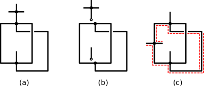
Figure 8. (a) An example of a diagram appearing in Fig. 7 and (b) its decomposition into a base structure and (rooted) trees. (c) An example of invalid diagram and an attempt to label its boundary segments (only dashed boundary segments are shown): some edges will be labelled the same on both sides violating one of the requirements of Definition 2.

Fig. 8(a)-(b) shows an example of a diagram, its base structures and the trees. Reversing the process, we will plant trees with internal vertices of even degrees greater than 2. Obviously we have to plant enough trees to make all vertices on the base structure have even degree. However, as the example of Fig. 8(c) shows, this is not sufficient to generate a valid diagram. The obstacle is the requirement that the solid and dashed trajectories match along the boundary to satisfy Definitions 2 or 3. It is possible to theoretically characterize a map whose boundaries can be properly labelled solid and dashed as required. Rather than doing this, however, we will describe a construction method which generates only valid diagrams.

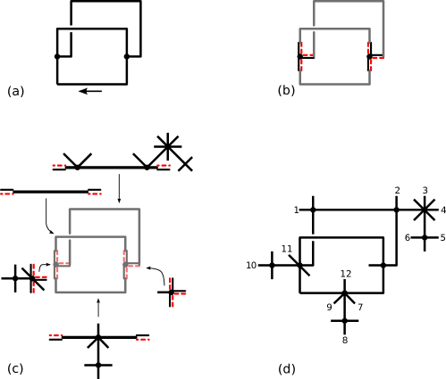
Figure 9. (a) The base structure, (b) pre-marking the edge-ends, (c) planting trees on vertices and edges, (d) labeling the leafs. To avoid clutter only the leaf labels without bars are shown.

We first outline the method using the example of Fig. 9. Starting with a base structure (details in section 4.1) we pre-label the stubs of edges around every vertex with dashed and solid lines. By a “stub” of an edge we understand a small part of edge attached to the vertex. The pre-labeling can be done in arbitrary manner, provided the lines are different on the two sides of each edge, see Fig. 9(b). Then we plant rooted trees (section 5.1) on edges and vertices. The parity of the number of trees and their type is fully determined by the pre-marking (sections 5.2 and 5.3). The contribution of the pre-marked diagram to the total sum is expressible as the product of the contributions of its constituent parts: edges and vertices. Finally, we will sum the contributions over all possible pre-markings.

4.1. Generating base structures

The semiclassical diagrams are drawn as ribbon graphs with the edges fattened to have two sides. We now present a combinatorial description of the base structures which is a slightly modified version of Tutte’s axiomatization [29, 66].

From the definition of the base structure, we obtain the canonical boundary walk which starts at the marked edge in the marked direction and passes every edge twice (once on each side). As we go along the boundary, we label the edge-sides with numbers $1,\ldots 2m$, where $m$ is the number of edges in the base structure. We also mark the direction of each edge-side. The reversal of an edge-side (i.e. the same edge-side running in the opposite direction) is denoted by the same symbol with a bar. Therefore the reversal of the canonical boundary walk passes the edge-sides ${\overline{2m}},\ldots{\overline{1}}$. It turns out that a base structure with such labelling is uniquely specified by the pairing (matching) of the labels on the opposite sides of the edges.

To generate base structures with $m$ edges, we consider permutations on the set

$$Z_{2m}=\{1,\ldots,2m,{\overline{2m}},\ldots,{\overline{1}}\},$$

of $4m$ elements. The permutation

(15) $$T=(1\,{\overline{1}})(2\,{\overline{2}})\cdots(2m\,{\overline{2m}}),$$

encodes the operation of reversal while the face permutation

(16) $$\phi=(1\,2\ldots 2m)({\overline{2m}}\ldots{\overline{2}}\,{\overline{1}}),$$

corresponds to the canonical boundary walk of the unique face of the map and its reversal. With these pieces of data fixed, the unicellular map is described by one permutation.

Definition 6.

A unicellular map in canonical form is a permutation $\varepsilon$ that

• is a fixed-point free involution (i.e. has only cycles of length 2),

• has no cycles of the form $(x\,{\overline{x}})$,

• commutes with $T$: $T\varepsilon=\varepsilon T$.

The cycles of $\varepsilon$ correspond to the matching of different sides of the edges. For example, a cycle of $(1\ 3)$ means that one edge has sides numbered $1$ and $3$ running in the opposite directions. Then, the reversals ${\overline{1}}$ and ${\overline{3}}$ must also be matched. This is ensured by the commutativity requirement: $T(1\ 3)T^{-1}=({\overline{3}}\,{\overline{1}})$.

The cycle of the form $(1\,{\overline{3}})$ [and its counterpart $(3\,{\overline{1}})$] would denote an edge with sides $1$ and $3$ running in the same direction. There are no such edges in an orientable map. An edge of the form $(j\,k)({\overline{k}}\,{\overline{j}})$ we will call a unitary edge, while the edge of the form $(j\,{\overline{k}})(k\,{\overline{j}})$ will be referred to as an orthogonal edge. We stress that a diagram contributing to an orthogonal (i.e. with TRS) quantity may contain some unitary edges. It may even contain only unitary edges: a unitary diagram contributes in both cases.

The permutation

(17) $$\nu=\phi\varepsilon,$$

is called the vertex permutation. Each vertex of the map corresponds to two cycles that list the edge-sides leaving the vertex. One cycle has the edge-sides that keep their edge to their left, listed anticlockwise around the vertex. The other lists the edge-sides that keep their edges to their right, in the clockwise order around the vertex. Naturally, the base diagrams are unicellular maps whose vertex permutation only has cycles of length 3 or higher.

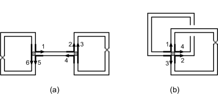
Figure 10. Two examples of orthogonal base diagrams. The diagram in (a) has one unitary edge (in the middle) and two orthogonal edges. The diagram in (b) has one orthogonal edge (left) and one unitary edge (right). Note that the presence of a twist in the edge does not mean the edge is orthogonal.

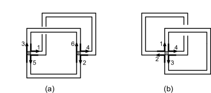
Figure 11. Two examples of unitary base diagrams. These are the only unitary diagrams of genus $1$.

Example 6.

The map from Fig. 10(a) can be represented as

$$\varepsilon=(1\,4)(2\,{\overline{3}})(5\,{\overline{6}})({\overline{5}}\,6)({\overline{2}}\,3)({\overline{1}}\,{\overline{4}}),\quad\mbox{with}\quad\nu=(1\,5\,{\overline{5}})({\overline{4}}\,{\overline{6}}\,6)(2\,{\overline{2}}\,4)({\overline{1}}\,{\overline{3}}\,3),$$

while the map of Fig. 10(b) can be written as

$$\varepsilon=(1\,3)(2\,{\overline{4}})({\overline{2}}\,4)({\overline{1}}\,{\overline{3}}),\quad\mbox{with}\quad\nu=(1\,4\,{\overline{1}}\,{\overline{2}})(2\,{\overline{3}}\,{\overline{4}}\,3).$$

When performing a computation, we choose a canonical way to order the cycles in the permutation $\varepsilon$. For example, we order the elements of $Z_{2m}$ by mapping ${\overline{x}}$ to $x+2m$ for all $x\in\{1,\ldots,2m\}$ and order the cycles in a palindromic fashion

$$\varepsilon=(s_{1}\,r_{1})\,(s_{2}\,r_{2})\cdots(s_{v}\,r_{v})({\overline{s_{v}}}\,{\overline{r_{v}}})\cdots({\overline{s_{2}}}\,{\overline{r_{2}}})\,({\overline{s_{1}}}\,{\overline{r_{1}}}),$$

with the ordering conditions

$$s_{j}<r_{j},\quad s_{j}<{\overline{s_{j}}},\quad s_{j}<{\overline{r_{j}}},\quad s_{j}\leq s_{j+1}.$$

With the additional requirement $r_{j}\neq{\overline{s_{j}}}$ the above palindromic permutations automatically satisfy all the conditions of Definition 6. Calculating the permutation $\nu$ we establish how the edges are connected to the vertices. At this point we exclude the diagrams that have cycles of length 1 or 2 in the permutation $\nu$. Next we calculate the semiclassical contribution of the base structure following the prescriptions explained in Section 5.

With broken TRS, all the edges must be traversed on both sides by semiclassical trajectories travelling in the same direction. Or, equivalently,

Definition 7.

A unitary base structure is an orientable base structure.

The cycles of $\varepsilon$ can then only involve pairs of labels either both with bars or both without bars. Removing the redundant half of $\varepsilon$ involving bars, we return to the standard definition:

Definition 8.

An orientable map of size $m$ is a triple $({\widetilde{\varepsilon}},{\widetilde{\nu}},{\widetilde{\phi}})$ of permutations of size $2m$ such that all cycles of ${\widetilde{\varepsilon}}$ have length 2 and ${\widetilde{\nu}}{\widetilde{\varepsilon}}={\widetilde{\phi}}$.

For the unitary base structures we have ${\widetilde{\phi}}=(1\,2\ldots 2m)$ and we again exclude diagrams with vertices of degree 1 and 2.

Example 7.

The maps from Fig. 11 can be represented as

$${\widetilde{\varepsilon}}=(1\,4)(2\,5)(3\,6),\quad\mbox{with}\quad{\widetilde{\nu}}=(1\,5\,3)(2\,6\,4),$$

and

$${\widetilde{\varepsilon}}=(1\,3)(2\,4),\quad\mbox{with}\quad{\widetilde{\nu}}=(1\,4\,3\,2),$$

where the vertices can be read off clockwise in Fig. 11.

As the size of the permutations is halved, the search for unitary base structure is computationally more efficient than the search for the orthogonal ones. This allows us to go to a higher genus (semiclassical correction order) in the case of broken TRS. However, if, for a given genus, the orthogonal base structures have already been found, the unitary structures can be efficiently selected as a subset of those. In Table 1 we list all orthogonal base structures of genus $1$; the unitary base structures are those whose permutation contains no bars, which were sketched in Fig. 11.

$m$	$\varepsilon$	$m$	$\varepsilon$
$2$	$(1\,3)(2\,4)$	$3$	$(1\,4)(2\,5)(3\,6)$
	$(1\,{\overline{2}})(3,{\overline{4}})$		$(1\,{\overline{2}})(3\,6)(4\,{\overline{5}})$
	$(1\,3)(2,{\overline{4}})$		$(1\,{\overline{3}})(2\,5)(4\,{\overline{6}})$
	$(1\,{\overline{3}})(2,4)$		$(1\,4)(2\,{\overline{3}})(5\,{\overline{6}})$
	$(1\,{\overline{4}})(2,{\overline{3}})$		$(1\,4)(2\,{\overline{6}})(3\,{\overline{5}})$
			$(1\,{\overline{5}})(2\,{\overline{4}})(3\,6)$
			$(1\,{\overline{6}})(2\,5)(3\,{\overline{4}})$

Table 1. Base structures of genus $g=1$ with $m$ edges. Only half of the palindromic representation of $\varepsilon$ is given.

To illustrate the difficulty of summation over the base structures, in Table 2 we list the number of the base structures of given genus $g$ and number of edges $m$. In the unitary (orientable) case these numbers have been studied, in particular, in [25]. In the orthogonal (locally orientable) case, related quantities have been considered in [12].

$g$	$m$	orth.	unit.	$g$	$m$	orth.	unit.
1	2	5	1	2	4	509	21
	3	7	1		5	4508	168
3/2	3	41			6	14235	483
	4	198			7	20867	651
	5	285			8	14516	420
	6	128			9	3885	105

Table 2. Number of base structures at a given genus $g$ with $m$ edges.

5. Summation over principal diagrams

Given a base structure we will now graft trees onto its edges and vertices to create the principal diagrams.

5.1. Trees

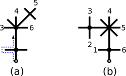
Figure 12. Examples of trees: (a) an $o$-tree and (b) an $i$-tree. The root is marked by the empty circle. Only the $i$-leaves are labelled to avoid clutter. A beginning of the boundary walk is shown by the dotted line. In example (a), the leaf number 1 is located on some other part of the diagram, prior to the place where the tree is rooted.

The leaves of grafted trees correspond to the incoming channels (with labels from the set $\{1,2,\ldots,n\}$) and outgoing channels (with labels from $\{{\overline{1}},{\overline{2}},\ldots,{\overline{n}}\}$). For simplicity we will refer to the incoming channel leaves as $i$-leaves and the outgoing leaves as $o$-leaves. The boundary walk of the trees alternatively visits $i$ and $o$-leaves. There is an even number of leaves altogether, but the root leaf (which is where the tree is to be attached to the base structure) is not labeled. Thus an odd number of leaves is labelled. The trees with more $o$-leaves than $i$-leaves will be called $o$-trees; their semiclassical contribution will be denoted by $f$. The contribution of the trees with more $i$-leaves (“$i$-trees”) will be denoted $\hat{f}$. The exact form of the contribution depends on the particular transport quantity that is being considered and will be derived in sections 6.2 and 6.7.

We mention that such rooted trees have also been used to find the leading order moment generating functions for the transmission eigenvalues [6] and the Wigner delay times [8].

5.2. Edges

We now derive the contribution of an edge of a base structure on which some trees have been grafted. When trees are grafted at a point on the edge, the point becomes a vertex. To form a vertex of even degree an even number of trees must be grafted. The trees can be placed on either side of the edge which creates two types of vertices: odd vertices with an odd number of trees attached to either side (for example, the vertex on the lower edge of Fig. 9), and even vertices with an even number of trees on either side (both vertices on the upper edge of Fig. 9).

The semiclassical contribution of a vertex depends on $f$ and $\hat{f}$ as well as the exact transport quantity considered. For now, we denote by $A$ the contribution of an even node. The odd nodes come in three further subvarieties: those with a majority of $o$-trees attached, those with a majority of $i$-trees and those with an equal number. This last possibility occurs if and only if the edge is orthogonal (i.e. traversed in the same direction by the boundary walk of the base structure). Their contributions will be denoted by $B_{o}$, $B_{i}$ and just $B$ correspondingly.

After pre-marking of the edge ends with dashed and solid lines, 8 types of edge arise. These depend on the pre-marking of the ends (two types for each end) and on whether the edge is unitary or orthogonal. Examples of these types are given in Fig. 13.

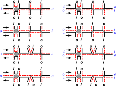
Figure 13. Examples of all possible types of pre-labelled edges. The unitary edges are shown on the left, orthogonal are shown on the right (the direction of the boundary walk is indicated by arrows).

We distinguish the different types using the labels that would be assigned to the edge ends. This label depends on the direction of the boundary walk along the edge: a boundary segment starts at $i$ and ends at $o$, see Fig. 14. It is important to note that a solid segment runs along the boundary walk, while the dashed one runs in the opposite direction. Implementing the above rule results in having one label per end for a unitary edge but two labels per edge end for an orthogonal edge: one for each side.

Assigning the labels to the edge ends also preserves the alternation of the $o$ and $i$ trees around the edge structure. The edges on the left side of Fig. 13 give contributions $E_{\mathrm{u}}(i,o)$, $E_{\mathrm{u}}(o,i)$, $E_{\mathrm{u}}(i,i)$, $E_{\mathrm{u}}(o,o)$ listed top to bottom. The contributions $E_{\mathrm{u}}(i,o)$ and $E_{\mathrm{u}}(o,i)$ are equal, since their configurations are related by the rotation by $\pi$.

The contributions of orthogonal edges is denoted by reading the edge-end labels in the clockwise direction around the edge: $E_{\mathrm{o}}(oi,oi)$, $E_{\mathrm{o}}(io,io)$, $E_{\mathrm{o}}(oi,io)$ and $E_{\mathrm{o}}(io,oi)$ for the edges on the right side of Fig. 13 listed top to bottom. There are only two distinct contributions: two pairs are related by top-bottom reflection, resulting in $E_{\mathrm{o}}(oi,oi)=E_{\mathrm{o}}(io,io)$ and $E_{\mathrm{o}}(oi,io)=E_{\mathrm{o}}(io,oi)$.

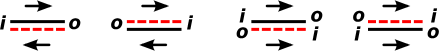
Figure 14. Rules for labeling edge ends: $i$ at the start of a solid segment or the end of a dashed segment; $o$ at the end of a solid or the start of a dashed segment.

We will now derive the contributions of a unitary edge in terms of the already defined quantities. The structure of every edge is a sequence of alternating odd nodes $B_{o}$ and $B_{i}$, separated by blocks of even nodes, see Fig. 15. Each block can have any number of even nodes (or none at all), giving the contribution

$$y+y^{2}A+y^{3}A^{2}+\ldots=\frac{y}{1-yA},$$

where $y$ is the semiclassical contribution of an edge in the diagram (not to be confused with the “composite” edge of the base structure). From Definition 1, $y=1/N$ for the quantities we consider in section 6, though it differs in other physical situations.

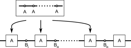
Figure 15. The structure of the edge $E_{\mathrm{u}}(o,i)$: odd nodes separated by sequences of even nodes.

The edge types $E_{\mathrm{u}}(o,i)$ and $E_{\mathrm{u}}(i,o)$ contain an equal number of odd vertices $B_{o}$ and $B_{i}$, leading to

(18) $$E_{\mathrm{u}}(o,i)=E_{\mathrm{u}}(i,o)=\sum_{n=0}^{\infty}\frac{B_{o}^{n}B_{i}^{n}y^{2n+1}}{(1-yA)^{2n+1}}=\frac{y(1-yA)}{(1-yA)^{2}-y^{2}B_{o}B_{i}}$$

The $E_{\mathrm{u}}(o,o)$ edge has an extra odd $B_{i}$ vertex (and an extra string of even nodes) and we have

(19) $$E_{\mathrm{u}}(o,o)=\frac{yB_{i}}{(1-yA)}E_{\mathrm{u}}(o,i)=\frac{y^{2}B_{i}}{(1-yA)^{2}-y^{2}B_{o}B_{i}}.$$

Similarly,

(20) $$E_{\mathrm{u}}(i,i)=\frac{y^{2}B_{o}}{(1-yA)^{2}-y^{2}B_{o}B_{i}}.$$

For the orthogonal edges, the difference with respect to unitary edges is that the odd nodes are all of the same type with contribution $B$. The edge $E_{\mathrm{o}}(oi,oi)$ has an even number of $B$ vertices, while $E_{\mathrm{o}}(oi,io)$ has an odd number, leading to

(21) $$E_{\mathrm{o}}(oi,oi)=E_{\mathrm{o}}(io,io)=\frac{y(1-yA)}{(1-yA)^{2}-y^{2}B^{2}},\qquad E_{\mathrm{o}}(oi,io)=E_{\mathrm{o}}(io,oi)=\frac{y^{2}B}{(1-yA)^{2}-y^{2}B^{2}}.$$

We remark that for the transport quantities we consider it turns out that $B_{i}B_{o}=B^{2}$ which greatly simplifies the calculations.

5.3. Vertices

Finally we can also graft trees onto the vertices of the base diagram. After the edge stubs of the base diagram have been pre-labelled, we can assign labels to the edge stubs adjacent to a given vertex according to the rules summarized in Fig. 14. Knowing the labels we determine what type of trees can be planted in the sectors between the existing edges. There are three possibilities: between labels $i$ and $i$ one has to plant an odd number of trees, majority of them of type $o$; between labels $o$ and $o$ one plants an odd number of trees, majority of them type $i$; between labels $i$ and $o$ one plants an equal number of $i$ and $o$ trees. The resulting sectors will be referred to as $o$-odd, $i$-odd and even correspondingly, see Fig. 16.

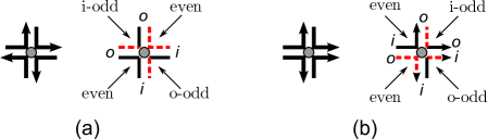
Figure 16. Examples of pre-labelled vertices, (a) unitary and (b) orthogonal. The types of resulting sectors are indicated.

The contribution of an even sector is thus

$$1+f\hat{f}+\left(f\hat{f}\right)^{2}+\ldots=\frac{1}{1-f\hat{f}},$$

while the $o$ and $i$-odd sectors contribute

$$\frac{f}{1-f\hat{f}}\qquad\mbox{and}\qquad\frac{\hat{f}}{1-f\hat{f}},$$

correspondingly.

Recording the labels of the edge stubs clockwise around a base diagram vertex of degree $k$, we obtain the sequence $(b_{1},\ldots,b_{k})$. The semiclassical contribution of that vertex $V_{k}(b_{1},\ldots,b_{k})$ then depends on the number of times $o$ follows $o$ (denoted by $p$) and the number of time $i$ follows $i$ (denoted by $q$) in that sequence (considered cyclically). For example the code for the vertex in Fig. 16(b) is $oi,i,oi,o$ with $p=1$ and $q=1$.

Finally, a special correction factor may arise due to the vertex becoming untieable (see Definition 10). Since only the planted trees can lead directly to a leaf, it is clear that the vertex can only become untieable if all sectors are odd. In addition (when calculating the transmission moments), all sectors must have the same type. However, it is easy to see that the sectors on the two sides of an orthogonal edge always have different type (if both odd). Therefore, in the calculation of the transmission moments, the untying of orthogonal vertices does not contribute (see section 3.4). In the calculation of reflection moments the type restriction becomes irrelevant and a vertex should receive a correction factor whenever all sectors are odd.

To summarize, denoting the semiclassical contribution of the vertex (of the final diagram) by $x$ and the untieable factor by $\chi$ (to be calculated later), the contribution of a vertex is

$$V_{k}(b_{1},\ldots,b_{k})=x\frac{f^{q}\hat{f}^{p}}{(1-f\hat{f})^{k}}\chi.$$

5.4. The algorithm

The contributions of edges and vertices are multiplicative: for a given labelling of the edge stubs, we determine the contribution of each constituent part of the base structure and multiply them together to obtain the contribution of the pre-labelled base structure itself. To obtain the total contribution of the base structure we sum over all possible pre-labellings.

In practical implementation, it is more convenient to assign the symbols $i$ or $o$ to the ends of a unitary edge and symbols $io$ or $oi$ to the ends of an orthogonal edge and then assign the opposite values to the corresponding stubs of the vertices. The unitary diagrams are a subclass of the orthogonal ones, so we will concentrate on the orthogonal case.

We will now describe the formal algorithm. For a diagram with $m$ edges, introduce $4m$ variables $b_{1},\ldots,b_{2m},b_{{\overline{1}}},\ldots,b_{{\overline{2m}}}$. These will take values in the set $\{i,o,io,oi\}$. We introduce two operations on this set, given by

(22) $${\widetilde{i}} =o, {\widetilde{o}} =i, {\widetilde{io}} =oi, {\widetilde{oi}} =io,$$

(23) $${\widehat{i}} =i, {\widehat{o}} =o, {\widehat{io}} =oi, {\widehat{oi}} =io.$$

We remind the reader that the base diagram is encoded by the permutation $\varepsilon$ (which describes the edges) and the derived permutation $\nu$ (which describes vertices). Each edge (or vertex) is equivalently described by two cycles of the permutation $\varepsilon$ (or $\nu$). In the algorithm we use only one of these cycles; it does not matter which one is used.

We go through all possible assignments of values to the variables $b_{z}$ such that the following conditions are satisfied:

1. if $(z_{1}\,z_{2})$ is a unitary edge then $b_{z_{1}}\in\{i,o\}$, otherwise $b_{z_{1}}\in\{io,oi\}$.

2. the variables on the opposite sides of an edge end are related by

   (24) $$b_{z}={\widehat{b}}_{{\overline{\varepsilon(z)}}}.$$

Then, every cycle $(z_{1}\,z_{2})$ in (the first half of) the permutation $\varepsilon$ gives rise to the factor $E(b_{z_{1}},b_{z_{2}})$. Every cycle $(z_{1}\,z_{2}\,\ldots z_{k})$ in (half of) the permutation $\nu$ contributes the factor $V_{k}({\widetilde{b_{z_{1}}}},{\widetilde{b_{z_{2}}}},\ldots,{\widetilde{b_{z_{k}}}})$.

Example 8.

Consider the map from Fig. 10(a) in Example 6. The labels of the variables $b_{z}$ are shown in Fig. 17(a). An example assignment of the edge end, illustrated in Fig. 17(b), is

$$b_{1}=i,\quad b_{4}=o,\quad b_{5}=io,\quad b_{{\overline{5}}}=oi,\quad b_{2}=io,\quad b_{{\overline{2}}}=io,$$

with the other variables deduced using (24):

$$b_{3}={\widehat{b}}_{{\overline{{\overline{2}}}}}=oi,\quad b_{{\overline{4}}}={\widehat{b}}_{{\overline{{\overline{1}}}}}=i,\quad b_{6}=oi,\quad b_{{\overline{1}}}=o,\quad b_{{\overline{3}}}=oi,\quad b_{{\overline{6}}}=io.$$

Note that the edge stubs of the vertices get the opposite values. Altogether, the contribution of this assignment is

$$E_{\mathrm{u}}(i,o)V_{3}(oi,oi,i)E_{\mathrm{o}}(io,oi)V_{3}(o,oi,io)E_{\mathrm{o}}(io,io).$$

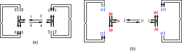
Figure 17. Edge variable labels and a possible assignment of the variables.

The total contribution of this base diagram is

$$\sum_{\begin{subarray}{c}b_{1},b_{4}\in\{i,o\}\\ b_{2},b_{{\overline{3}}},b_{5},b_{{\overline{6}}}\in\{io,oi\}\end{subarray}}E_{\mathrm{u}}(b_{1},b_{4})V_{3}({\widetilde{b_{2}}},{\widetilde{b_{{\overline{2}}}}},{\widetilde{b_{4}}})E_{\mathrm{o}}(b_{2},b_{{\overline{3}}})V_{3}({\widetilde{b_{1}}},{\widetilde{b_{5}}},{\widetilde{b_{{\overline{5}}}}})E_{\mathrm{o}}(b_{5},b_{{\overline{6}}}),\qquad b_{{\overline{5}}}={\widetilde{b_{{\overline{6}}}}},\ b_{{\overline{2}}}={\widetilde{b_{{\overline{3}}}}}.$$

Similarly, the contribution of the base diagram of Fig. 10(b) is

$$\sum_{\begin{subarray}{c}b_{1},b_{3}\in\{i,o\}\\ b_{2},b_{{\overline{4}}}\in\{io,oi\}\end{subarray}}E_{\mathrm{u}}(b_{1},b_{3})V_{4}({\widetilde{b_{1}}},{\widetilde{b_{4}}},{\widetilde{b_{{\overline{1}}}}},{\widetilde{b_{{\overline{2}}}}})E_{\mathrm{o}}(b_{2},b_{{\overline{4}}}),\qquad b_{4}={\widetilde{b_{2}}},\ b_{{\overline{1}}}=b_{3}.$$

As we start with a base structure with a marked half-edge and end up with the diagram with a marked leaf, we need to account for all the possibilities to unmark the edge and mark a leaf. The contribution of a diagram will be multiplied by $n/(2m)$, where $m$ is the number of edges in the base diagram and $2n$ is the number of leaves in the complete diagram. Note that our system of pre-labelling determines which leaves are $i$ and which are $o$, so there are only $n$ possibilities to choose the leaf $i_{1}$. Since we are dealing with generating functions with respect to $n$, the factor of $n$ will be obtained by applying the operator

(25) $$s\frac{d}{ds}$$

to the generating function of the variable $s$.

To summarize, we have sketched an algorithm to calculate the contribution of all diagrams of a given order. For a given order, the number of base structures is finite. We enumerate all of them, then enumerate all possible leaf-markings of their edge-ends. For each leaf-marking we multiply together the contributions of all edges and vertices.

6. Moment generating functions

With the organisation of semiclassical diagrams in terms of principal diagrams and their untied versions and the algorithmic approach to generate and evaluate such diagrams, we can now proceed to evaluate moment generating functions for various transport quantities.

6.1. Moments of the transmission eigenvalues

Here we consider the typical transport problem of the linear moments of the transmission eigenvalues of the matrix ${\boldsymbol{t}}^{\dagger}{\boldsymbol{t}}$ based on the transmitting subblock of the scattering matrix (1) which connects the $N_{1}$ channels in one lead to the $N_{2}$ channels in the other. We will obtain an expansion of the moment generating function

(26) $$T(s)=\sum_{n=1}s^{n}\left\langle\operatorname{Tr}\left[{\boldsymbol{t}}^{\dagger}{\boldsymbol{t}}\right]^{n}\right\rangle=NT_{0}(s)+T_{1}(s)+N^{-1}T_{2}(s)+N^{-2}T_{3}(s)+N^{-3}T_{4}(s)+\ldots$$

in inverse powers of $N$.

The first term

(27) $$T_{0}(s)=\frac{1}{2}\sqrt{1+\frac{4\xi s}{1-s}}-\frac{1}{2},$$

with $\xi=N_{1}N_{2}/N^{2}$ was derived from tree recursions in [6] and is valid for both symmetry classes. The subleading order correction requires TRS (i.e. $T_{1}^{\mathrm{U}}=0$) and was obtained by grafting trees onto a Möbius strip [9]

(28) $$T_{1}^{\mathrm{O}}(s)=-\frac{\xi s}{(1-s)(1-s+4\xi s)}.$$

The next order result of [9] could only be obtained for reflection quantities and not for the moments of the transmission eigenvalues. The techniques described in the present paper allow us to treat the transmission eigenvalues directly and to higher orders. Much of the semiclassical background and types of contributions were detailed in [9], so we merely highlight here the results we need for the algorithmic approach.

6.2. Tree generating function

Along with the semiclassical contributions in Definition 1, we include the generating variable $r$ with the contribution of each leaf to track the order of the moment. To obtain the contribution $f$ of all the unrooted trees with a majority of $o$-leaves and $\hat{f}$ for those with a majority of $i$-leaves, we derive a recursive formula by cutting the trees at the first vertex. The trees start with an edge (contribution of $y=1/N$) connected to a vertex of degree $2k$ (contribution $x=-N$) at which point $2k-1$ further trees of alternating type are attached. This vertex can be untied if every other of these trees is an edge ending directly in a leaf (channel). In this case, we remove the contributions of those edges and channels, as well as the contribution of the vertex itself in line with Definition 1 while keeping the power of $r$ intact. We therefore have the tree recursions

(29) $$f=r\zeta_{2}-\sum_{k=2}^{\infty}f^{k}\hat{f}^{k-1}+\zeta_{2}\sum_{k=2}^{\infty}r^{k}\hat{f}^{k-1},\qquad\hat{f}=r\zeta_{1}-\sum_{k=2}^{\infty}\hat{f}^{k}f^{k-1}+\zeta_{1}\sum_{k=2}^{\infty}r^{k}f^{k-1},$$

where $\zeta_{1}=N_{1}/N$, $\zeta_{2}=N_{2}/N$. In the first recursion, the first term is a tree composed of a single edge running into an outgoing channel. Its contribution is $yrN_{2}$, where $y$ is the contribution of the edge, $r$ labels the leaf and $N_{2}$ counts the number of possible choices of the outgoing channel. In the next term, the minus sign is the product $xy$ ($y$ being the root edge and $x$ coming from the first vertex). Finally, in the last term, $\zeta_{2}$ is a product of $y$ with the $N_{2}$ possible choices of the one remaining outgoing channel that every other edge is going to. The terms of the second recursion have similar meaning. Performing the sums, we have

(30) $$\frac{f}{1-f\hat{f}}=\frac{r\zeta_{2}}{1-r\hat{f}},\qquad\frac{\hat{f}}{1-f\hat{f}}=\frac{r\zeta_{1}}{1-rf},$$

which can be used to simplify the edge contributions later and which lead to quadratic equations for $f$ and $\hat{f}$. However, it turns out we will only need the generating function $h=f\hat{f}$ which is given by the quadratic equation

(31) $$s\xi h^{2}+\left(s-2s\xi-1\right)h+s\xi=0,$$

where $s=r^{2}$ is the moment generating variable as the $n$-th moment involves $2n$ leaves.

6.3. Edge contributions

To determine the edge contributions we first find the contributions of odd and even nodes. To create an even node (of degree $2k+2$) we place $k$ trees of either type. There are $(k+1)$ ways of having an even number of trees on each side. Such a vertex cannot be untied so we have

(32) $$yA=yx\sum_{k=1}^{\infty}(k+1)f^{k}\hat{f}^{k}=-\sum_{k=1}^{\infty}(k+1)h^{k}=\frac{h(h-2)}{(1-h)^{2}}.$$

An odd node of type $B$ also has $k$ trees of each type but they are split to have an odd number on either side. Such a node also cannot be untied since the $i$ and $o$ channels are in different leads. We get

(33) $$yB=-\sum_{k=1}^{\infty}kf^{k}\hat{f}^{k}=-\frac{h}{(1-h)^{2}}.$$

The other types of odd nodes have an excess of one type of tree and so can be untied if the alternating trees all lead directly to a channel. For the $o$-odd node we have $(k+1)$ trees of $f$ type and the remaining $(k-1)$ of $\hat{f}$ type resulting in

(34) $$yB_{o}=-\sum_{k=1}^{\infty}kf^{k+1}\hat{f}^{k-1}+\zeta_{2}\sum_{k=1}^{\infty}kr^{k+1}\hat{f}^{k-1}=-\frac{f^{2}}{(1-f\hat{f})^{2}}+\zeta_{2}\frac{r^{2}}{(1-r\hat{f})^{2}}=\frac{\zeta_{1}}{\zeta_{2}}\frac{f^{2}}{(1-h)^{2}},$$

which simplifies following (30) and $\zeta_{1}+\zeta_{2}=1$. Similarly we have

(35) $$yB_{i}=\frac{\zeta_{2}}{\zeta_{1}}\frac{\hat{f}^{2}}{(1-h)^{2}},$$

so that the edge contributions from section 5.2 can be written as

(36) $$E_{\mathrm{u}}(i,o)=E_{\mathrm{u}}(o,i)=E_{\mathrm{o}}(io,io)=E_{\mathrm{o}}(oi,oi)=\frac{(1-h)}{N(1+h)},\qquad E_{\mathrm{o}}(io,oi)=E_{\mathrm{o}}(oi,io)=\frac{h(h-1)}{N(1+h)},$$

and

(37) $$E_{\mathrm{u}}(i,i)=\frac{\zeta_{1}f^{2}(1-h)}{N\zeta_{2}(1+h)},\qquad E_{\mathrm{u}}(o,o)=\frac{\zeta_{2}\hat{f}^{2}(1-h)}{N\zeta_{1}(1+h)}.$$

6.4. Vertex contribution

In section 5.3 we concluded that the contribution of a vertex is

$$V_{k}(b_{1},\ldots,b_{k})=x\frac{f^{q}\hat{f}^{p}}{(1-f\hat{f})^{k}}\chi=-N\frac{f^{q}\hat{f}^{p}}{(1-h)^{k}}\chi,$$

where $\chi$ is the correction due to the possibility of untying. Here $q$ counts how many times $i$ follows $i$ and $p$ how many times $o$ follows $o$ in the cyclic sequence $(b_{1},\ldots,b_{k})$.

For the vertex to be $i$-untied, it is necessary that $p=k$. Each sector then contributes

$$r+r^{2}f+r^{3}f^{2}+\cdots=\frac{r}{1-rf},$$

where each $i$-tree has been substituted by a leaf, bringing $r$ to the product. The contribution of the untied vertex is thus

$$N_{1}\left(\frac{r}{1-rf}\right)^{k}=\frac{N_{1}}{\zeta_{1}^{k}}\left(\frac{\hat{f}}{1-h}\right)^{k}=-N\frac{f^{q}\hat{f}^{p}}{(1-h)^{k}}\times\left(-\frac{\delta_{p,k}\delta_{q,0}}{\zeta_{1}^{k-1}}\right),$$

where the first transformation was done using (30). A similar contribution comes from the $o$-untied vertex, adding up to the total

(38) $$V_{k}(b_{1},\ldots,b_{k})=-N\frac{f^{q}\hat{f}^{p}}{(1-h)^{k}}\left(1-\frac{\delta_{q,k}}{\zeta_{2}^{k-1}}-\frac{\delta_{p,k}}{\zeta_{1}^{k-1}}\right).$$

6.5. Algorithmic summation

Plugging the above semiclassical contributions into the algorithm in section 5.4 we can calculate the transmission moment generating function up to order $N^{-3}$ at which point the computational power restricts further progress. Before listing our answers, we consider the computation for the order $N^{-1}$ in some detail.

Example 9.

At order $N^{-1}$ in the absence of TRS there are only two contributing permutations, ${\widetilde{\varepsilon}}=(1\,4)(2\,5)(3\,6)$ and ${\widetilde{\varepsilon}}=(1\,3)(2\,4)$ (the corresponding maps are drawn in Fig. 11). The summation over pre-labelings takes the form

$$\sum_{b_{1},b_{2},b_{3},b_{4},b_{5},b_{6}\in\{i,o\}}E_{u}(b_{1},b_{4})E_{u}(b_{2},b_{5})E_{u}(b_{3},b_{6})V_{3}({\widetilde{b_{1}}},{\widetilde{b_{5}}},{\widetilde{b_{3}}})V_{3}({\widetilde{b_{2}}},{\widetilde{b_{4}}},{\widetilde{b_{6}}}),$$

and

$$\sum_{b_{1},b_{2},b_{3},b_{4}\in\{i,o\}}E_{u}(b_{1},b_{3})E_{u}(b_{2},b_{4})V_{4}({\widetilde{b_{1}}},{\widetilde{b_{2}}},{\widetilde{b_{3}}},{\widetilde{b_{4}}}),$$

correspondingly. We perform the summation, expressing everything in terms of $h=f\hat{f}$ and $\xi=\zeta_{1}\zeta_{2}$ (note that $\zeta_{1}+\zeta_{2}=1$). The answers are

$$\frac{(2h^{3}\xi-5h^{3}+4h^{2}\xi-10h^{2}-6h-6\xi)h}{\xi(h-1)(h+1)^{3}}\qquad\mbox{and}\qquad\frac{-2(h^{2}\xi-2h^{2}+h\xi-2h-2\xi)h}{\xi(h-1)(h+1)^{2}},$$

respectively. Including the factors $1/(2m)$ gives the total sum

(39) $$\hat{T}_{2}^{\mathrm{U}}(s)=\frac{h^{3}(h+2)}{6\xi(h-1)(1+h)^{3}}-\frac{h^{2}(h+3)}{6(1+h)^{3}}.$$

We now use (31) to express $h$ in terms of $s$ and $\xi$, and apply the operator (25) to arrive at the final result

(40) $$T_{2}^{\mathrm{U}}(s)=s\frac{\mathrm{d}\hat{T}_{2}^{\mathrm{U}}(s)}{\mathrm{d}s}=-\frac{\xi^{2}s^{2}}{(1-s)^{\frac{3}{2}}(1-s+4\xi s)^{\frac{5}{2}}}.$$

Example 10.

At order $N^{-1}$ in the presence of TRS there are the 5 permutations $\varepsilon$ with $m=2$ edges and 7 permutations with $m=3$ edges listed in Table 1. Running through them and dividing by $2m$ we obtain the integrated moment generating function

(41) $$\hat{T}_{2}^{\mathrm{O}}(s)=\frac{h^{2}(h^{2}+2h-6)}{6\xi(h-1)(1+h)^{3}}-\frac{h(h^{2}+9h-6)}{6(1+h)^{3}}.$$

Using (31) and applying operator (25) we have

(42) $$T_{2}^{\mathrm{O}}(s)=s\frac{\mathrm{d}\hat{T}_{2}^{\mathrm{O}}(s)}{\mathrm{d}s}=\frac{\xi s\left[\xi s(4s-3)+1-s^{2}\right]}{(1-s)^{\frac{3}{2}}(1-s+4\xi s)^{\frac{5}{2}}}.$$

Going through the base diagrams of genus $g=3/2$ and $2$ (see Table 2 for their count) we can obtain the next two orders, namely,

(43) $$T_{3}^{\mathrm{O}}(s)=-\frac{\xi s\left({s}^{2}+6s+1-8{s}^{2}\xi-24s\xi+16{s}^{2}{\xi}^{2}\right)}{(1-s+4\xi s)^{4}},$$

with no possible permutations with broken TRS and

(44) $$T_{4}^{\mathrm{U}}(s) = -{\xi}^{2}{s}^{2}(1-s)^{-\frac{5}{2}}(1-s+4\xi s)^{-\frac{11}{2}}\Big{(}1+4s-10{s}^{2}+4{s}^{3}+{s}^{4}-20s\xi+40{s}^{2}\xi-12{s}^{3}\xi$$

$$-8{s}^{4}\xi+9{s}^{2}{\xi}^{2}-16{s}^{3}{\xi}^{2}+16{s}^{4}{\xi}^{2}\Big{)}.$$

(45) $$T_{4}^{\mathrm{O}}(s) = \xi s(1-s)^{-\frac{5}{2}}(1-s+4\xi s)^{-\frac{11}{2}}\Big{(}1+20s-43{s}^{2}+43{s}^{4}-20{s}^{5}-{s}^{6}-99\xi s+68\xi{s}^{2}$$

$$+326{s}^{3}\xi-448{s}^{4}\xi+141{s}^{5}\xi+12{s}^{6}\xi+518{\xi}^{2}{s}^{2}-1304{\xi}^{2}{s}^{3}+1002{s}^{4}{\xi}^{2}-168{s}^{5}{\xi}^{2}$$

$$-48{s}^{6}{\xi}^{2}-165{s}^{3}{\xi}^{3}+408{s}^{4}{\xi}^{3}-304{s}^{5}{\xi}^{3}+64{s}^{6}{\xi}^{3}\Big{)}.$$

Conjecture 1.

From the form of $T_{2g}$ for $2g=1,2,3,4$ it is reasonable to conjecture that the generating functions have the general form

(46) $$T_{2g}^{\beta}=(\xi s)^{\beta}(1-s)^{-(2g+1)/2}(1-s+4\xi s)^{-(6g-1)/2}P_{2g}^{\beta}(\xi,s),$$

where $\beta=1$ or $2$ in the orthogonal and unitary case respectively and $P_{2g}^{\beta}(\xi,s)$ is a polynomial of order $2g-\beta$ in $\xi$ and $2(2g-\beta)$ in $s$.

We note that for the unitary case $\beta=2$, we conjectured in [9] a further grouping of the terms in the polynomial $P_{2g}^{\beta}(\xi,s)$ that reduces the number of independent coefficients. This reduction is actually simpler in the case of reflection coefficients which we consider below.

6.6. Autocorrelation

Although we have focused on the linear moments, our algorithmic approach can be extended to non-linear statistics. Due to the difficulty of accounting for different tree functions $f$ and $\hat{f}$, we were previously unable to obtain the autocorrelation of the transmission eigenvalues

(47) $$\tilde{P}_{[{\boldsymbol{t}},{\boldsymbol{t}}]}=\sum_{n_{1},n_{2}=1}^{\infty}s_{1}^{n_{1}}s_{2}^{n_{2}}M_{n_{1},n_{2}}({\boldsymbol{t}},{\boldsymbol{t}})-\sum_{n_{1},n_{2}=1}^{\infty}s_{1}^{n_{1}}s_{2}^{n_{2}}M_{n_{1}}({\boldsymbol{t}})M_{n_{2}}({\boldsymbol{t}})=\tilde{P}_{[{\boldsymbol{t}},{\boldsymbol{t}}],1}+N^{-1}\tilde{P}_{[{\boldsymbol{t}},{\boldsymbol{t}}],2}+\ldots$$

beyond the first term. For the autocorrelation, the semiclassical diagrams have two cycles with different generating variables along each cycle, but otherwise with trees again grafted at nodes along the edges and at the vertices. The result for the next term turns out to be

(48) $$\tilde{P}_{[t,t],2}^{\mathrm{O}}(s_{1},s_{2}) = \Big{[}(s_{1}+s_{2})(1-s_{2})(1-s_{1})^{3}+8s_{1}^{2}\xi\left(s_{2}^{2}+s_{1}s_{2}+1\right)$$

$${}-2\xi\left(9s_{1}^{2}s_{2}+4s_{1}s_{2}^{2}-3s_{1}s_{2}+3s_{1}^{3}-s_{2}^{2}\right)+8s_{1}^{2}\xi^{2}\left(s_{1}+3s_{2}-2s_{1}s_{2}-2s_{2}^{2}\right)\Big{]}$$

$$\times\frac{s_{1}s_{2}}{(s_{1}-s_{2})^{3}(1-s_{1}+4\xi s_{1})^{2}\sqrt{1-s_{2}}\sqrt{1-s_{2}+4\xi s_{2}}}+\left(s_{1}\leftrightarrow s_{2}\right),$$

where $\left(s_{1}\leftrightarrow s_{2}\right)$ means we add the result with $s_{1}$ and $s_{2}$ swapped. The expansion

(49) $$\tilde{P}_{[t,t],2}^{\mathrm{O}}(s_{1},s_{2}) \approx 2s_{1}s_{2}\xi(1-5\xi)+4s_{1}s_{2}(s_{1}+s_{2})\xi(1-9\xi+18\xi^{2})$$

$${}+8s_{1}^{2}s_{2}^{2}\xi(1-13\xi+50\xi^{2}-61\xi^{3})$$

$${}+6s_{1}s_{2}(s_{1}^{2}+s_{2}^{2})\xi(1-13\xi+52\xi^{2}-69\xi^{3})+\ldots$$

gives moments in agreement with an expansion of the results in [62].

6.7. Moments of the reflection eigenvalues

We can repeat this whole process for other transport moments, for example the moments of the reflection eigenvalues of the $N_{1}\times N_{1}$ matrix ${\boldsymbol{r}}^{\dagger}{\boldsymbol{r}}$ formed from the reflecting subblock of the scattering matrix,

(50) $$R(s)=\sum_{n=1}s^{n}\left\langle\operatorname{Tr}\left[{\boldsymbol{r}}^{\dagger}{\boldsymbol{r}}\right]^{n}\right\rangle=NR_{0}(s)+R_{1}(s)+N^{-1}R_{2}(s)+\ldots$$

The first three terms were given in [9] and we repeat them for reference

(51) $$R_{0}^{\mathrm{U},\mathrm{O}}(s)=\frac{2\zeta_{1}s-1+\sqrt{1-4\xi s}}{2(1-s)},$$

(52) $$R_{1}^{\mathrm{O}}(s)=\frac{\xi s}{(1-4\xi s)},$$

(53) $$R_{2}^{\mathrm{O}}(s)=-\frac{\xi s\left(\xi s^{2}+3\xi s-2s+1\right)}{(1-4\xi s)^{\frac{5}{2}}},\qquad R_{2}^{\mathrm{U}}(s)=\frac{\xi^{2}s^{2}(s-1)}{(1-4\xi s)^{\frac{5}{2}}}.$$

We now explain how to obtain further terms.

As the incoming and outgoing channels are in the same lead, we have the simplification $f=\hat{f}$ and the tree recursion reduces to

(54) $$f=r\zeta_{1}-\sum_{k=2}^{\infty}f^{2k-1}+\zeta_{1}\sum_{k=2}^{\infty}r^{k}f^{k-1},\qquad\frac{f}{1-f^{2}}=\frac{r\zeta_{1}}{1-rf},$$

or

(55) $$r\zeta_{2}f^{2}-f+r\zeta_{1}=0,$$

with $\zeta_{2}=1-\zeta_{1}$.

Furthermore, all odd nodes can now be untied and they all give the same contribution

(56) $$yB=yB_{o}=yB_{i}=\frac{\zeta_{2}f^{2}}{\zeta_{1}(1-f^{2})^{2}},\qquad yA=\frac{f^{2}(f^{2}-2)}{(1-f^{2})^{2}},$$

so that the edges provide

(57) $$E_{\mathrm{u}}(i,o)=E_{\mathrm{u}}(o,i)=E_{\mathrm{o}}(io,io)=E_{\mathrm{o}}(oi,oi)=\frac{\zeta_{1}^{2}(1-f^{2})^{2}}{N(\zeta_{1}^{2}-\zeta_{2}^{2}f^{4})},$$

and

(58) $$E_{\mathrm{u}}(i,i)=E_{\mathrm{u}}(o,o)=E_{\mathrm{o}}(io,oi)=E_{\mathrm{o}}(oi,io)=\frac{\xi f^{2}(1-f^{2})^{2}}{N(\zeta_{1}^{2}-\zeta_{2}^{2}f^{4})},$$

where $\xi=\zeta_{1}(1-\zeta_{1})$.

The vertex contribution is

(59) $$V_{k}(b_{1},\ldots,b_{k})=-N\frac{f^{q+p}}{(1-f^{2})^{k}}\left(1-\frac{\delta_{q+p,k}}{\zeta_{1}^{k-1}}\right),$$

since to become untieable, the vertex has to have all $k$ sectors odd but there is no distinction between the $i$- and $o$-odd sectors.

As a result we obtain the following generating functions for systems with TRS

(60) $$R_{3}^{\mathrm{O}}(s)=\frac{\xi s}{\left(1-4\xi s\right)^{4}}\left(8{s}^{2}-8s+1-32s^{2}\xi+24s\xi+16s^{2}{\xi}^{2}\right),$$

$$R_{4}^{\mathrm{O}}(s) = -\frac{\xi s}{\left(1-4\xi s\right)^{\frac{11}{2}}}\Big{(}1-26s-52s^{4}\xi+198s^{4}\xi^{2}+3s^{6}\xi^{3}+4{s}^{5}{\xi}^{2}-17{s}^{5}{\xi}^{3}-87{s}^{4}{\xi}^{3}$$

$$\hskip 14.22636pt{}+392{s}^{3}\xi-768{s}^{3}{\xi}^{2}-427{s}^{2}\xi+518{s}^{2}{\xi}^{2}+165{s}^{3}{\xi}^{3}-48{s}^{3}+72{s}^{2}+99s\xi\Big{)}.$$

For systems without TRS, we also have a contribution at this last order of

(61) $$R_{4}^{\mathrm{U}}(s)=\frac{\xi^{2}s^{2}(s-1)}{(1-4\xi s)^{\frac{11}{2}}}\left(1+20\xi s+9{\xi}^{2}{s}^{2}-8s-20\xi{s}^{2}-2{\xi}^{2}{s}^{3}+8{s}^{2}-8{s}^{3}\xi+9{s}^{4}{\xi}^{2}\right).$$

Conjecture 2.

From the form of $R_{2g}$ for $2g=1,2,3,4$ it is reasonable to conjecture that the generating functions have the general form

(62) $$R_{2g}^{\beta}=(\xi s)^{\beta}(s-1)^{\beta-1}(1-4\xi s)^{-(6g-1)/2}Q_{2g}^{\beta}(\xi s,s),$$

where $\beta=1$ or $2$ in the orthogonal and unitary case respectively and $Q_{2g}^{\beta}(\xi s,s)$ is a polynomial of order $2g-\beta$ in $\xi s$ and of order $2g-\beta$ in $s$.

7. Conclusions and outlook

The algorithmic approach developed here works by creating all allowable semiclassical diagrams from smaller sets. We first generate all base structure indexed by permutations of a certain type. By grafting trees on the base structures we generate principal diagrams. Finally we obtain all other diagrams by untying vertices of the principal diagrams.

The base structures are organized by their genus which corresponds to the power of $N^{-1}$ to which all the corresponding semiclassical diagrams contribute. For each genus, the number of base structures is finite. However, it grows super-exponentially with the genus and reasonable computational limits were reached for genus 2 or the $N^{-3}$ term in the expansion of the linear transport moments. This is two or three orders further than previously available results [9] which were obtained semiclassically and later also recovered [44] from an asymptotic expansion of RMT formulae [43]. On the RMT side obtaining the generating functions requires a reasonable amount of combinatorial manipulation [44] but these could be informed by the semiclassical results. Similarly, the higher order terms derived here could be useful for further analysis of the Selberg-type integrals that appear in RMT.

Although the algorithmic approach is designed to be easily computationally implementable, it misses the enormous scale of cancellations that occur among the semiclassical diagrams. For example, from Definition 1 each pair of diagrams that differ by one edge and one vertex would differ by a minus sign and cancel. Pursuing the cancellations as in [10, 11] we could characterize the diagrams which do not immediately cancel as primitive (palindromic) factorisations and so prove the equivalence of RMT and semiclassics for all moments. However, this was at the cost of making calculating moments unfeasible since such factorisations are generated recursively like the class coefficients of RMT. Ideally, we would wish to include some measure of cancellation to make the algorithm more efficient, while preserving the ease of obtaining transport moments. The relatively simple nature of the semiclassical results in section 6, and the conjectured form for higher terms in the $N^{-1}$ expansion, suggests that this should be possible.

On the other hand, the fact that we are not relying on cancellation, but generating all the diagrams, means that the algorithmic approach will work for other physical situations where the cancellations are not present. For example, one might want to treat energy dependent correlation functions which are related to Andreev billiards and the Wigner delay times [8, 9, 34, 36]. A more complicated situation arises when the leads are not perfectly coupled and a tunnel barrier exists between them and the cavity itself. Encounters can become partially reflected at the barriers so that the notion of untying needs to be generalised [33, 35, 72], but one could consider extending the algorithmic approach to cover such new possibilities.

The notion of untying is related to encounters starting or ending in channels inside the lead [73]. Although a diagram and its untied version are treated separately, classically the encounter can be continuously moved from the lead to inside the cavity. Governing the crossover is the Ehrenfest time, which, when it is small compared to the average time spent inside the cavity, separates the two cases as in Definition 1. For larger Ehrenfest time, when RMT stops being applicable, the semiclassical treatment correspondingly becomes notably more complicated [18, 19, 30, 56, 57, 68, 69, 72, 73]. However, a particular way of partitioning the diagrams provided enough of a simplification that the contribution of all the leading order diagrams could be obtained [70]. This raises the possibility that a similar partitioning could work at higher orders, and indeed that the algorithmic approach developed here could be adapted to treat Ehrenfest time effects.

Appendix A Target permutation of a diagram

Here we explore the target permutation associated with each diagram and further formalize the notion of untying a vertex.

Starting with a leaf labelled $j$ on a diagram, we follow the solid boundary segment adjacent to it until we arrive to the leaf ${\overline{j}}$ from which we follow the dashed boundary segment to the leaf number $\tau(j)$. We can also start at the leaf ${\overline{j}}$, follow first the solid then the dashed segment to arrive to the leaf number $\tau({\overline{j}})$. This procedure defines the permutation $\tau$ which we call the target permutation of the diagram. The principal diagrams, by definition, have the target

(63) $$\tau=(1\,2\,\ldots\,n)({\overline{n}}\,\ldots\,{\overline{2}}\,{\overline{1}}),$$

but more general diagrams are possible. For example, untying a vertex of the principal diagram leads, in general, to a diagram with a different target permutation. As defined, the permutation $\tau$ acts on $2n$ symbols $Z=\{1,\ldots,n,{\overline{n}},\ldots,{\overline{1}}\}$. Below, by $z$ we denote a symbol from $Z$, i.e. a label with or without the bar.

Definition 9.

The reversal of a cycle $(z_{1}\,z_{2}\ldots z_{k})$ is the cycle

$${\overline{(z_{1}\,z_{2}\ldots z_{k})}}=({\overline{z_{k}}}\ldots{\overline{z_{2}}}\,{\overline{z_{1}}}),$$

The reversal of a permutation is performed by reversing every cycle. If we define the involution $T(z)={\overline{z}}$, which adds or removes the bar with the understanding $T^{2}(z)=z$, then we can write ${\overline{\rho}}=T\rho^{-1}T$.

It can be shown [11] that the target permutations have palindromic symmetry: for every cycle it also contains the reversal of this cycle (which is also required to be distinct). Furthermore, the targets of unitary diagrams do not mix labels with and without the bar and can thus be thought as permutations from $S_{n}$: the permutation on the symbols with bars can be recovered from the symmetry. When we use the $S_{n}$ permutation as a target in the unitary case, we call it the reduced target permutation. We will now re-visit the notion of untying, first considering the orthogonal diagrams; all consideration can then be simply restricted to unitary diagrams.

Definition 10.

A vertex is untieable if every second of its edges leads directly to a leaf. The key of the untieable vertex is the cycle composed out of the leaf labels read around the vertex. The direction is specified by following, for a short while, the solid line out of one of the leaves in question (see Figure 18).

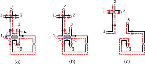
Figure 18. Untying a vertex of degree 6. In part (a) we identify the 6-vertex as untieable. Its key is the cycle $({\overline{3}}\,1\,3)$. To determine the direction of the key (indicated by the dotted line), we start with a leaf (for example, ${\overline{3}}$) and follow the solid line out of it (ignoring the direction of the solid line) which takes us clockwise past the vertex. In part (b) the dotted line indicates how the vertex is to be cut in the untying process. The result of untying is shown in part (c).

An untieable vertex of degree $2m$ can be untied by cutting it into $m$ parts, preserving the solid boundary segments. An example of untying is shown in Fig. 18. The effect of untying on the target permutation is as follows

Lemma 1.

If $\tau$ is the target permutation of an orthogonal diagram, then after untying a vertex with key $\rho$, the target permutation becomes

$$\rho^{-1}\tau\left({\overline{\rho}}\right)^{-1},$$

where ${\overline{\rho}}$ is the reversal of the cycle $\rho$.

Example 11.

In Fig. 18 we have a diagram with the target $(1\,2\,3)({\overline{3}}\,{\overline{2}}\,{\overline{1}})$ and key $({\overline{3}}\,1\,3)$. After untying the target is

$$(1\,{\overline{3}}\,3)(1\,2\,3)({\overline{3}}\,{\overline{2}}\,{\overline{1}})({\overline{3}}\,3\,{\overline{1}})=(1\,2)(3)({\overline{3}})({\overline{2}}\,{\overline{1}}),$$

which can be verified by inspecting the result in Fig. 18(c).

In the unitary case the definition of the untieable vertex and its key is identical to the orthogonal case. However, due to the symmetries of the diagram, the key is composed of labels either all with a bar or all without bar. In the former case we call the vertex $i$-untieable, in the latter $o$-untieable.

Lemma 2.

If $\tau$ is the reduced target permutation of a unitary diagram, then after untying a vertex with key $\rho$, the reduced target permutation becomes

$$\begin{cases}\rho^{-1}\tau,&\mbox{$i$-untying},\\ \tau{\overline{\rho}}^{-1},&\mbox{$o$-untying},\end{cases}$$

where ${\overline{\rho}}$ is the reversal of the cycle $\rho$.

Remark 2.

Lemma 2 is obtained from Lemma 1 by simply erasing all cycles made of symbols with bars. One can go in the other direction as well, reconstructing the cycles with bars using the palindromic symmetry.

The above lemma further explains the notation we used for the untied versions of the principal diagrams in (11).

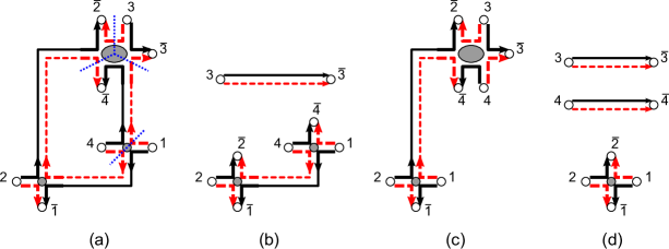
Figure 19. (a) A unitary diagram with two untieable vertices. Untying the 6-vertex leads to (b) while untying the 4-vertex leads to (c). Untying both results in diagram (d).

Example 12.

Consider the diagram in Fig. 19(a). Its reduced target permutation is $(1\,2\,3)(4)$. The vertex of degree 6 is $o$-untieable with the key $({\overline{2}}\,{\overline{4}}\,{\overline{3}})$. After untying, the reduced target of the diagram becomes $(1\,2\,3)(4)(2\,4\,3)=(1\,2\,4)(3)$ as in Fig. 19(b). The vertex of degree 4 is $i$-untieable with the key $(1\,4)$. The reduced target after untying is $(1\,4)(1\,2\,3)(4)=(1\,2\,3\,4)$ depicted in Fig. 19(c). Both can be untied giving $(1\,4)(1\,2\,3)(4)(2\,4\,3)=(1\,2)(3)(4)$ as in in Fig. 19(d).

References

- [1] İ. Adagideli. Ehrenfest-time-dependent suppression of weak localization. Phys. Rev. B, 68:233308, 2003.
- [2] G. Akemann, J. Baik, and P. Di Francesco, editors. The Oxford handbook of random matrix theory. Oxford University Press, Oxford, 2011.
- [3] H. U. Baranger and P. A. Mello. Mesoscopic transport through chaotic cavities: A random S-matrix theory approach. Phys. Rev. Lett., 73:142–145, 1994.
- [4] C. W. J. Beenakker. Random-matrix theory of quantum transport. Rev. Mod. Phys., 69:731–808, 1997.
- [5] C. W. J. Beenakker, J. A. Melsen, and P. W. Brouwer. Giant backscattering peak in angle-resolved Andreev reflection. Phys. Rev. B, 51:13883–13886, 1995.
- [6] G. Berkolaiko, J. M. Harrison, and M. Novaes. Full counting statistics of chaotic cavities from classical action correlations. J. Phys. A, 41:365102, 2008.
- [7] G. Berkolaiko, J. M. Harrison, and M. Novaes. On inequivalent factorizations of a cycle. arXiv:0809.3476, 2008.
- [8] G. Berkolaiko and J. Kuipers. Moments of the Wigner delay times. J. Phys. A, 43:035101, 2010.
- [9] G. Berkolaiko and J. Kuipers. Transport moments beyond the leading order. New J. Phys, 13:063020, 2011.
- [10] G. Berkolaiko and J. Kuipers. Universality in chaotic quantum transport: The concordance between random matrix and semiclassical theories. Phys. Rev. E, 85:045201, 2012.
- [11] G. Berkolaiko and J. Kuipers. Combinatorial theory of the semiclassical evaluation of transport moments I: Equivalence with the random matrix approach. J. Math. Phys., 54:112103, 2013. Preprint, arXiv:1305.4875.
- [12] O. Bernardi. An analogue of the Harer-Zagier formula for unicellular maps on general surfaces. Adv. in Appl. Math., 48:164–180, 2012.
- [13] R. Blümel and U. Smilansky. Classical irregular scattering and its quantum-mechanical implications. Phys. Rev. Lett., 60:477–480, 1988.
- [14] R. Blümel and U. Smilansky. Random-matrix description of chaotic scattering: Semiclassical approach. Phys. Rev. Lett., 64:241–244, 1990.
- [15] P. Braun, S. Heusler, S. Müller, and F. Haake. Semiclassical prediction for shot noise in chaotic cavities. J. Phys. A, 39:L159–L165, 2006.
- [16] P. W. Brouwer and C. W. J. Beenakker. Diagrammatic method of integration over the unitary group, with applications to quantum transport in mesoscopic systems. J. Math. Phys., 37:4904–4934, 1996.
- [17] P. W. Brouwer, K. M. Frahm, and C. W. J. Beenakker. Distribution of the quantum mechanical time-delay matrix for a chaotic cavity. Waves in Random Media, 9:91–104, 1999.
- [18] P. W. Brouwer and S. Rahav. Semiclassical theory of the Ehrenfest time dependence of quantum transport in ballistic quantum dots. Phys. Rev. B, 74:075322, 2006.
- [19] P. W. Brouwer and S. Rahav. Towards a semiclassical justification of the effective random matrix theory for transport through ballistic quantum dots. Phys. Rev. B, 74:085313, 2006.
- [20] M. Büttiker. Four-terminal phase-coherent conductance. Phys. Rev. Lett., 57:1761–1764, 1986.
- [21] G. Chapuy. The structure of unicellular maps, and a connection between maps of positive genus and planar labelled trees. Prob. Theory Related Fields, 147:415–447, 2010.
- [22] G. Chapuy, M. Marcus, and G. Schaeffer. A bijection for rooted maps on orientable surfaces. SIAM J. Discrete Math., 23:1587–1611, 2009.
- [23] T. Engl, J. Kuipers, and K. Richter. Conductance and thermopower of ballistic Andreev cavities. Phys. Rev. B, 83:205414, 2011.
- [24] P. J. Forrester. Quantum conductance problems and the Jacobi ensemble. J. Phys. A, 39:6861–6870, 2006.
- [25] J. Harer and D. Zagier. The Euler characteristic of the moduli space of curves. Invent. Math., 85:457–485, 1986.
- [26] Harish-Chandra. Differential operators on a semisimple Lie algebra. Amer. J. Math., 79:87–120, 1957.
- [27] S. Heusler, S. Müller, P. Braun, and F. Haake. Semiclassical theory of chaotic conductors. Phys. Rev. Lett., 96:066804, 2006.
- [28] C. Itzykson and J. B. Zuber. The planar approximation. II. J. Math. Phys., 21:411–421, 1980.
- [29] D. M. Jackson and T. I. Visentin. An atlas of the smaller maps in orientable and nonorientable surfaces. CRC Press Series on Discrete Mathematics and its Applications. Chapman & Hall/CRC, Boca Raton, FL, 2001.
- [30] Ph. Jacquod and R. S. Whitney. Semiclassical theory of quantum chaotic transport: Phase-space splitting, coherent backscattering and weak localization. Phys. Rev. B, 73:195115, 2006.
- [31] R. A. Jalabert, J.-L. Pichard, and C. W. J. Beenakker. Universal quantum signatures of chaos in ballistic transport. Europhys. Lett., 27:255–258, 1994.
- [32] B. A. Khoruzhenko, D. V. Savin, and H.-J. Sommers. Systematic approach to statistics of conductance and shot-noise in chaotic cavities. Phys. Rev. B, 80:125301, 2009.
- [33] J. Kuipers. Semiclassics for chaotic systems with tunnel barriers. J. Phys. A, 42:425101, 2009.
- [34] J. Kuipers, T. Engl, G. Berkolaiko, C. Petitjean, D. Waltner, and K. Richter. The density of states of chaotic Andreev billiards. Phys. Rev. B, 83:195316, 2011.
- [35] J. Kuipers and K. Richter. Transport moments and Andreev billiards with tunnel barriers. J. Phys. A, 46:055101, 2013.
- [36] J. Kuipers, D. Waltner, C. Petitjean, G. Berkolaiko, and K. Richter. Semiclassical gaps in the density of states of chaotic Andreev billiards. Phys. Rev. Lett., 104:027001, 2010.
- [37] R. Landauer. Spatial variation of currents and fields due to localized scatterers in metallic conduction. IBM J. Res. Dev., 1:223–231, 1957.
- [38] R. Landauer. Spatial variation of currents and fields due to localized scatterers in metallic conduction. IBM J. Res. Dev., 32:306–316, 1988.
- [39] G. Livan and P. Vivo. Moments of Wishart-Laguerre and Jacobi ensembles of random matrices: Application to the quantum transport problem in chaotic cavities. Acta Phys. Pol. B, 42:1081–1104, 2011.
- [40] P. A. Mello. Averages on the unitary group and applications to the problem of disordered conductors. J. Phys. A, 23:4061–4080, 1990.
- [41] J. A. Melsen, P. W. Brouwer, K. M. Frahm, and C. W. J. Beenakker. Induced superconductivity distinguishes chaotic from integrable billiards. Europhys. Lett., 35:7–12, 1996.
- [42] J. A. Melsen, P. W. Brouwer, K. M. Frahm, and C. W. J. Beenakker. Superconductor-proximity effect in chaotic and integrable billiards. Phys. Scr., T69:223–225, 1997.
- [43] F. Mezzadri and N. Simm. Moments of the transmission eigenvalues, proper delay times and random matrix theory I. J. Math. Phys., 52:103511, 2011.
- [44] F. Mezzadri and N. Simm. Moments of the transmission eigenvalues, proper delay times and random matrix theory II. J. Math. Phys., 53:053504, 2012.
- [45] F. Mezzadri and N. Simm. Tau-function theory of quantum chaotic transport with beta=1,2,4. Preprint, arXiv:1206.4584, 2012.
- [46] W. H. Miller. The classical S-matrix in molecular collisions. Adv. Chem. Phys., 30:77–136, 1975.
- [47] S. Müller, S. Heusler, P. Braun, and F. Haake. Semiclassical approach to chaotic quantum transport. New J. Phys., 9:12, 2007.
- [48] S. Müller, S. Heusler, P. Braun, F. Haake, and A. Altland. Semiclassical foundation of universality in quantum chaos. Phys. Rev. Lett., 93:014103, 2004.
- [49] S. Müller, S. Heusler, P. Braun, F. Haake, and A. Altland. Periodic-orbit theory of universality in quantum chaos. Phys. Rev. E, 72:046207, 2005.
- [50] M. Novaes. Statistics of quantum transport in chaotic cavities with broken time-reversal symmetry. Phys. Rev. B, 78:035337, 2008.
- [51] M. Novaes. Semiclassical approach to universality in quantum chaotic transport. EPL, 98:20006, 2012.
- [52] M. Novaes. Combinatorial problems in the semiclassical approach to quantum chaotic transport. J. Phys. A, 46:095101, 2013.
- [53] M. Novaes. A semiclassical matrix model for quantum chaotic transport. J. Phys. A, accepted, 2013.
- [54] V. A. Osipov and E. Kanzieper. Integrable theory of quantum transport in chaotic cavities. Phys. Rev. Lett., 101:176804, 2008.
- [55] V. A. Osipov and E. Kanzieper. Statistics of thermal to shot noise crossover in chaotic cavities. J. Phys. A, 42:475101, 2009.
- [56] C. Petitjean, D. Waltner, J. Kuipers, İ. Adagideli, and K. Richter. Semiclassical approach to the dynamical conductance of a chaotic cavity. Phys. Rev. B, 80:115310, 2009.
- [57] S. Rahav and P. W. Brouwer. Ehrenfest time and the coherent backscattering off ballistic cavities. Phys. Rev. Lett., 96:196804, May 2006.
- [58] K. Richter. Semiclassical theory of mesoscopic quantum systems. Springer, Berlin, 2000.
- [59] K. Richter and M. Sieber. Semiclassical theory of chaotic quantum transport. Phys. Rev. Lett., 89:206801, 2002.
- [60] S. Samuel. integrals, , and the De Wit-’t Hooft anomalies. J. Math. Phys., 21:2695–2703, 1980.
- [61] D. V. Savin and H.-J. Sommers. Shot noise in chaotic cavities with an arbitrary number of open channels. Phys. Rev. B, 73:081307, 2006.
- [62] D. V. Savin, H.-J. Sommers, and W. Wieczorek. Nonlinear statistics of quantum transport in chaotic cavities. Phys. Rev. B, 77:125332, 2008.
- [63] H. Schanz, M. Puhlmann, and T. Geisel. Shot noise in chaotic cavities from action correlations. Phys. Rev. Lett., 91:134101, 2003.
- [64] M. Sieber and K. Richter. Correlations between periodic orbits and their rôle in spectral statistics. Phys. Scr., T90:128–133, 2001.
- [65] H.-J. Sommers, D. V. Savin, and V. V. Sokolov. Distribution of proper delay times in quantum chaotic scattering: A crossover from ideal to weak coupling. Phys. Rev. Lett., 87:094101, 2001.
- [66] W. T. Tutte. Graph theory, volume 21 of Encyclopedia of Mathematics and its Applications. Addison-Wesley, Reading, MA, 1984.
- [67] P. Vivo and E. Vivo. Transmission eigenvalue densities and moments in chaotic cavities from random matrix theory. J. Phys. A, 41:122004, 2008.
- [68] D. Waltner and J. Kuipers. Ehrenfest time dependence of quantum transport corrections and spectral statistics. Phys. Rev. E, 82:066205, 2010.
- [69] D. Waltner, J. Kuipers, Ph. Jacquod, and K. Richter. Conductance fluctuations in chaotic systems with tunnel barriers. Phys. Rev. B, 85:024302, 2012.
- [70] D. Waltner, J. Kuipers, and K. Richter. Ehrenfest-time dependence of counting statistics for chaotic ballistic systems. Phys. Rev. B, 83:195315, 2011.
- [71] D. Weingarten. Asymptotic behavior of group integrals in the limit of infinite rank. J. Math. Phys., 19:999–1001, 1978.
- [72] R. S. Whitney. Suppression of weak localization and enhancement of noise by tunneling in semiclassical chaotic transport. Phys. Rev. B, 75:235404, 2007.
- [73] R. S. Whitney and Ph. Jacquod. Shot noise in semiclassical chaotic cavities. Phys. Rev. Lett., 96:206804, 2006.
- [74] R. S. Whitney and Ph. Jacquod. Controlling the sign of magnetoconductance in Andreev quantum dots. Phys. Rev. Lett., 103:247002, 2009.
- [75] A. Zvonkin. Matrix integrals and map enumeration: an accessible introduction. Math. Comput. Modelling, 26:281–304, 1997.