The Stagger-grid: A grid of 3D stellar atmosphere models

Abstract

Aims. We study the implications of averaging methods with different reference depth scales for 3D hydrodynamical model atmospheres computed with the Stagger-code. The temporally and spatially averaged (hereafter denoted as $\left\langle\mathrm{3D}\right\rangle$) models are explored in the light of local thermodynamic equilibrium (LTE) spectral line formation by comparing spectrum calculations using full 3D atmosphere structures with those from $\left\langle\mathrm{3D}\right\rangle$ averages.

Methods. We explored methods for computing mean $\left\langle\mathrm{3D}\right\rangle$ stratifications from the Stagger-grid time-dependent 3D radiative hydrodynamical atmosphere models by considering four different reference depth scales (geometrical depth, column-mass density, and two optical depth scales). Furthermore, we investigated the influence of alternative averages (logarithmic, enforced hydrostatic equilibrium, flux-weighted temperatures). For the line formation we computed curves of growth for ${Fe\textsc{i}}$ and ${Fe\textsc{ii}}$ lines in LTE .

Results. The resulting $\left\langle\mathrm{3D}\right\rangle$ stratifications for the four reference depth scales can be very different. We typically find that in the upper atmosphere and in the superadiabatic region just below the optical surface, where the temperature and density fluctuations are highest, the differences become considerable and increase for higher $T_{\mathrm{eff}}$, lower $\log g$, and lower $\left[\mathrm{Fe}/\mathrm{H}\right]$. The differential comparison of spectral line formation shows distinctive differences depending on which $\left\langle\mathrm{3D}\right\rangle$ model is applied. The averages over layers of constant column-mass density yield the best mean $\left\langle\mathrm{3D}\right\rangle$ representation of the full 3D models for LTE line formation, while the averages on layers at constant geometrical height are the least appropriate. Unexpectedly, the usually preferred averages over layers of constant optical depth are prone to increasing interference by reversed granulation towards higher effective temperature, in particular at low metallicity.

1 Introduction

Theoretical model atmospheres are needed in order to interpret stellar fluxes and derive individual characteristics of stars, like stellar parameters and chemical abundances. In recent decades, successive improvements of the often used one-dimensional (1D) hydrostatic atmosphere models have confirmed their predictive capabilities (see, e.g., Gustafsson et al. 2008) but also highlighted their limitations. In fact, these 1D models make use of several simplifications in favor of computational ease, the most prominent one being the treatment of convection with the mixing-length theory (MLT, Böhm-Vitense 1958; Henyey et al. 1965). The latter entails several free parameters, in particular the free mixing-length parameter, $\alpha_{\mathrm{MLT}}$, which is a priori unknown, hence normally calibrated for the Sun by observations and assumed constant for all stars. Moreover, the calculation of synthetic spectral absorption lines in 1D requires the additional calibration of micro- and macro-turbulence parameters ($\xi_{\mathrm{turb}}$ and $\chi_{\mathrm{turb}}$, respectively) in order to properly account for the contribution of non-thermal convective and turbulent motions to the broadening of spectral line profiles.

Most of the limitations of 1D modeling of convection can be overcome only by performing time-dependent, three dimensional (3D), radiative-hydrodynamical (RHD) calculations (see Nordlund et al. 2009, and references therein). The goal of 3D simulations is to provide realistic ab initio models where stellar surface convection emerges self-consistently from first principles. Compared to 1D models, such 3D RHD models are able, for the Sun in particular, to predict additional observable features of stars associated with stellar surface velocity fields and temperature and density inhomogeneities, e.g. surface granulation pattern, line asymmetries, and center-to-limb variation (CLV; e.g., such as Asplund et al. 2000b; Pereira et al. 2013). To systematically study such properties of stars with a realistic approach, we computed a large grid of 3D models using the Stagger-code, covering a wide range in stellar parameters ($T_{\mathrm{eff}}$, $\log g$, and $\left[\mathrm{Fe}/\mathrm{H}\right]$) for late-type (spectral type FGK) stars (see Magic et al. 2013, hereafter Paper I).

It is advantageous to reduce the relatively large amount of data from the full 3D atmospheric models to temporally and spatially averaged (hereafter $\left\langle\mathrm{3D}\right\rangle$) representations. However, this reduction comes at the expense of physical self-consistency (see Atroshchenko & Gadun 1994). Nonetheless, in this way one can deal with more manageable atmospheric data structures compared to the otherwise enormous amount of information associated with the full 3D models. These mean $\left\langle\mathrm{3D}\right\rangle$ stratifications are usually compared with classical 1D hydrostatic atmosphere models. Nordlund & Stein (2001) point out that the large-amplitude fluctuations in the superadiabatic region (SAR) leads to deviations from the hydrostatic equilibrium. Furthermore, the 3D data sets incorporate quantities emerging from the hydrodynamics and associated with convection itself, such as, self-consistent velocity fields and turbulent pressure, for which there are no physically consistent counterparts in the case of 1D hydrostatic models.

The definition of the $\left\langle\mathrm{3D}\right\rangle$ stratifications is neither unambiguous nor unique, but depends largely on the choice of reference depth scale. When dealing with the analysis of the atmospheric layers above the optical surface, monochromatic or Rosseland optical depth scales are usually considered the appropriate choice since these are the natural reference depth scales that are used to describe radiative transfer processes in the photosphere. On the other hand, the optical depth loses its usefulness somewhat in the very deep optically thick layers below the optical surface, since here the mean free path of photons becomes very short and the radiative transfer insignificant. Therefore, other reference scales are best suited to describing the main properties of the stellar stratification. Also, the bimodal and highly asymmetric distribution of bulk upflows and of downflows in the convective zone complicates the definition of a meaningful unique average value, particularly near the surface, at the transition between convectively unstable and stable regions.

Uitenbroek & Criscuoli (2011) investigated the application of $\left\langle 3\mathrm{D}\right\rangle$ models to spectral line formation. They computed and compared continuum and atomic line intensities and their respective CLV from $\left\langle 3\mathrm{D}\right\rangle$ and 3D models. They conclude that a mean $\left\langle\mathrm{3D}\right\rangle$ stratification is insufficient to represent the full 3D atmosphere model in the light of spectral analysis. As reasons for the latter they list the non-linearity of the Planck function, formation of molecules, and the asymmetry of convective motions.

The present work constitutes the second paper in the Stagger-grid series. Here, we want to explore the following key question: which averaging method leads to the closest $\left\langle 3\mathrm{D}\right\rangle$ representation of a full 3D data set in the light of spectral line formation calculations? Therefore, we investigate spectral line absorption features by probing the latter with fictitious ${Fe\textsc{i}}$ and ${Fe\textsc{ii}}$ lines with different strengths and excitation potentials for different stellar parameters.

2 Averaging 3D models

The 3D models that form the basis of the present work were computed with the Stagger-code. For a general description of our grid of 3D models, we refer the reader to Paper I. In short, the Stagger-code solves the time-dependent, 3D hydrodynamical equations coupled with realistic non-gray radiative transfer. We utilize an updated version of the realistic state-of-the-art equation of state (EOS) by Mihalas et al. (1988). Continuum and sampled line opacity are taken primarily from the MARCS package (Gustafsson et al. 2008, see also references in Paper I). The radiative transfer is solved for nine angles along long characteristics with a slightly modified version of the Feautrier (1964) method. The opacity-binning method with 12 opacity bins is applied to all Stagger-grid models to reduce the computational burden while still accounting for non-gray radiative transfer under the assumption of local thermodynamic equilibrium (LTE); in particular, the effects of scattering are neglected (see Nordlund 1982; Skartlien 2000; Collet et al. 2011). Our simulations are of the so-called box-in-a-star type, and they cover only a small representative volume of stellar surface that typically includes about ten granules horizontally and spans about 14 pressure scale heights vertically. The numerical resolution of the Cartesian grid is $240^{3}$. It features a non-equidistant vertical axis in order to enhance resolution in the layers with the steepest temperature gradients. The vertical boundaries are open, while the horizontal ones are periodic.

2.1 Computing temporal and horizontal averages

We computed various temporal and horizontal averages for a large number of physical quantities of interest. For the spatial (horizontal) averages, we computed $\left\langle\mathrm{3D}\right\rangle$ stratifications by considering four different reference depth scales and averaging the various physical quantities on layers of constant

• geometrical height, $z$;

• column mass density, $m=\int\rho\,dz$;

• Rosseland optical depth, $\tau_{\mathrm{Ross}}=\int(\rho\kappa_{\mathrm{Ross}})\,dz$;

• optical depth at 500 nm, $\tau_{500}=\int(\rho\kappa_{500})\,dz$,

(hereafter denoted by $\left\langle\mathrm{3D}\right\rangle_{z}$, $\left\langle\mathrm{3D}\right\rangle_{m}$, $\left\langle\mathrm{3D}\right\rangle_{\mathrm{Ross}}$, and $\left\langle\mathrm{3D}\right\rangle_{\mathrm{500}}$, respectively), where $\rho$ is the gas density, and $\kappa_{\mathrm{Ross}}$ and $\kappa_{500}$ are the Rosseland mean opacity and opacity at 500 nm, respectively, both defined as cross-sections per unit mass.

The geometrical averages $\left\langle 3\mathrm{D}\right\rangle_{z}$ are easily taken directly from the output of the Stagger-code, since the numerical mesh of this code is Eulerian in nature. For the three other (Lagrangian-like) averages, the original data sets have to be remapped to their respective new reference depth scale by individually interpolating each column of each 3D simulation snapshot (see 2.3). Furthermore, we also considered four additional averages:

• flux-weighted average temperature, $\langle T^{4}\rangle$;

• average brightness temperature at 500nm, $\langle T_{\mathrm{rad}}\rangle$;

• logarithmic average, $\left\langle\mathrm{3D}\right\rangle_{\log}$; and

• enforced-hydrostatic-equilibrium average, $\left\langle\mathrm{3D}\right\rangle_{\mathrm{HSE}}$.

We determine the flux-weighted temperature stratification $\langle T^{4}\rangle$ by evaluating the spatial averages of $T^{4}$, motivated by the Stefan-Boltzmann law for wavelength-integrated radiative flux. The brightness temperature average $T_{\mathrm{rad}}$ is computed using the expression $B_{500}^{-1}\left(\left\langle B_{500}(T)\right\rangle\right)$, where $B_{500}$ and $B_{500}^{-1}$ denote the Planck function at 500 nm and its inverse, respectively (see also Sect. 3.1). The depth-dependent $\langle T_{\mathrm{rad}}\rangle$ thus needs to be interpreted as the equivalent brightness temperature corresponding to the average black-body emission at 500 nm from each layer. For $\left\langle\mathrm{3D}\right\rangle_{\log}$ we define spatial averages of a given 3D variable $X$ as $\exp\left(\left\langle\log{X}\right\rangle\right)$. Finally, since the $\left\langle\mathrm{3D}\right\rangle$ models do not in general fulfill the hydrostatic equilibrium condition (see App. A.2), for the $\left\langle\mathrm{3D}\right\rangle_{\mathrm{HSE}}$ averages we enforce hydrostatic equilibrium by adjusting the density and adjusting the thermodynamic pressure $p_{\mathrm{th}}$ consistently with the EOS, until hydrostatic equilibrium is attained. We emphasize that the proper enforcement of hydrostatic equilibrium requires that one considers both the thermodynamic $p_{\mathrm{th}}$ and turbulent $p_{\mathrm{turb}}$ contributions to total pressure $p_{\mathrm{tot}}$: the gas pressure in the atmosphere is in fact significantly reduced because of the structural support provided by turbulent pressure. Then, a new geometrical depth $z$ is computed (see Eq. 5).

Classical hydrostatic 1D models of stellar atmospheres are often defined and computed on an optical depth scale, since this allows the numerical resolution to be easily adjusted where it is most needed to achieve the highest accuracy in the solution of the radiative transfer equation in the atmospheric layers, both during the modeling itself and during line-formation calculations. Therefore, especially for radiative transfer-oriented applications, these 1D models can be compared most naturally with averages of corresponding 3D models on constant optical depth, $\left\langle\mathrm{3D}\right\rangle_{\mathrm{Ross}}$ or $\left\langle\mathrm{3D}\right\rangle_{\mathrm{500}}$. In Paper I, in particular, we adopted $\left\langle\mathrm{3D}\right\rangle_{\mathrm{Ross}}$ as our standard averaging choice. One of the main reasons we chose $\left\langle\mathrm{3D}\right\rangle_{\mathrm{Ross}}$ over $\left\langle\mathrm{3D}\right\rangle_{\mathrm{500}}$ is that during the scaling of the simulations and the construction of the initial snapshots, the top physical boundary of essentially all models reached up to $\left\langle\log\tau_{\mathrm{Ross}}\right\rangle_{\mathrm{top}}\approx-6.0$ (see Paper I). In contrast, the vertical extent of the simulations in terms of optical depth at $500$ nm varies depending on stellar parameters ($\log g$ in particular) owing to the concomitant variations in opacity at $500$ nm as a function of temperature and density. Therefore, the $\left\langle\mathrm{3D}\right\rangle_{\mathrm{500}}$ models in general require a careful extrapolation at the top to be extended up to $\log\tau_{500}{\approx}-6.0$ (see Sect. 2.4).

While $\left\langle\mathrm{3D}\right\rangle_{\mathrm{Ross}}$ or $\left\langle\mathrm{3D}\right\rangle_{\mathrm{500}}$ represent natural reference depth scales for the mean photospheric stratification, $\left\langle\mathrm{3D}\right\rangle_{z}$ or $\left\langle\mathrm{3D}\right\rangle_{m}$ is better suited to describing the average physical conditions below the stellar surface; e.g., only the geometrical averages fulfill conservation of momentum and energy (see App. A.2).

In late-type stellar atmospheres, the continuum opacity $\kappa_{\lambda}$ in the optical is dominated by the $\mathrm{H}^{-}$ bound-free absorption that is sensitive to temperature ($\sim T^{10}$). Therefore, even small fluctuations in $T$ will result in large variations in $\kappa_{\lambda}$, which in turn will lead to a high degree of spatial corrugation of layers at constant optical depth (see Stein & Nordlund 1998). Furthermore, owing to such highly non-linear behavior of the $\mathrm{H}^{-}$ opacity, temperature fluctuations around the average will be reduced by interpolation to layers of constant optical depth (see Sect. 4.1).

We note briefly that only the geometrical averages $\left\langle\mathrm{3D}\right\rangle_{z}$, sampled over a sufficient time length, preserve the conservation properties of the hydrodynamical equations, such as hydrostatic equilibrium and conservation of energy. Furthermore, depending on the intended particular application of $\left\langle\mathrm{3D}\right\rangle$ models, it is very important to use these carefully, since the different types of $\left\langle\mathrm{3D}\right\rangle$ models vary significantly among the different averaging methods.

2.2 Basic averaging procedure

We proceeded with the following steps in order to obtain the $\left\langle\mathrm{3D}\right\rangle$ models:

1. Retrieval of 3D variables of interest;

2. Interpolation to new reference depth scale;

3. Computation of horizontal averages and statistics;

4. Extrapolation of horizontal averages, if necessary;

5. Computation of temporal averages.

In case of the geometrical averages $\left\langle\mathrm{3D}\right\rangle_{z}$, steps 2 and 4 are unnecessary and are therefore skipped. Owing to the generally non-linear response of the various physical quantities as a function of basic independent variables and the EOS, the interpolation to a new reference depth scale should be performed after retrieving the variables. In particular, because of these non-linearities, we caution against the derivation of thermodynamic variables via the EOS by utilizing averaged independent variables interpolated to the new reference depth scale, since the spatial averaging will inevitably break the physical self-consistency present in the full original 3D data (see Sect. 2.3 and Appendix A.3).

At the vertical boundaries of our simulation box are so-called ghost zones, each consisting of five layers at the top and bottom. Their sole purpose is to numerically define the boundary conditions at both vertical ends. They do not contain physically meaningful values, so we excluded them before the averaging procedure.

To speed up the calculations without noticeably degrading the statistical properties, when computing the averages we considered only every fourth column of the 3D data cubes in both horizontal directions ($x$ and $y$), which means that the initial $N_{x}N_{y}=240^{2}$ columns are reduced down to $60^{2}$. The vertical extent of the columns is unchanged with $N_{z}=230$ (geometrical) or $101$ (all other reference depth scales). Tests ensured that this horizontal reduction does not influence the horizontal averages owing to the still large sample of vertical columns considered and the multiple snapshots included in the temporal averaging.

For step 3, we used an arithmetic mean to compute the average values of variable $X$ for snapshot $t$ at each horizontal layer $z$:

$$\left\langle X\right\rangle_{z,t}=\frac{1}{N_{x}N_{y}}\sum_{x=1}^{N_{x}}\sum_{y=1}^{N_{y}}X_{xyz,t}$$ (1)

with $N_{x}$ and $N_{y}$ the number of horizontal elements. For exponentially varying variables like density and pressure, we computed also logarithmic averages, i.e., replacing $X_{xyz}$ with $\log X_{xyz}$ in Eq. 1, denoting the models with $\left\langle\mathrm{3D}\right\rangle_{\log}$. In the final step 5, temporal averages are evaluated with

$$\left\langle X\right\rangle_{z}=\frac{1}{N_{t}}\sum_{t=1}^{N_{t}}\left\langle X\right\rangle_{z,t}$$ (2)

with $N_{t}\approx 100-150$ being the total number of snapshots considered for each simulation, which corresponds typically to about two turnover times. In the present work, the combined temporal and spatial averages of variable $X$ are always denoted with $\left\langle X\right\rangle_{\tilde{z}}$, where $\tilde{z}$ is the considered reference depth scale.

Since the 3D structures display a great plethora of details, for each relevant 3D variable we also determine a number of additional statistical properties (standard deviation $\sigma$, root mean square, minimum-maximum range, and histograms of the distribution of values) at each horizontal layer, which are presented and discussed in Sect. 4. As for the spatial averages, the standard deviation and the root mean square are evaluated in step $3$ for each layer $z$ using the same basic expression as in Eq. 1 and, if necessary, doubly extrapolated at the top as in steps 2 and 4 (see Sect. 2.4). Finally, their temporal averages are computed in step 5.

Histograms of the distribution of values we determined separately, and we use temporal averages of the depth-dependent extrema of variable $X$, $\left\langle\min X\right\rangle_{z}$ and $\left\langle\max X\right\rangle_{z}$ to define a depth-dependent range $r_{z}=\left[\left\langle\min X\right\rangle_{z},\left\langle\max X\right\rangle_{z}\right]$ for the histograms. For the 3D variable $X$ at time $t$, we determined a set of 1D histograms, $p_{r,z,t}\left(X\right)$, for each individual layer $z$. The depth-dependent range $r_{z}$ is resolved with $N_{r}=200$ equidistant points; temporal averages $p_{r,z}\left(X\right)$ of the histograms are computed using a subset of $N_{t}=20$ equidistant snapshots (see Sect. 4.3 for details).

Finally, we also computed averages and associated statistical properties separately for up- and downflows, which we differentiate based on the sign of the vertical component of the velocity. Of course, when computing such averages and statistics, one has to account for the correct filling factor in either case, i.e. for the number of elements $N_{x,y}$ belonging to up- or downflows, respectively (Sect. 4.2).

2.3 Interpolation to the new reference depth scale

To interpolate to the new reference depth scale (hereafter denoted as $\tilde{z}$) in step 2, we defined a new equidistant logarithmic reference optical depth scale, $\tilde{z}=\log\tilde{\tau}$, from $-5.0,\dots,+5.0$ in steps of $0.1$ for both optical depth scales $\tau_{\mathrm{Ross}}$ and $\tau_{500}$. In the case of averaging based on the column-mass density scale $m$, we used the column-mass density $\tilde{m}$ normalized to the mean value of $m$ at the optical surface, i.e. $\tilde{z}=\log(\tilde{m})=\log(m/\left\langle m\right\rangle_{\mathrm{surf}})$ for the new reference depth scale, where $\left\langle m\right\rangle_{\mathrm{surf}}$ was determined at $\left\langle\tau_{\mathrm{Ross}}=0\right\rangle$ and considered a fixed range from $-3.0,\dots,+2.0$ in steps of 0.05 for all simulations. All variables, $X$, we remapped column-wise from the original geometrical depth scale to the new reference depth scale, namely $X_{xy}\left(z\right)\rightarrow\tilde{X}_{xy}\left(\tilde{z}\right)$. We use linear interpolation, since quadratic interpolation introduced numerical artifacts in some $\left\langle\mathrm{3D}\right\rangle$ models.

We note that owing to the remapping to a new reference depth scale, points at a constant optical depth or column-mass density will end up probing and spanning a range of geometrical depths, implying that the averages (and statistical properties) with respect to the new reference depth scale will be qualitatively and quantitatively different from plain horizontal averages on constant geometrical depth (see App. A).

2.4 Extrapolation at the top

The vast majority of Stagger-grid models are sufficiently extended vertically, in particular at the top, to embrace the full range of $\log\tilde{\tau}$ with $\left[-5.0,+5.0\right]$. The condition $\left\langle\log\tau_{\mathrm{Ross}}\right\rangle_{\mathrm{top}}\leq-6.0$, is usually fulfilled for all but a few models. More specifically, surfaces of constant optical depth can become quite corrugated at the top for some giant models and fall outside the physical domain of the simulations; that is, one can occasionally have $\log\tau_{\mathrm{Ross}}^{\mathrm{top}}>-5.0$ for a limited number of columns. These particular columns are therefore linearly extrapolated to $\log\tau_{\mathrm{Ross}}=-5.0$ to allow calculating of average quantities in the desired range of optical depths. Exponentially varying values like density, pressure opacities are extrapolated by considering their logarithmic values. The extrapolation is needed only for a few giant models ($\log g\leq 2.5$), and the concerned columns are usually only a small fraction ($\lesssim 0.3\%$). Therefore, we regard these extrapolations as negligible in the case of the optical depth scale $\tau_{\mathrm{Ross}}$.

For the optical depth scale $\tau_{500}$, the situation is slightly different. The mean optical depth at 500 nm at the top $\left\langle\log\tau_{500}\right\rangle_{\mathrm{top}}$ deviates increasingly towards giant models from $\left\langle\log\tau_{\mathrm{Ross}}\right\rangle_{\mathrm{top}}$, so that $\left\langle\log\tau_{500}\right\rangle_{\mathrm{top}}>-5.0$. Therefore, the necessary extrapolation at the top is considerable, in particular for giant models.

We notice that careless column-wise extrapolation at the top can lead to a largely uncertain and erroneous stratification, which would have a negative impact on spectral line formation. For instance, a wrong density stratification at the top can dramatically affect the ionization balance. To limit these extrapolation errors, we first restrict the column-wise extrapolation to the region $\log\tilde{\tau}_{\mathrm{500}}\geq\log\tilde{\tau}_{\mathrm{top}}$ where the value $\log\tilde{\tau}_{\mathrm{top}}>-5.0$ is chosen so that no more than $20\%$ of the columns would require extrapolation up to that level. We then compute the horizontal averages (step 3) and, after that, linearly extrapolate the $\left\langle\mathrm{3D}\right\rangle$ models a second time to the original $\log\tilde{\tau}_{\mathrm{top}}=-5.0$ for each time snapshot. This particular extrapolation procedure produces more plausible stratifications since the horizontal $\left\langle\mathrm{3D}\right\rangle$ averages exhibit a smooth and monotonic behavior with depth at the top compared to individual columns of the 3D data set.

Test calculations of data sets from the solar simulation, which were truncated at the top, revealed the reliability of this double extrapolation approach, since for the temperature stratifications we find the maximum error around $1\,\%$ at the top ($\log\tilde{\tau}_{\mathrm{top}}=-5.0$). Nonetheless, we favor the use of averages on mean Rosseland optical depth, i.e. $\left\langle\mathrm{3D}\right\rangle_{\mathrm{Ross}}$ rather than $\left\langle\mathrm{3D}\right\rangle_{\mathrm{500}}$, since these averages are not plagued by such extrapolation uncertainties. For the extrapolated models on $\tau_{500}$, we kept track of the extent of the applied extrapolation; in fact, only a few models with the lowest gravities ($\log g=1.5/2.0$) exhibit a noteworthy extrapolation ($\log\tilde{\tau}_{\mathrm{top}}\simeq-4.3/4.8$, respectively). The $\left\langle\mathrm{3D}\right\rangle_{\mathrm{500}}$ averages can therefore be reduced to the extrapolation-free regime at the top afterwards.

3 Comparison of the averaging methods

In the following, we systematically compare the different types of averaging procedures explained in Sect. 2 over a broad range of stellar parameters relative to Rosseland optical depth, i.e. $\left\langle\mathrm{3D}\right\rangle_{\tilde{z}}-\left\langle\mathrm{3D}\right\rangle_{\mathrm{Ross}}$. For the sake of clarity, we illustrate the properties of average stratifications only for a representative selection of Stagger-grid models comprising dwarfs and giants ($\log g=4.5$ and $2.0$) at solar and subsolar metallicity ($\left[\mathrm{Fe}/\mathrm{H}\right]=0.0$ and $-3.0$). Besides the most important thermodynamic state variables, temperature and density, we also investigate averages of electron number density, an important quantity for, say, calculations of ionization balance and spectral line formation.

Owing to the lack of a unique common global depth scale that is invariant between different averaging methods, we display their results jointly on the averaged Rosseland optical depth scale, $\left\langle\tau_{\mathrm{Ross}}\right\rangle$, in order to enable a direct comparison.

3.1 Temperature

Figure 1: Relative differences in the temperature (left) and density (right panel) stratification vs. the (averaged) Rosseland optical depth for various stellar parameters. The differences are relative to the Rosseland optical depth, i.e. $\left\langle\mathrm{3D}\right\rangle_{\tilde{z}}-\left\langle\mathrm{3D}\right\rangle_{\mathrm{Ross}}$. Orange/brown dashed lines: averages on layers of constant geometrical height $\left\langle\mathrm{3D}\right\rangle_{z}$; orange/brown dotted lines: averages on layers of constant column mass density $\left\langle\mathrm{3D}\right\rangle_{m}$; orange/brown solid lines: 1D MLT models. Blue solid lines: flux-weighted $T^{4}$-stratifications; blue dashed lines: brightness temperatures $T_{\mathrm{rad}}$ averaged on surfaces of constant Rosseland optical depth (left panel). Green solid lines: logarithmic density averages $\left\langle\mathrm{3D}\right\rangle_{\mathrm{Ross}}^{\mathrm{log}}$; green dashed lines: hydrostatic averages $\left\langle\mathrm{3D}\right\rangle_{\mathrm{Ross}}^{\mathrm{HSE}}$ (right panel). We compare always cooler and hotter effective temperatures, which are distinguished by dark and bright colors respectively. We note that the cool metal-poor dwarfs exhibit very small differences, and are therefore indistinguishable. Note the differences in the $y$-axes.

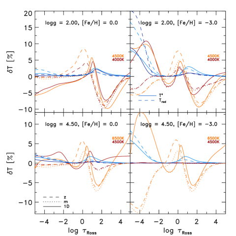
We find that the temperature stratifications of the two optical reference depth scales, $\left\langle\mathrm{3D}\right\rangle_{\mathrm{Ross}}$ and $\left\langle\mathrm{3D}\right\rangle_{\mathrm{500}}$, are similar, therefore we refrain from showing these. Only at the top of the metal-poor stars do the $\left\langle\mathrm{3D}\right\rangle_{\mathrm{500}}$-averages appear cooler ($\sim 5\,\%$, i.e by $\gtrsim 250\,\mathrm{K}$ at $T_{\mathrm{eff}}=6000\,\mathrm{K}$). On the other hand, the geometrical $\left\langle\mathrm{3D}\right\rangle_{z}$ and column mass density $\left\langle\mathrm{3D}\right\rangle_{m}$ averages deviate distinctively from the $\left\langle\mathrm{3D}\right\rangle_{\mathrm{Ross}}$-stratification (see Fig. 1). In the regime $1.0<\log\tau_{\mathrm{Ross}}<3.0$, both $\left\langle\mathrm{3D}\right\rangle_{z}$ and $\left\langle\mathrm{3D}\right\rangle_{m}$ are cooler by $\sim 5-10\,\%$. At the surface ($\tau_{\mathrm{Ross}}=0$), the geometrical averages deviate considerably, while the $\left\langle\mathrm{3D}\right\rangle_{m}$-averages are closer to the optical depth scale (see Fig. 1). In the deeper layers below the superadiabatic regime (SAR), the various averaging methods are practically indistinguishable. In the upper atmosphere the differences are smaller at higher $\left[\mathrm{Fe}/\mathrm{H}\right]$ due to relatively low horizontal contrast, but, these increase significantly for lower metallicity. The averages $\left\langle\mathrm{3D}\right\rangle_{z}$ and $\left\langle\mathrm{3D}\right\rangle_{m}$ are marginally cooler than $\left\langle\mathrm{3D}\right\rangle_{\mathrm{Ross}}$ by $\sim 1-2\,\%$ at solar metallicity. In the metal-poor case $\left[\mathrm{Fe}/\mathrm{H}\right]=-3.0$, the temperature stratifications are distinctively cooler, which will certainly influence the line formation calculations with $\left\langle\mathrm{3D}\right\rangle$ stratifications. Furthermore, the differences increase with higher $T_{\mathrm{eff}}$ and lower $\log g$.

As mentioned earlier, in the atmospheres of late-type stars, minor temperature fluctuations are amplified disproportionally into large variations in the line and continuum opacity $\kappa_{\lambda}$ owing to the strong $T$-sensitivity of the $\mathrm{H}^{-}$-opacity ($\kappa_{\lambda}{\propto}T^{10}$, see Stein & Nordlund 1998). Therefore, surfaces of constant optical depth appear strongly corrugated in terms of the range of geometrical heights that they span. The transformation to layers of constant optical depth will naturally even out these corrugated surfaces and, at the same time, smooth the temperature fluctuations, since the latter are the source of the former (see App. A.1). Therefore, these are noticeably smaller on layers of constant optical depth compared to layers of constant geometrical depth, which is portrayed in the temperature contrast and histogram (see also Figs. 3 and 6). The SAR exhibits large-amplitude fluctuations as a result of the release of thermal and ionization energy at the photospheric transition, which are the reason for the observed enhanced differences between the averaging methods (see Sect. 4.1).

Steffen & Holweger (2002) found a beneficial mean $\left\langle T\right\rangle$-representation for the Sun in the flux-weighted temperature averages, $T^{4}$, taken on constant Rosseland optical depth from their 2D simulations. The idea behind this approach is that the $T^{4}$-averages render radiation-oriented $T$-stratifications, therefore resulting in 1D line profiles that are closer to the multidimensional ones (see also Steffen et al. 1995). To allow for a similar comparison for our models, we computed such average $T^{4}$-stratifications. In Fig. 1, the $T_{\mathrm{Ross}}^{4}$-stratifications generally appear hotter at the top and in the SAR compared to the simple $T$-stratification. Averages taken at the fourth power will weight higher values more, which leads to hotter average temperatures. This could lead to pronounced differences for molecular lines that form high up in the atmosphere. At solar metallicity, the $T^{4}$-stratifications at the top are fairly similar to the plain $T$-averages ($\sim 1-2\,\%$) in agreement with the findings of Steffen & Holweger (2002). This is different at lower metallicity ($\left[\mathrm{Fe}/\mathrm{H}\right]=-3.0$), namely the $T^{4}$-averages are clearly higher by $\sim 5-10\,\%$. At higher $T_{\mathrm{eff}}$ and lower $\log g$, the temperature differences are greater, in particular for the metal-poor giants, owing to the enhanced temperature fluctuations (see Sect. 4.1).

Under the assumption of local thermodynamic equilibrium (LTE) and neglecting the effects of scattering, the source function is given by the Planck function, $S_{\lambda}=B_{\lambda}\left(T\right)$. Within this approximation, we can thus consider the brightness temperature average $T_{\mathrm{rad}}$ defined earlier in Sect. 2.1 as a good representation of the mean temperature stratification from the point of view of the radiative emission properties: brighter parts in each depth layer are given more weight with this averaging method. The differences between the average $T_{\mathrm{rad}}$ at $500\,\mathrm{nm}$ and average $T$-stratifications are displayed in Fig. 1. Their variations with stellar parameters are very similar to those of $T^{4}$-averages, however, slightly more pronounced, in particular the metal-poor giants exhibit hotter stratifications by up to $\sim 20\,\%$ at the top.

3.2 Density

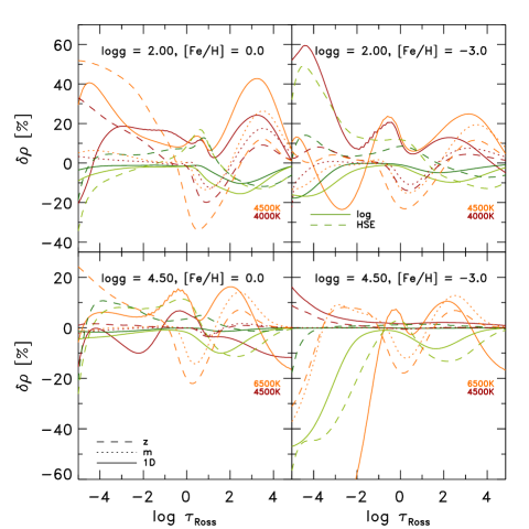
In Fig. 1, we also illustrate the results of averaging in the case of the density stratifications. In the deeper interior, the different $\left\langle\mathrm{3D}\right\rangle$ models converge toward the same density stratification. In the SAR, below the optical surface at $\log\tau_{\mathrm{Ross}}\gtrsim 0.0$, the geometrical averages $\left\langle\mathrm{3D}\right\rangle_{z}$ are smaller than the $\left\langle\mathrm{3D}\right\rangle_{\mathrm{Ross}}$ averages by up to $\sim 30\,\%$, while at the top these are much denser by up to $\sim 40\,\%$. The differences increase towards higher $T_{\mathrm{eff}}$ and lower $\log g$. We find a different behavior in the metal-poor dwarfs, which turn lower towards the top after the initial increase ($\sim 10\,\%$). The density stratifications averaged on column mass density $\left\langle\mathrm{3D}\right\rangle_{m}$ are larger in the SAR and in the upper layers closer to $\left\langle\mathrm{3D}\right\rangle_{\mathrm{Ross}}$. However, we find that at lower metallicity $\left\langle\rho\right\rangle_{m}$ they are smaller by up to $\sim 30\,\%$. We note that thermal pressure qualitatively shows the same characteristics as the density.

The shape of the density distribution is symmetric and narrow on layers of constant column mass density, thanks to the exponential stratification of the atmosphere and to the additional damping of density fluctuations on the column mass scale (see Fig. 6). As a result, the $\left\langle\mathrm{3D}\right\rangle_{m}$ averages feature the narrowest contrast and density ranges, which, on the contrary, are usually greatest for geometrical averages $\left\langle\mathrm{3D}\right\rangle_{z}$; for the $\left\langle\mathrm{3D}\right\rangle_{\mathrm{Ross}}$ averages, these are noticeably reduced due to the mapping onto the optical reference depth scale (Fig. 3). Overall, the density fluctuations at the top of the $\left\langle\mathrm{3D}\right\rangle_{\mathrm{Ross}}$ stratifications are similarly as small as those by $\left\langle\mathrm{3D}\right\rangle_{m}$ and $\sim 20\,\%$; however, for metal-poor dwarfs they reach up to $\sim 80\,\%$ (see Fig. 3). As shown in Sect. 4.3, we find that the corrugation of the layers of constant optical depth in the upper part of 3D model stellar atmospheres at lower metallicity increases considerably towards higher $T_{\mathrm{eff}}$ because of an enhanced $T$-contrast by the so-called reversed granulation (see Rutten et al. 2004). This in turn broadens the density distribution during the remapping to the optical depth scale, shifting the mean density value and leading to the observed deviations between $\left\langle\rho\right\rangle_{\mathrm{Ross}}$ and $\left\langle\rho\right\rangle_{m}$ at lower metallicity (see App. A.1), which will affect the $\left\langle\mathrm{3D}\right\rangle$ line formation calculations.

The highly stratified structure of stellar atmospheres features an exponential decrease with height. Linear density averages will therefore tend to give more weight to higher density values, leading to a systematic overestimation of the mean densities. For this reason we consider the logarithmic averages $\left\langle\rho\right\rangle_{\mathrm{log}}$, which we compare to the linear ones in Fig. 1. As expected, we find the logarithmic $\rho$-averages are smaller than the linear ones, with the difference between the two increasing with higher $T_{\mathrm{eff}}$ and lower $\log g$ by up to $\sim 30\,\%$. The mean densities in the upper layers are lower by $\sim 10\,\%$ and $\sim 40\,\%$ at solar and low metallicity, respectively. For quantities that vary more moderately (e.g., temperature) the differences between logarithmic and linear averaging are rather small.

The transformation to constant optical depth and the subsequent averaging will change the physical self-consistency as shown in App. A.2. To rectify this, we followed the recommendation of Uitenbroek & Criscuoli (2011) and also computed $\rho$-stratifications, which are enforced to be in hydrostatic equilibrium, $\left\langle\rho\right\rangle_{\mathrm{HSE}}$ (Fig. 1). These deviate significantly from the plain $\left\langle\rho\right\rangle$-stratifications, in particular at the top. Incidentally, we note however that their dynamic nature and the effects of convective flows and turbulent pressure mean that the 3D models themselves are not strictly speaking in hydrostatic equilibrium at any one time.

In Fig. 1 (both panels), we also compare the 1D MLT models with the $\left\langle\mathrm{3D}\right\rangle_{\mathrm{Ross}}$ stratifications. The 1D models in general show qualitatively similar behavior as the geometrical averages. The metal-poor 1D models are distinctively hotter, since these enforce radiative equilibrium in the upper layers.

3.3 Electron number density

Figure 2: Root mean square (rms) of the vertical velocity $v_{z,\mathrm{rms}}$ (left) and mean electron number density $n_{\mathrm{el}}$ vs. optical depth (right panel). Dashed lines: $\left\langle\mathrm{3D}\right\rangle_{z}$ averages; dotted lines: $\left\langle\mathrm{3D}\right\rangle_{m}$; solid lines: $\left\langle\mathrm{3D}\right\rangle_{\mathrm{Ross}}$.

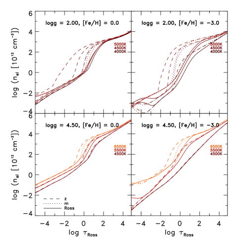
We find large differences among the various averages of the electron number density, $n_{\mathrm{el}}$, which we show in Fig. 2 (right panel). In the SAR the geometrical averages $\left\langle n_{\mathrm{el}}\right\rangle_{z}$ are distinctively larger than the averages on surfaces of constant Rosseland optical depth $\left\langle n_{\mathrm{el}}\right\rangle_{\mathrm{Ross}}$, while the column mass density averages $\left\langle n_{\mathrm{el}}\right\rangle_{m}$ are found in between the two. The deviations increase for higher $T_{\mathrm{eff}}$ and lower $\log g$ considerably, while at lower $T_{\mathrm{eff}}$ the differences are significantly smaller. We show in App. A.1 that the interpolation to a new reference depth scale changes the statistical properties by redistributing properties from different heights, so the resulting mean horizontal average will look different depending on the reference depth scale. This effect seems to be most pronounced in the case of electron density.

To determine the ionization fraction in spectral line calculations, the electron number density is either already provided by the model atmosphere or looked up from an EOS using the independent thermodynamic variables (typically $(T,p)$ or $(T,\rho)$). The latter has to be done carefully in the case of the $\left\langle\mathrm{3D}\right\rangle$ models, since, besides potential differences in the EOS compared to the one used for calculating the model atmosphere, electron densities derived from the EOS based on averaged independent variables, $n_{\mathrm{el}}^{\mathrm{EOS}}=n_{\mathrm{el}}\left(\left\langle T\right\rangle,\left\langle p\right\rangle\right)$, can deviate significantly from the more physically consistent averaged $\left\langle n_{\mathrm{el}}\right\rangle$ (see App. A.3).

3.4 Vertical velocity

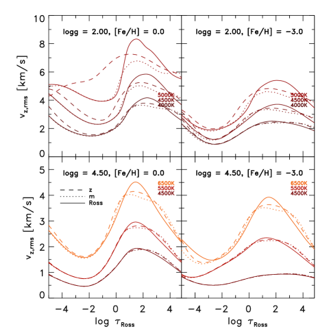
It is worthwhile to compare how the vertical velocity, $v_{z,\mathrm{rms}}$, changes with the respective averaging methods. For comparison, we show in Fig. 2 (left panel) the rms of the vertical velocity. In the upper layers, we find the $v_{z,\mathrm{rms}}$ on geometrical averages to be higher compared to other averages, while it is lower in the deeper layers. On optical depth the peak in $v_{z,\mathrm{rms}}$ below the surface is somewhat symmetric and slightly higher, while for averages on geometrical height and column mass density their peaks are flatter and more skewed towards higher layers, and the peak location is realized in slightly upper layers. For lower $T_{\mathrm{eff}}$ and higher $\log g$, the differences diminish more and more, so that for the coolest models, the difference are small. The differences in the velocity arise as well due to the redistribution of velocity during the mapping to the new reference depth scale (see App. A.1).

4 Statistical properties

To explore the origins of the differences among the various average $\left\langle\mathrm{3D}\right\rangle$ structures and the resulting ramifications for line formation calculations, we discuss here the statistical properties of the temperature, density, and velocity stratifications. Since the statistical properties of $\left\langle\mathrm{3D}\right\rangle_{\mathrm{500}}$ and $\left\langle\mathrm{3D}\right\rangle_{\mathrm{Ross}}$ are fairly similar, we focus only on the latter.

4.1 Contrast

Figure 3: Temperature (top) and density (bottom) contrasts vs. averaged Rosseland optical depth. Dashed lines: $\left\langle\mathrm{3D}\right\rangle_{z}$ averages; dotted lines: $\left\langle\mathrm{3D}\right\rangle_{m}$; solid lines: $\left\langle\mathrm{3D}\right\rangle_{\mathrm{Ross}}$.

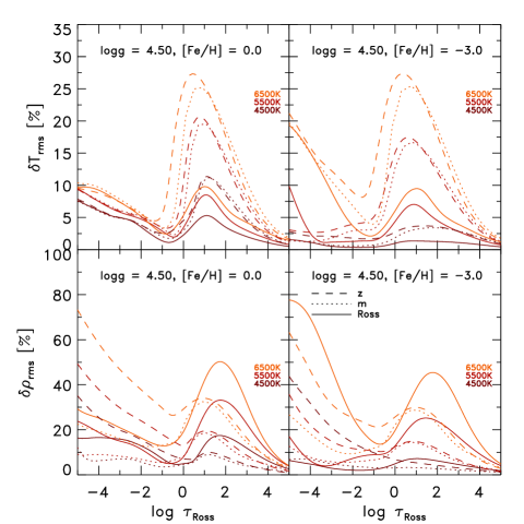
The 3D RHD models usually exhibit a broad range of values at a given height thanks to the fluctuations arising from the convective motions. The amplitude of these fluctuations can be quantified using the root-mean-square of the relative deviation from the mean,

$$\delta X_{\mathrm{rms}}=\sqrt{\Sigma_{i=1}^{N}\left(X_{i}-\bar{X}\right)^{2}/\left(N\bar{X}^{2}\right)},$$ (3)

which we refer to as the contrast ($\bar{X}$ is the mean value of $X$). It is equal to the normalized standard deviation; i.e., $\delta X_{\mathrm{rms}}=\sigma_{X}/\bar{X}$.

The translation to another reference depth scale changes the statistical properties as variables are remapped, which in turn is reflected in changes in contrast. Among the various averaging methods, geometric averages $\left\langle\mathrm{3D}\right\rangle_{z}$ typically feature the highest contrast. We also find that the level of fluctuations generally increases with increasing $T_{\mathrm{eff}}$ and decreasing $\log g$. The highest contrast typically prevails in simulations with the highest $T_{\mathrm{eff}}$ and located in the vicinity of the maximum superadiabatic gradient, $\@vec{\nabla}_{\mathrm{sad}}^{\mathrm{peak}}$, and maximum rms-velocity, $v_{z,\mathrm{rms}}^{\mathrm{peak}}$. These arise from the photospheric transition from convective to radiative energy transport, and the resulting overturning of the entropy-depleted plasma. At the top of the convection zone, the fluctuations reach a minimum, and they decrease towards the bottom of the model atmosphere.

In top and bottom panels of Fig. 3, we show the temperature and density contrasts, $\delta T_{\mathrm{rms}}$ and $\delta\rho_{\mathrm{rms}}$, respectively. In the case of the optical depth $\left\langle\mathrm{3D}\right\rangle_{\mathrm{Ross}}$, the temperature contrast is significantly reduced compared to the other reference depth scales ($\delta T_{\mathrm{rms}}^{\mathrm{peak}}$ reduced by a factor of $\sim 3$), while the density contrast is slightly enhanced ($\delta\rho_{\mathrm{rms}}^{\mathrm{peak}}\sim 20-60\,\%$ compared to $10-50\,\%$). For averages on column mass density $\left\langle\mathrm{3D}\right\rangle_{m}$, $\delta\rho_{\mathrm{rms}}$ is lower, in particular in the upper layers, and $\delta T_{\mathrm{rms}}$ is slightly smaller compared to the $\left\langle\mathrm{3D}\right\rangle_{z}$ case. Fluctuations of variables that correlate with the new reference depth scale will be reduced during the transformation. As the translation to layers of constant optical depth partly evens out the corrugated $\tau$-isosurface, fluctuations of the opacity $\kappa_{\lambda}$ will be reduced, since the dominant $\mathrm{H}^{-}$opacity is very sensitive to temperature. Therefore, the temperature fluctuations are also smoothed out. Layers of constant column mass density will similarly suppress density variations (see App. A.1). At the top, $\delta\rho_{\mathrm{rms}}$ is almost similar between $\left\langle\mathrm{3D}\right\rangle_{m}$ and $\left\langle\mathrm{3D}\right\rangle_{\mathrm{Ross}}$ in the case of the solar metallicity $(\delta\rho_{\mathrm{rms}}^{\mathrm{top}}\sim 40\,\%$); however, at lower metallicity, $\left[\mathrm{Fe}/\mathrm{H}\right]=-3.0$, we find considerable disparity with $\delta\rho_{\mathrm{rms}}^{\mathrm{top}}\sim 80\,\%$.

The thermal stratification in the upper atmosphere is determined by adiabatic cooling thanks to mechanical expansion and radiative heating because of spectral line re-absorption (Asplund et al. 1999; Collet et al. 2007). In metal-poor stars, radiative reheating in upper layers is significantly reduced owing to the weakness of spectral line features, while the mechanical expansion cooling term is virtually unaffected. The reversed granulation takes place at increasingly lower geometrical height with higher $T_{\mathrm{eff}}$ and lower $\log g$, causing the distribution of the thermodynamic variables to become increasingly broader and more skewed (see Sect. 4.3). This is the reason for the enhancement in $\delta T_{\mathrm{rms}}$ and $\delta\rho_{\mathrm{rms}}$ towards the top boundary in metal-poor simulations in Fig. 3. Replicating the results of full 3D line formation calculations in low-metallicity stars with $\left\langle\mathrm{3D}\right\rangle$ models is therefore challenging, since the averages have to correctly account for such temperature and density fluctuations. Interestingly, the temperature contrast saturates at $6500\,\mathrm{K}$, similar to the saturation of the intensity contrast shown in our previous work (see Fig. 10 in Paper I).

The strength of spectral lines is sensitive to temperature, and the remapping to constant optical depth decreases $\delta T_{\mathrm{rms}}$, making $\left\langle T\right\rangle$ closer to $\left\langle T\right\rangle_{\mathrm{rad}}$. However, the transformation to layers of constant optical depth exhibits the side effect of redistributing the other variables, too, in particular the gas density; $\delta\rho_{\mathrm{rms}}$ is thus much higher than averages on column mass density, due to the additional influence of opacity on the depth scale (see Sect. 2.1). This in turn will likely affect the line formation calculations with the different $\left\langle\mathrm{3D}\right\rangle$ models.

The strong contrast in the upper part of the convection zone ($\log\tau_{\mathrm{Ross}}\geq 0$) is induced by the large amplitude fluctuations owing to the radiative energy losses at the photosphere and the asymmetry of the up- and downflows, which we discuss further in Sect. 4.2. An interesting aspect is that the contrast in thermodynamic variables is very similar to the rms of the vertical velocity (Fig. 2), which is indicative of the correlation between the mass flux and the fluctuations in the thermodynamic variables. Namely, vertical velocity is generated by density contrast $\delta\rho$ via to the buoyancy force, $f_{B}=-g\delta\rho$, which results from an imbalance of pressure and gravity terms in the hydrodynamical equation for conservation of momentum (see Paper I) in the highly stratified atmosphere. Lighter fluid elements ($\delta\rho<0$) experience positive buoyancy and thus upward acceleration, while denser elements ($\delta\rho>0$) experience negative buoyancy and are pulled downward. Buoyancy forces will vanish eventually, when the density of the up- or downflowing element levels with the surrounding gas.

The entropy contrast $\delta s_{\mathrm{rms}}$ (not shown here), qualitatively depicts a very similar dependence on stellar parameter and reference depth scale as $\delta T_{\mathrm{rms}}$. Both are very similar in optical depth, while for the averages $\left\langle\mathrm{3D}\right\rangle_{z}$ and $\left\langle\mathrm{3D}\right\rangle_{m}$ the overall amplitude is a factor $\sim 2$ smaller. In Paper I, we showed that the convective energy flux depends on the entropy jump, density, and vertical velocity. Interestingly, here we also find additional scaling relations concerning the peak contrast in entropy, $\delta s_{\mathrm{rms}}^{\mathrm{peak}}$, and density, $\delta\rho_{\mathrm{rms}}^{\mathrm{peak}}$, with the vertical peak velocity $v_{z,\mathrm{rms}}^{\mathrm{peak}}$. This can be interpreted as convective driving, where the radiative losses generate large fluctuations in the entropy, temperature, and density.

For the different averaging methods, the variations in the minimum-maximum range for the temperature and density are qualitatively very similar to the contrast (even though with larger amplitudes $\sim 5-8$), therefore, we refrain from discussing these explicitly.

4.2 Upflows and downflows

Figure 4: Similar as Fig. 3 but showing the relative difference between averages in up and downflows, $\delta T_{\mathrm{up,dn}}$ and $\delta\rho_{\mathrm{up,dn}}$.

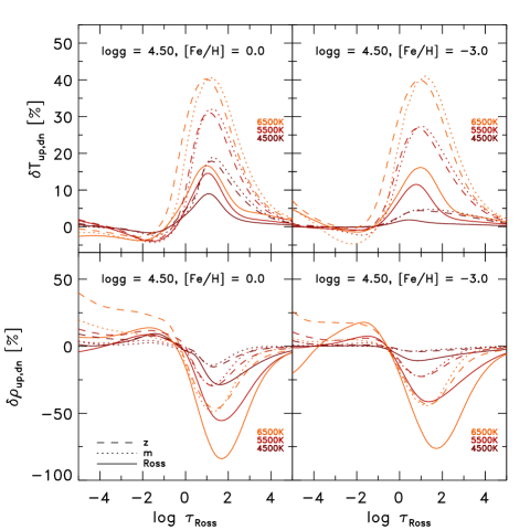
The properties of the convective motions in stellar atmospheres are highly asymmetric in up- and downflows. The upflows overshoot into the photosphere leading to non-thermal Doppler shifts imprinted on spectral line features. We first compute the mean values of various variables separately for up- and downflows based on the sign of the velocity at a given height. We then determine the relative difference between up- and downflows with $\delta X_{\mathrm{up,dn}}=(X_{\mathrm{up}}-X_{\mathrm{dn}})/\bar{X}$ (Fig. 4). As expected, the buoyant upflows are hotter and lighter compared to the subsiding downflows. Furthermore, the asymmetries are especially pronounced in the convection zone below the optical surface. Above the photosphere, the convective motions decay quickly, and the asymmetries in $\delta T_{\mathrm{up,dn}}$ and $\delta\rho_{\mathrm{up,dn}}$ are distinctively smaller. The remaining asymmetries at the top stem from reverse granulation.

The convective flows in granules, slow and almost laminar, radiate away their energy and overturn into the intergranular lanes characterized by cool, dense, narrow turbulent downdrafts. The subsequent large-amplitude fluctuations in the thermodynamical properties are caused by the turbulent mixing of the downflows with the upflows, typically located in the intergranular lane below the optical surface in the SAR. These regions are arranged in tubelike structures around the granules, and can be identified with their excessive vorticity. It is remarkable that, across all stellar parameters, the filling factor of the up- and downflow in the convection zone remains almost constant, with $f_{\mathrm{up}}\sim 2/3$ and $f_{\mathrm{dn}}\sim 1/3$, respectively (see Paper I).

The variable $\delta T_{\mathrm{up,dn}}$ is reduced, and $\delta\rho_{\mathrm{up,dn}}$ is enhanced on the optical reference depth scale $\left\langle\mathrm{3D}\right\rangle_{\mathrm{Ross}}$ compared to the other averages. The column mass density shows a smaller asymmetry in density. This behavior, similar to what we discussed earlier for the temperature and density contrasts, is not entirely surprising, since the fluctuations are caused by the presence of the up- and downflows (see also A.1).

4.3 Histograms

Figure 5: Histogram of the temperature (top) and density (bottom) vs. optical depth for the TO simulation ($T_{\mathrm{eff}}=6500\,\mathrm{K}/\log g=4.0$) with solar and sub-solar metallicity ($\left[\mathrm{Fe}/\mathrm{H}\right]=-3.0$). Additionally, the histogram of a single layer ($\log\tau_{\mathrm{Ross}}=-4.0$) is indicated for the whole layer (black) and separated in up- and downflows (blue and red, respectively). Dashed lines: $\left\langle\mathrm{3D}\right\rangle_{z}$ averages; dotted lines: $\left\langle\mathrm{3D}\right\rangle_{m}$; solid lines: $\left\langle\mathrm{3D}\right\rangle_{\mathrm{Ross}}$; blue solid lines: 1D MLT models.

Figure 6: Histograms of the temperature (left) and density (right panel) distributions taken at $\left\langle\log\tau_{\mathrm{Ross}}\right\rangle=-4.0$. We show the histograms averaged on constant geometrical height (top), column mass density (middle), and Rosseland optical depth (bottom). The surface gravity of displayed models is $\log g=4.5$ and the metallicity is solar (dashed lines) and subsolar with $\left[\mathrm{Fe}/\mathrm{H}\right]=-3.0$ (solid lines). The mean values are indicated by filled and open circles for $\left[\mathrm{Fe}/\mathrm{H}\right]=-3.0$ and 0.0, respectively).

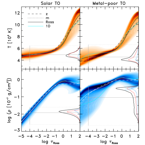
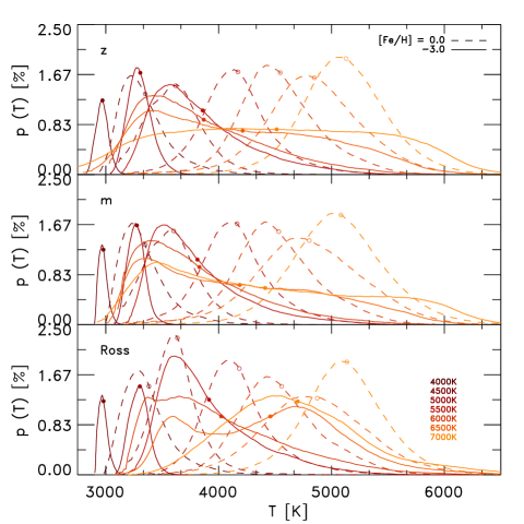
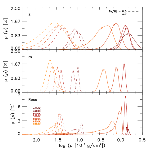
In Fig. 5, we illustrate temporally averaged histograms of the temperature, $p\left(T\right)$, and density distributions, $p\left(\rho\right)$ for the TO simulation with two different $\left[\mathrm{Fe}/\mathrm{H}\right]$ evaluated on layers of constant Rosseland optical depth, in order to illustrate the differences in the statistical properties. The histogram of the metal-poor case differs substantially in upper layers from the solar one. Furthermore, in Fig. 6, we show $p\left(T\right)$ and $p\left(\rho\right)$ in the upper layers ($\left\langle\log\tau_{\mathrm{Ross}}\right\rangle=-4.0$) for dwarf models with different $T_{\mathrm{eff}}$ and $\left[\mathrm{Fe}/\mathrm{H}\right]$. In both cases we compare the distributions on constant geometrical height $z$, constant column mass density $m$ and constant Rosseland optical depth $\tau_{\mathrm{Ross}}$.

At solar metallicity (Fig. 6), the temperature distributions are very narrow and symmetric. With increasing $T_{\mathrm{eff}}$, the average $T$ is as expected higher and the width of the distribution broadens slightly. The mean values are very similar between the different $\left\langle\mathrm{3D}\right\rangle$ methods and in principle indistinguishable, which also agrees with Fig. 1. Furthermore, the mean values are located very close to the mode.

At $\left[\mathrm{Fe}/\mathrm{H}\right]=-3.0$, the temperature distributions change considerably. While at cooler $T_{\mathrm{eff}}$ the shape is vey narrow and symmetric, for $T_{\mathrm{eff}}\geq 5500\,\mathrm{K}$ we find a distinct broadening of the $T$-distribution on geometrical reference depth scale $\left\langle\mathrm{3D}\right\rangle_{z}$, which is given by a long tail at high $T$ and a decreasing peak at lower $T$ (see Figs. 5 and 6). In the column mass density averages $\left\langle\mathrm{3D}\right\rangle_{m}$ the temperature peak is slightly more pronounced at higher $T_{\mathrm{eff}}$, while the high-$T$ tail is slightly reduced. The situation is pretty different for the averages on Rosseland optical depth $\left\langle\mathrm{3D}\right\rangle_{\mathrm{Ross}}$, where we find that the temperature peak drops faster towards higher $T_{\mathrm{eff}}$, and at $7000\,\mathrm{K}$ the $T$-distribution shows an almost unimodal distribution. The mean values disagree at higher $T_{\mathrm{eff}}$ between the different reference depth scales.

The density distributions behave differently depending on the reference depth scale. On $\left\langle\mathrm{3D}\right\rangle_{z}$ the histograms are in general slightly skewed with a fat tail towards lower $\rho$ for all metallicities (Figs. 5 and 6). The density distributions for the averages on column mass density are very symmetric and narrow for both solar and low metallicities. At solar metallicity, the density histograms on constant optical depth are narrower and higher than the geometrical analogs, but skewed in contrast to $\left\langle\mathrm{3D}\right\rangle_{m}$. In the metal-poor case, $\left\langle p\left(\rho\right)\right\rangle_{\mathrm{Ross}}$ becomes very narrow and symmetric at lower $T_{\mathrm{eff}}$, but towards higher $T_{\mathrm{eff}}$ we find the $\rho$-distribution to also be broader. The mean density stratification varies considerably among the different averaging methods.

As mentioned above, adiabatic cooling due to mechanical expansion and radiative reheating are competing with each other in the upper photosphere and contribute to the phenomenon of reversed granulation. At lower metallicity, the reversed granulation is enhanced, so that the optical depth is increasingly strongly corrugated towards higher $T_{\mathrm{eff}}$, which in turn will amplify the differences in statistical properties during the translation to the optical depth scale from the geometrical depth scale. This leads to the systematical broadening in the statistical distribution that we encounter at lower metallicity.

5 Spectral line formation: $\left\langle\mathrm{3D}\right\rangle$ and $3\mathrm{D}$ LTE calculations

Figure 7: Overview of the $\left\langle\mathrm{3D}\right\rangle-3\mathrm{D}$ line formation differences given in abundances displacement $\Delta\log\varepsilon$ vs. equivalent width $W_{\lambda}$ for the ${Fe\textsc{i}}$ and ${Fe\textsc{ii}}$ fictitious spectral lines with the excitation potentials $\chi_{\mathrm{exc}}=1.0$ and $4.0\,\mathrm{eV}$ including the Sun, TO, RG and dwarf simulation (from top to bottom). The averages on layers of constant geometric height $\left\langle\mathrm{3D}\right\rangle_{z}$ (black dashed), constant column mass density $\left\langle\mathrm{3D}\right\rangle_{m}$ (black dotted), constant Rosseland optical depth $\left\langle\mathrm{3D}\right\rangle_{\mathrm{Ross}}$ (black solid) and at 500 nm $\left\langle\mathrm{3D}\right\rangle_{\mathrm{500}}$ (orange dashed triple-dotted lines) are indicated. Furthermore, we show 1D models (red solid), $T_{\mathrm{rad}}^{\mathrm{Ross}}$-averages (blue dashed) and $\left\langle\mathrm{3D}\right\rangle_{\mathrm{Ross}}^{\mathrm{HSE}}$ (green dashed lines). The microturbulence of $\xi_{\mathrm{turb}}=1.0\,\mathrm{km}/\mathrm{s}$ has been used throughout. Notice the different ordinates.

Figure 8: Similar to Fig. 7 but showing overview of the abundance corrections for metal-poor models, with larger ranges for the $y$-scales.

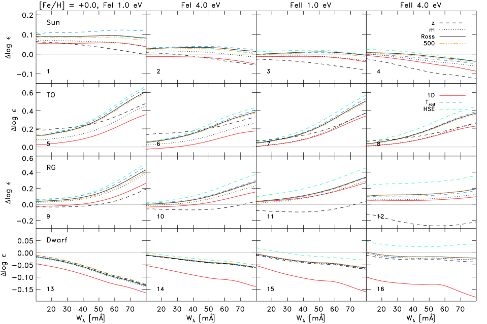
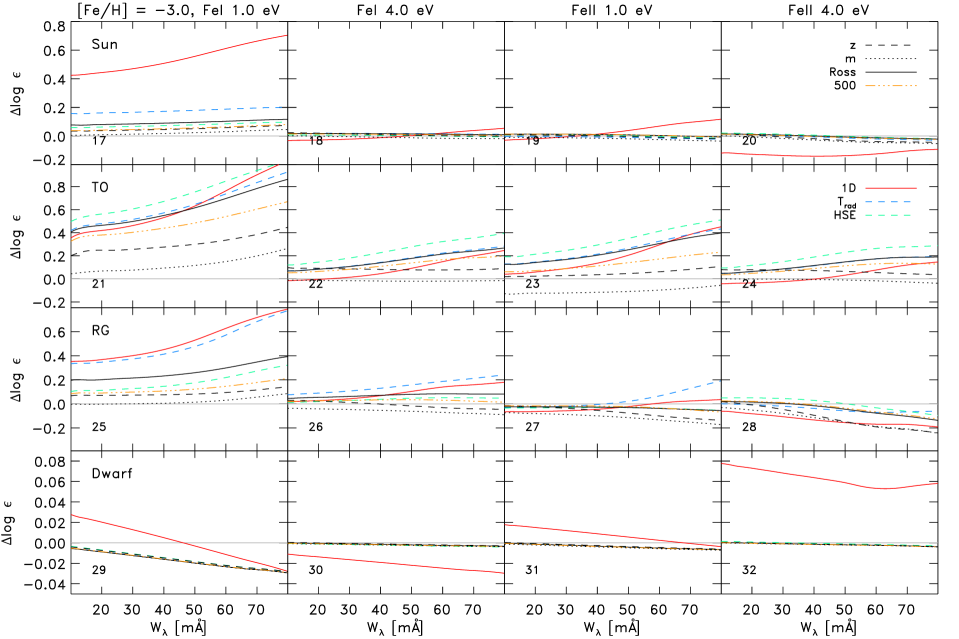
To explore the differences between the line formation based on $\left\langle\mathrm{3D}\right\rangle$ and full 3D models, we have chosen a set of representative models consisting of a main-sequence (MS) star ($T_{\mathrm{eff}}/\log g=5777$ K/$4.44$), a turn-off (TO) star ($6500$/$4.0$), a red-giant (RG) star ($4500$/$2.0$), and a dwarf ($4500/5.0$). For all these models, we considered metal-poor analogs with $\left[\mathrm{Fe}/\mathrm{H}\right]=-3.0$ besides the solar metallicity.

5.1 3D line formation calculations

We used the 3D radiative transfer code Scate (Hayek et al. 2011) to calculate full 3D synthetic spectral line disk-center intensity and flux profiles with 3D Stagger model atmospheres. Scate assumes local thermodynamic equilibrium (LTE). Furthermore, in the present work, we also neglected the effects of scattering; i.e. we approximated the source function with the Planck function, $S_{\lambda}=B_{\lambda}$. We caution that LTE is in general a poor approximation, especially for ${Fe\textsc{i}}$ spectral line formation calculations at low $\left[\mathrm{Fe}/\mathrm{H}\right]$ (e.g. Bergemann et al. 2012), which should be kept in mind for analyzing the LTE-based abundance corrections presented here. For the sake of consistency, we used the same EOS (Mihalas et al. 1988) and continuum opacity data (from the MARCS package; see Gustafsson et al. 2008) as in the 3D Stagger simulations.

To reduce the computational costs for line formation calculations, we consider a subset of $N_{t}=20$ temporally equidistant snapshots – the same as used for the temporal $\left\langle\mathrm{3D}\right\rangle$ averages – sampling the entire time spans of the individual 3D simulation sequences. Additionally, we reduce the horizontal spatial resolution from $N_{x}N_{y}=240^{2}$ to $60^{2}$ by considering only every fourth column in each horizontal direction. Test calculations carried out at full resolution show that differences are negligible for all practical purposes (see Asplund et al. 2000a). Concerning the vertical direction, while we did not subsample the number of depth points, we considered only those layers with $\min(\log\tau_{\mathrm{Ross}}){\leq}3.0$. The resulting disk-center intensity and flux profiles are spatially and temporally averaged, and then normalized with the respective continuum intensity or flux.

To systematically illustrate the differences between $\left\langle\mathrm{3D}\right\rangle$ and 3D line formation, we computed fictitious atomic lines for neutral and singly ionized iron, ${Fe\textsc{i}}$ and ${Fe\textsc{ii}}$, for the selected Stagger-grid models and metallicities. All lines are defined at the same wavelength, $\lambda=500\,\mathrm{nm}$, and we considered two lower-level excitation potentials, $\chi_{\mathrm{exc}}=1.0$ and $4.0\,\mathrm{eV}$. Furthermore, we varied the oscillator strength, $\log gf$, in order to cover a range of line strengths, from weak to partly saturated lines, with equivalent widths from $W_{\lambda}=5$ to $80\,\mathrm{m\mathring{A}}$. We assumed an iron abundance of $\log\epsilon_{\mathrm{Fe}}=7.51$ (Asplund et al. 2009) and $\log\epsilon_{\mathrm{Fe}}=4.51$, for the solar metallicity and $\left[\mathrm{Fe}/\mathrm{H}\right]=-3.0$ case, respectively.

The spectral line calculations with $\left\langle\mathrm{3D}\right\rangle$ models were also performed with Scate, to guarantee a consistent comparison. Scate employs atmospheric structures on geometrical height and computes the optical depth, $\tau_{\lambda}$, for the individual line. Therefore, we provide the geometrical height by integrating $dz=d\left\langle\tau_{\lambda}\right\rangle/\left\langle\kappa_{\lambda}\right\rangle$, which is of course unnecessary for $\left\langle\mathrm{3D}\right\rangle_{z}$. Furthermore, tests revealed that including just an averaged velocity, e.g. $\left|\@vec{v}\right|/3$, is insufficient to reproduce the influence of the 3D velocity field on the line shape. Analyzing the influence of the velocity field on the line formation surpasses the scope of the present work; therefore, we will explore this aspect in a separate study. In this paper, for the calculations with $\left\langle\mathrm{3D}\right\rangle$ models we neglected the information about the actual velocity field and instead assumed a fixed microturbulence of $\xi_{\mathrm{turb}}=1.0\,\mathrm{km}/\mathrm{s}$ for all considered stellar parameters.

Since the line formation calculations with $\left\langle\mathrm{3D}\right\rangle$ models are obviously much faster, we use the $\left\langle\mathrm{3D}\right\rangle_{\mathrm{Ross}}$ averages first to estimate the $\log gf$ range, which would result in the designated range in $W_{\lambda}$. We then consider ten equidistant $\log gf$ values within that range for the $\left\langle\mathrm{3D}\right\rangle$ and full 3D models. Finally, we interpolate the curves of growth ($\log gf$ vs. $W_{\lambda}$) using a spline interpolation and retrieve the $\Delta\log gf$ difference between $\left\langle\mathrm{3D}\right\rangle$ and $3\mathrm{D}$ synthetic lines at a given equivalent width; i.e., $\Delta\log gf=\left\langle\mathrm{3D}\right\rangle-3\mathrm{D}$. For trace elements, changes in line strength due to $\Delta\log gf$ are equivalent to changes due to abundance variations $\Delta\log\varepsilon$; hence, the $\Delta\log gf$ differences can be interpreted as $\left\langle\mathrm{3D}\right\rangle-3\mathrm{D}$ abundance corrections. With four fictitious lines and four representative models with two metallicities, we covered 32 cases in total.

Full 3D line profiles are marked by line shifts and asymmetries owing to the non-thermal Doppler broadening introduced by the up- and downflows of the convective motions, which are present in the photosphere due to overshooting (Asplund et al. 2000a). In 3D RHD modeling, the velocity field emerges naturally from first principles. The buoyant hot rising plasma in the granules blue-shifts the line, while the fast downdrafts introduce a redshift. Besides the convective motions, another source of line broadening are the inhomogeneities in the thermodynamic independent variables, $\rho$ and $T$. The ascending granules are hotter and less dense than the downdrafts (see Fig. 4). The velocities and inhomogeneities prevailing at formation height of the individual lines will lead to line shifts and asymmetries. The $\left\langle\mathrm{3D}\right\rangle$-based lines are symmetric without any shifts, however, we can compare the equivalent widths of lines from calculations based on full 3D models and on the different average stratifications.

We probed different formation heights with the parameters of our fictitious lines. The ${Fe\textsc{ii}}$ lines form deeper in the atmosphere, closer to the continuum forming layers, while the ${Fe\textsc{i}}$ lines are more sensitive to the intermediate heights of the atmosphere. Spectral lines with lower (higher) excitation potential form at smaller (larger) optical depths. We showed in Sect. 3 that the metal-poor model stellar atmospheres exhibit rather different temperature stratification at the top depending on the averaging method, consequently the latter should show the largest differences between the $\left\langle\mathrm{3D}\right\rangle$ models.

5.2 Comparison of $\left\langle\mathrm{3D}\right\rangle$ and $3\mathrm{D}$ line formation

We show an overview of the differences between the $\left\langle\mathrm{3D}\right\rangle$ and the full 3D calculations in Figs. 7 and 8. The first noticeable observations are the systematic trends in form of a slope towards higher line strength, which are due to the fixed value of the microturbulence, $\xi_{\mathrm{turb}}$, with $1\,\mathrm{km}/\mathrm{s}$ in the $\left\langle\mathrm{3D}\right\rangle$ models. An increasing slope with line strength indicates an underestimation of $\xi_{\mathrm{turb}}$, in particular for the TO and RG (see panel 5 to 12 in Fig. 7 and 21 to 28 in Fig. 8). By contrast, in cool dwarfs, the adopted $\xi_{\mathrm{turb}}$ seem to be overestimated. These findings agree with comparisons of 1D models with observations (e.g., Edvardsson et al. 1993; Bensby et al. 2009). We tested this by applying a number of $\xi_{\mathrm{turb}}$ values, which showed that a fine-tuning can rectify the present slope. However, for the sake of clarity, we prefer to limit the already large number of stellar and line parameters to just a single $\xi_{\mathrm{turb}}$. The calibration of the microturbulence will be the subject of a separate study.

Weak lines are insensitive to $\xi_{\mathrm{turb}}$, yet they show variations in strength, which can be attributed to differences in the mean $\left\langle\mathrm{3D}\right\rangle$ stratifications of temperature and density. Interestingly, when one compares this regime between the different averages in Fig. 7, the averages on column mass density are often the closest to the full 3D spectral lines and perform in this respect often better than the averages on constant Rosseland optical depth. The stratification on constant optical depth at 500 nm always shows spectral line features slightly closer to the full 3D case compared to the Rosseland optical depth. However, this is because we chose our fictitious iron lines at $500\,\mathrm{nm}$, which leads to an inherent advantage of $\left\langle\mathrm{3D}\right\rangle_{\mathrm{500}}$ over $\left\langle\mathrm{3D}\right\rangle_{\mathrm{Ross}}$. The geometrical averages show large deviations in the case of the TO and RG star at solar metallicity (see panels 5 to 12).

The differences in the metal-poor case (Fig. 8) are clearly greater than in the solar metallicity models (Fig. 7). It is obvious that $\left\langle\mathrm{3D}\right\rangle$ models at low $\left[\mathrm{Fe}/\mathrm{H}\right]$ struggle to reproduce the 3D case properly, in particular ${Fe\textsc{i}}$ lines with small excitation potential, and the differences are particularly pronounced for the hotter metal-poor TO stars (panel 21). This is in accordance with our findings from Sects. 3 and 4: at low metallicity and high $T_{\mathrm{eff}}$. The differences in the statistical properties among the various $\left\langle\mathrm{3D}\right\rangle$ averages increases at low $\left[\mathrm{Fe}/\mathrm{H}\right]$. In particular, the widths of the temperature and density distributions become broader at lower metallicity (Fig. 6), and their mean values become increasingly less well-defined in its statistical representation. The reason for the broadening is the enhanced contrast of the reversed granulation due to the reduced radiative re-heating with weak spectral line features at low metallicity (see App.A.1).

Figure 9: In the left figure the mean $\Delta\log\varepsilon$ (evaluated between $5-20\,\mathrm{m}\mathring{A}$) is illustrated against ${Fe\textsc{i}}$ and ${Fe\textsc{ii}}$ given at $\chi_{\mathrm{exc}}=1.0$ and $4.0\,\mathrm{eV}$ for the different selected models. In the right figure, the relative difference with $\left\langle\mathrm{3D}\right\rangle-3\mathrm{D}$ of the continuum intensity, $\delta I_{\mu}$, vs. $\mu$ angle is displayed. Both Figures include the solar metallicity (top) and the metal-poor (bottom) case, and the averages $\left\langle\mathrm{3D}\right\rangle_{z}$ (black dashed), $\left\langle\mathrm{3D}\right\rangle_{m}$ (black dotted), $\left\langle\mathrm{3D}\right\rangle_{\mathrm{Ross}}$ (black solid), $\left\langle\mathrm{3D}\right\rangle_{\mathrm{500}}$ (orange dashed triple-dotted), $T_{\mathrm{rad}}^{\mathrm{Ross}}$-averages (blue dashed), and 1D models (red solid lines).

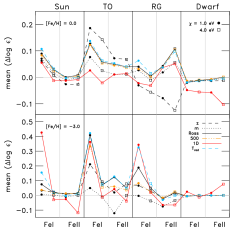
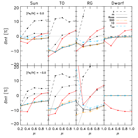
To facilitate an overall comparison between the different averages with respect to line formation, we show in Fig. 9 (left) the mean abundance deviations for weak lines that are determined between $W_{\lambda}=5-20\,\mathrm{m}\mathring{A}$. For the model representing the Sun, the differences between $\left\langle\mathrm{3D}\right\rangle$ and 3D are in general small: $\lesssim 0.1\,\mathrm{dex}$. For the TO stars at solar $\left[\mathrm{Fe}/\mathrm{H}\right]$, the differences are considerably larger: $\lesssim 0.2\,\mathrm{dex}$. We find the largest deviations for ${Fe\textsc{i}}$ lines with small excitation potential $\chi_{\mathrm{exc}}=1.0\,\mathrm{eV}$, which are the most temperature sensitive; in particular the geometrical averages exhibit strong differences. At lower metallicity, the differences increase in particular for the TO and RG model with $\lesssim 0.4\,\mathrm{dex}$, and the $\left\langle\mathrm{3D}\right\rangle$ on optical depth shows the largest deviation for metal-poor TO star. In general the deviations become smaller at higher $\chi_{\mathrm{exc}}$ and for ${Fe\textsc{ii}}$ lines. The dwarfs show very small differences compared to the full 3D case. These models exhibit the lowest velocities and temperature contrast with the mean stratifications closely resembling the 1D models based on same EOS and opacities.

The averages on column mass density $\left\langle\mathrm{3D}\right\rangle_{m}$ typically exhibit the best agreement with the predictions of the full 3D model, in particular at low metallicity. The geometrical averages $\left\langle\mathrm{3D}\right\rangle_{z}$ exhibit large deviations (in agreement with Uitenbroek & Criscuoli 2011), especially for the TO stars. When one considers the comparison of the temperature and density in Fig. 1, then one can deduce that the models with cooler stratifications are closer to the full 3D line strength. Both models averaged on constant optical depth, $\left\langle\mathrm{3D}\right\rangle_{\mathrm{Ross}}$ and $\left\langle\mathrm{3D}\right\rangle_{\mathrm{500}}$, lead to systematically larger deviations from the full 3D line formation calculations than those obtained with $\left\langle\mathrm{3D}\right\rangle_{m}$ models, in particular for low excitation ${Fe\textsc{i}}$ for the metal-poor TO star.

The resulting spectral line features with the logarithmic averages $\left\langle\mathrm{3D}\right\rangle_{\log}$ are similar to plain $\left\langle\mathrm{3D}\right\rangle_{\mathrm{Ross}}$ (therefore we refrain from showing the latter), while averages enforcing hydrostatic equilibrium, $\left\langle\mathrm{3D}\right\rangle_{\mathrm{HSE}}$, clearly fail to closely reproduce the results from 3D line formation (similar to Uitenbroek & Criscuoli 2011) and lead to rather large errors in the line formation, in particular for the metal-poor TO model (Fig. 8). Furthermore, both the flux-weighted and brightness-temperature averages, $T^{4}$ and $T_{\mathrm{rad}}$, are in general very close to the plain average, but often slightly less accurate, which is a somewhat surprising result (see $T_{\mathrm{rad}}$ in Fig. 9).

Another meaningful way to test the performance of the different averages can be accomplished by comparing the deviation of the center-to-limb variation (CLV) of the continuum intensity. In Fig. 9, we show the differences of the continuum intensity, $\delta I_{\mu}=(I_{\mu}^{\left\langle\mathrm{3D}\right\rangle}-I_{\mu}^{3\mathrm{D}})/I_{\mu}^{3\mathrm{D}}$, i.e. between the $\left\langle\mathrm{3D}\right\rangle$ and full 3D models. We find in general that the $\left\langle\mathrm{3D}\right\rangle$ models overestimate the continuum intensity at disk center ($\mu=1$), while towards the limb ($\mu=0.2$) the $\left\langle\mathrm{3D}\right\rangle$ often underestimate the intensity. The deviations of the different averages are similar to the above findings with the comparison of the curve of growth. The disk-center intensities of the 3D RHD models are matched best by the averages on column mass density $\left\langle\mathrm{3D}\right\rangle_{m}$, whereas the geometrical averages $\left\langle\mathrm{3D}\right\rangle_{z}$ display the largest discrepancies, in particular for the RG model at solar metallicity with an overestimation by $\sim 60\,\%$. The results for the averages on optical depth are once again midway between the two other kinds of averages. An interesting aspect is that the brightness-temperature averages $T_{\mathrm{rad}}$ fail to render the continuum intensities exactly, which has to be interpreted as a consequence of the non-linearity of the Planck function. Our findings are qualitatively similar to those by Uitenbroek & Criscuoli (2011).

5.3 Cautionary remarks

We remind the reader that LTE is often a very poor assumption at low $\left[\mathrm{Fe}/\mathrm{H}\right]$ (e.g. Asplund 2005) and thus that the abundance differences presented in Figs. 7 and 8 should not be added indiscriminately to results from standard 1D LTE abundance analyses. In LTE, the difference between 3D and 1D models can be very substantial for metal-poor stars for especially low excitation and minority species like ${Fe\textsc{i}}$ (e.g., Asplund et al. 1999; Collet et al. 2007), but those same lines also tend to be sensitive to departures from LTE (e.g., Bergemann et al. 2012; Lind et al. 2012) in 1D and $\left\langle\mathrm{3D}\right\rangle$ models, mainly due to overionization and overexcitation in the presence of a hotter radiation field than the local kinetic temperature (i.e., $J_{\lambda}>B_{\lambda}$). Although not explored for more than Li, one would expect that the very cool upper atmospheric layers, hence steep temperature gradients in metal-poor 3D models compared with classical 1D models, are even more prone to substantial non-LTE effects (e.g., Asplund et al. 2003; Sbordone et al. 2010). In particular, neutral species of relatively low ionization energy, such as ${Fe\textsc{i}}$, typically suffer from significant positive NLTE abundance corrections due to overionization (e.g., Asplund 2005; Bergemann et al. 2012; Lind et al. 2012) with low excitation lines are especially prone. For low-excitation ${Fe\textsc{i}}$ lines, one would therefore expect the 3D NLTE line strengths to be more similar to the 1D case than the 3D LTE results due to the positive NLTE corrections, partly compensating for the negative 3D LTE corrections. We therefore caution the reader that the 3D LTE abundance corrections presented here (3D LTE - 1D LTE) for ${Fe\textsc{i}}$ lines are likely to be too negative compared to the NLTE case (3D NLTE - 1D NLTE). As a corollary, it is inappropriate to apply a 1D NLTE abundance correction to a 3D LTE-inferred abundance when the latter is very significant, as is often the case at low $\left[\mathrm{Fe}/\mathrm{H}\right]$.

5.4 Comparison with 1D models

In Paper I we compared the $\left\langle\mathrm{3D}\right\rangle_{\mathrm{Ross}}$ stratifications with 1D models computed with the same EOS and opacity as used in the Stagger-code, in order to quantify the differences arising solely from 1D modeling based on MLT. The line formation calculations with 1D models perform quite well at solar metallicity, with the exception of the cool dwarf models (Fig. 7). However, in the metal-poor case, the lines based on the 1D models obviously do not correctly reproduce the full 3D lines by overestimating the $T$-stratifications due to the enforcement of radiative equilibrium in the upper atmosphere (Fig. 8). This is, in particular, distinctive for low-excitation neutral iron lines as previously found by Asplund et al. (1999) and Collet et al. (2007). Kučinskas et al. (2013) present similar findings for a solar-metallicity RG simulation as well, namely that neutral iron lines based on 1D MLT models are slightly closer to the full 3D lines compared to the $\left\langle\mathrm{3D}\right\rangle$ lines.

We note that in our 1D models the turbulent pressure is neglected, and the mixing length is fixed with $\alpha_{\mathrm{MLT}}=1.5$, both choices that will influence the stratification significantly. Since their effect is strongest in convective zone below the optical surface and the line formation region, the influence in terms of abundance is likely small; in fact, Kučinskas et al. (2013) only found a very small effect $<0.02\,\mathrm{dex}$ for the reduction in $\alpha_{\mathrm{MLT}}$ from 1.5 to 1.2. However, for metal-poor giants the influence can be greater for lines with very high excitation potential.

6 Conclusions

We have investigated the properties of different methods in detail for computing temporal and horizontal average stratifications from 3D RHD Stagger-grid simulations of stellar surface convection. The choice of the reference depth is critical, as comparisons of the various $\left\langle\mathrm{3D}\right\rangle$ demonstrated. We find in general that the temperature stratifications of the $\left\langle\mathrm{3D}\right\rangle_{z}$ and $\left\langle\mathrm{3D}\right\rangle_{m}$ are hotter close to the continuum forming layers and cooler in the upper layers compared to averages on surfaces of constant optical $\left\langle\mathrm{3D}\right\rangle_{\mathrm{Ross}}$ and $\left\langle\mathrm{3D}\right\rangle_{\mathrm{500}}$, while the density shows differences in the opposite sense. The flux-weighted temperature average and brightness temperature average are distinctively hotter than the plain averages, both close to the optical surface and in the upper atmosphere, since the Planck function and the fourth powers weights the larger temperatures higher. Averages obtained from the logarithmic values lead to lower temperature and density distributions by giving more weight the lower values in the distribution. These characteristics increase with higher $T_{\mathrm{eff}}$, lower $\log g$ and especially with lower $\left[\mathrm{Fe}/\mathrm{H}\right]$.

The statistical properties change depending on the reference depth scale, since the transformation to the new depth scale will inevitably imply a remapping of the values from different heights. The translation to layers of constant optical depth will smooth out temperature fluctuations as a byproduct: the temperature is in fact the main source of spatial corrugation of the surfaces of constant optical depth due to the strong temperature sensitivity of the dominant $\mathrm{H}^{-}$ continuum opacity source. Therefore, the temperature contrast and extrema are distinctively reduced, in particular in the superadiabatic region. However, this has also the side effect of enhancing both contrast and minimum-maximum range of the density. The concomitant remapping of properties from deeper or higher layers during the transformation to the new reference depth scale will in turn change the average values.

Furthermore, we examined the effects of reversed granulation in the upper layers of metal-poor stars, namely the lowering of temperatures above the granules in metal-poor 3D models compared to classical 1D models. We found that the contribution of radiative reheating due to weak spectral line absorption features relative to cooling due to mechanical expansion in the upper atmospheric layers is reduced towards higher $T_{\mathrm{eff}}$. On the other hand, the temperature in the regions immediately above the intergranular lanes are primarily controlled by mechanical expansion or compression and do not appear to be affected by the reduced metallicity. The two combined effects result in an enhanced contrast in the reversed granulation. This in turn leads to an increase in the corrugation of the surfaces of constant optical depth, which implies that the averages on constant optical depth are sampling values from a very wide range in geometrical height, thereby affecting the statistical properties such as mean value and contrast.

The comparison of ${Fe\textsc{i}}$ and ${Fe\textsc{ii}}$ calculated in full 3D and different $\left\langle\mathrm{3D}\right\rangle$ atmosphere models reveals the surprising result that the averages on column mass density $\left\langle\mathrm{3D}\right\rangle_{m}$ typically provide the best representation of the 3D model with respect to the line formation. The commonly preferred averages on layers of constant optical depth $\left\langle\mathrm{3D}\right\rangle_{\mathrm{Ross}}$ or $\left\langle\mathrm{3D}\right\rangle_{\mathrm{500}}$ in general perform worse. We located the reason for the underperformance in the predictions of 3D RHD by the $\left\langle\mathrm{3D}\right\rangle_{\tau}$ models being due to the optical depth, $d\tau_{\lambda}=\rho\kappa_{\lambda}dz$, which contains the additional non-linearity of opacity $\kappa_{\lambda}$, in contrast to the column mass density, $dm=\rho dz$; therefore, the statistical properties, in particular, the mean value, are more prone to distinctive temperature fluctuations present in the superadiabatic region and the upper layers, where the reversed granulation takes place. The differences between the lines calculated with the $\left\langle\mathrm{3D}\right\rangle_{\tau}$ models and the full 3D RHD models are significant, in particular, for metal-poor simulations due to the enhanced reversed granulation in the upper layers. We find that the neutral ${Fe\textsc{i}}$ lines with low excitation potential feature the largest differences between the mean $\left\langle\mathrm{3D}\right\rangle$ and full 3D line calculations. The 1D MLT models perform quite well at solar metallicity; however, for metal-poor models the mismatch is evident. Therefore, we caution against using 1D models for metal-poor stars, which will lead to systematic errors in the spectral analysis.

For spectral line formation calculations with $\left\langle\mathrm{3D}\right\rangle$ models from the Stagger-grid, we recommend using averages obtained on layers of constant column mass density, $\left\langle\mathrm{3D}\right\rangle_{m}$, since these provide the closest match to the spectral line strengths obtained with the full 3D RHD models. Furthermore, we advise strongly against using geometrical averages $\left\langle\mathrm{3D}\right\rangle_{z}$ for spectral line formation calculations. For purposes of improving stellar structures and asteroseismology, the $\left\langle\mathrm{3D}\right\rangle_{z}$ models are, however, useful, since these averages alone fulfill the hydrostatic equilibrium, and therefore, comparisons with helioseismological observations are in better agreement.

It is obvious that the temporally and spatially averaged models are incapable of substituting the full 3D atmospheric structure. The reduction due to the averaging will unavoidably lead to sacrificing required information. A promising intermediate approach could be the so-called "1.5D" approximation. This approach emulates atmospheric inhomogeneities, which are probed by the traversing radiation, by considering a series of perturbed 1D stratifications for spectral synthesis (e.g., see Ayres et al. 2006). In the spirit of the latter, one could utilize the temporal averaged histograms for an improved spectral line synthesis, since these contain additional information on the statistical distribution of the 3D simulations.

Appendix A Addendum to averaged models

A.1 Reversed granulation

Figure 10: Temperature contours from our model with $T_{\mathrm{eff}}=6500\,\mathrm{K}$ and $\log g=4.5$ with $\left[\mathrm{Fe}/\mathrm{H}\right]=0.0$ (left) and $-3.0$ (right). The top panels display horizontal slices with the reversed granulation pattern imprinted in the temperature map (from 3 to $7\times 10^{3}\,\mathrm{K}$) taken at $\sim 230\,\mathrm{km}$ above the surface, which is also indicated in the second panel (dashed lines). The panels below show vertical slices ($T$-contours from 2 to $17\times 10^{3}\,\mathrm{K}$) ranging from $-5.0\leq\log\tau_{\mathrm{Ross}}\leq 5.0$ on layers of constant geometrical height (second), column mass density (third) and Rosseland optical depth (last panel). These panels include isocontours of the temperature ($5,\,10$ and $12\times 10^{3}\,\mathrm{K}$; yellow lines) and density ($0.1,\,1.0$ and $2.5\times 10^{-7}\mathrm{g}/\mathrm{cm}^{3}$; blue lines) and both increase with decreasing vertical depth. We show also lines of constant optical depth (second) and geometrical depth (third and last) indicated with white lines.

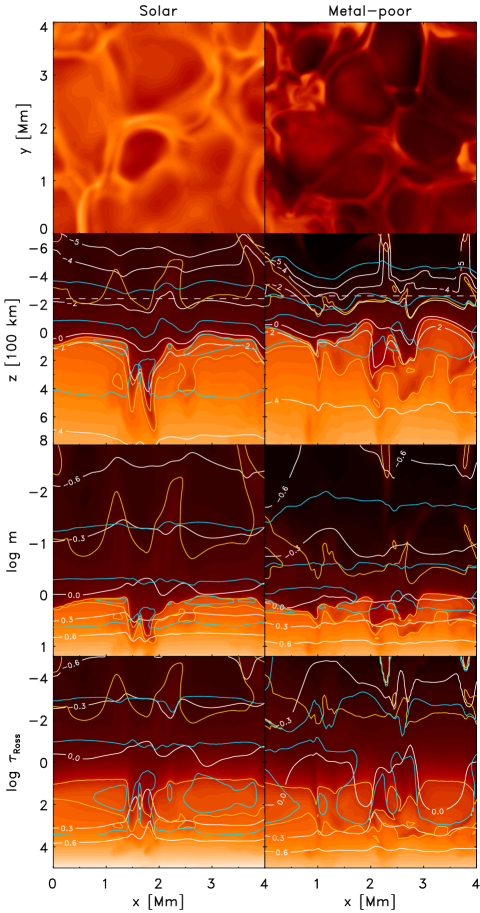
To illustrate the effects of the remapping of the 3D atmospheric structures on new reference depth scales, we show slices of temperature contours from our TO-simulation in Fig. 10. We show horizontal temperature maps taken in the upper atmosphere (top panel) and three vertical slices with different reference depth scales, which include geometrical $z$ (second panel), column mass density $m$ (third panel), and Rosseland optical depth (bottom panel). Furthermore, we indicate three different isocontours of the temperature (yellow) and density (blue lines) in Fig. 10, and we also show lines of constant optical depth $\tau_{\mathrm{Ross}}$ (white lines in top panel) or geometrical depth $z$ (middle and bottom panels).

The downdrafts just below the optical surface, which are denser and cooler than the lighter and hotter surrounding granules, are easily identified (by the prominent changes in $T,\rho$ and $\tau_{\mathrm{Ross}}$ above the downflows, e.g. $x\approx 1.8\,\mathrm{Mm}$). Owing to the lower temperatures in the downdrafts compared with the granules, the same optical depth value is reached at lower geometrical depths, meaning that the emergent radiation in the intergranular lanes originate in much deeper geometrical heights. The corrugation of the optical depth on geometrical depth scale is therefore most pronounced in the downdrafts (see isocontour of $\log\tau_{\mathrm{Ross}}=2.0$ in second panel of Fig. 10).

The opposite is true for the upper atmospheric layers because of the phenomenon of reversed granulation (Rutten et al. 2004; Cheung et al. 2007), namely, above the granules, cooling by adiabatic expansion is dominant, while above the inter granular lanes the radiative reheating and mechanical compression are more important for the energy balance. At lower metallicity and higher $T_{\mathrm{eff}}$, the radiative heating above granules is reduced by the weakening of spectral line features. The resulting reduction in radiative reheating leads to significantly cooler temperatures (see top panel in 10) and a lower pressure support, and as a consequence the atmospheric layers at a given constant optical depth subside toward lower geometrical heights, closer to the optical surface. Therefore, the temperature contrast is enhanced in the upper atmosphere. The subsiding of the atmosphere is similar to what we found earlier, namely that the density range spanned in the atmosphere is significantly reduced at lower metallicity (see Fig. 16 in Paper I). Finally, the enhancement of the reversed granulation and the temperature contrast results in strongly corrugated surfaces of constant optical depth at the top of metal-poor simulations. We note that we also found an enhanced intensity-contrast for metal-poor stars (see Paper I).

The remapping of the individual columns of the 3D structure from geometrical depth to optical depth entails a change of perspective between the old and the new scales in terms of the distribution of values of a particular physical variable at a given constant reference depth. This is again most obvious in the downdrafts in the convection zone (see line of constant geometrical depth at $z=0.2\,\mathrm{Mm}$ in bottom panel of Fig. 10). Properties from deeper geometrical heights are mapped onto layers at lower optical depth, and the temperature differences between upflowing and downflowing regions are reduced, which results in a less of a temperature contrast and in minimum-maximum ranges (see Sect. 4.1). On the other hand, the deviations in the density are significantly enhanced, which will clearly alter the statistical properties, in particular the mean values.

In the upper atmospheric layers of the solar metallicity case, the optical depth is corrugated only a small amount, therefore the transformation does not affect the temperature and density much (compare the upper flat blue line with the two lower corrugated ones in the bottom panel of Fig. 10). However, the corrugation of the optical depth in the upper atmosphere is rather large for hotter metal-poor stars owing to the enhanced reversed granulation. As a result, the effects of remapping on the optical depth scale for the temperature and density is fairly substantial in these simulations. And the distribution of the thermodynamic properties is broadened, such that the meaning of the horizontal average is weakened (see Fig. 6).

In a similar way, the translation to column mass density naturally reduces the variations in density thanks to its definition of the reference depth scale, which is the depth-integrated density. Therefore, the resulting density fluctuations are rather small in layers at constant column mass density. The variation in temperature is slightly lower than in the averages on geometrical depth, but larger than in the averages on optical depth, as one would expect.

We stress once again that the different reference depth scales are equivalent to each other in terms of the spatial remapping of the 3D atmospheric structures. What differs of course is the statistical properties of physical variables on layers of constant depth, which vary depending on the choice of reference depth scale. One has to consider two important aspects concerning the horizontal averaging, the first being what kind of quantity is considered, and the second which reference depth scale is accounted for. Therefore, the statistical properties of the density and temperature are relatively distinctive depending on which reference depth scale is considered (see Sect. 4).

A.2 Hydrostatic equilibrium

Figure 11: Deviations from the hydrostatic equilibrium vs. optical depth. Dashed lines: $\left\langle\mathrm{3D}\right\rangle_{z}$ averages; dotted lines:$\left\langle\mathrm{3D}\right\rangle_{m}$; solid lines: $\left\langle\mathrm{3D}\right\rangle_{\mathrm{Ross}}$.

The Stagger-code directly solves the discretized time-dependent, radiative-hydrodynamical equations (see Paper I) for the conservation of mass, momentum, and energy. The conservation properties are reflected in the mean $\left\langle\mathrm{3D}\right\rangle_{z}$ stratifications of relaxed, quasi-stationary 3D hydrodynamical models averaged on layers of constant geometrical depth. In particular, the geometrical averages appear over time to be close to hydrostatic equilibrium. To elucidate this further, we analyze the horizontal and time-average of the momentum equation

$$\left\langle\partial_{t}\rho\@vec{v}\right\rangle=\left\langle-\@vec{\nabla}\cdot(\rho\@vec{v}\@vec{v}+\underline{\underline{\tau}})\right\rangle-\left\langle\@vec{\nabla}p_{\mathrm{th}}\right\rangle+\left\langle\rho\@vec{g}\right\rangle$$ (4)

with $p_{\mathrm{th}}$ being the thermodynamic pressure, $\@vec{v}$ the velocity field, and $\underline{\underline{\tau}}$ the viscosity stress tensor. Due to the averaging, the only remaining spatial dependence is the vertical one. Divergence terms thus reduce to vertical derivatives, i.e., $\@vec{\nabla}\cdot\left\langle X\right\rangle=\partial_{z}\left\langle X\right\rangle$. The time derivative $\left\langle\partial_{t}\rho\@vec{v}\right\rangle$ vanishes on time average as our model atmospheres are relaxed, hence quasi-stationary. The inertial term reduces to turbulent pressure $p_{\mathrm{turb}}=\rho v_{z}^{2}$, so we obtain $\left\langle\@vec{\nabla}\cdot\left(\rho\@vec{v}\@vec{v}\right)\right\rangle=\partial_{z}\left\langle p_{\mathrm{turb}}\right\rangle$. The divergence of the viscous stress tensor, $\@vec{\nabla}\cdot\underline{\underline{\tau}}$, vanishes on average. The last two terms yield $\partial_{z}\left\langle p_{\mathrm{th}}\right\rangle$ and $\left\langle\rho g\right\rangle$, and we retrieve the equation for hydrostatic equilibrium with

$$\partial_{z}\left(\left\langle p_{\mathrm{turb}}\right\rangle+\left\langle p_{\mathrm{th}}\right\rangle\right)=-\left\langle\rho\right\rangle g.$$ (5)

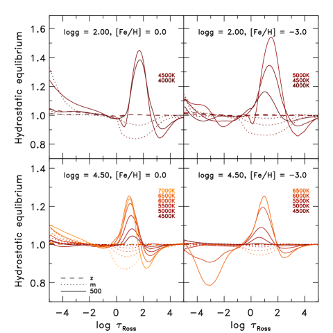
In Fig. 11 we show the hydrostatic equilibrium in the form of $\rho gdz/dp_{\mathrm{tot}}=1$ for the temporal and geometrical averaged $\left\langle\mathrm{3D}\right\rangle_{z}$ stratifications, which are very close to hydrostatic equilibrium. We emphasize that the hydrostatic equilibrium is only fulfilled by considering the total pressure $p_{\mathrm{tot}}$, as given in Eq. 5, which includes the non-thermal turbulent pressure that occupies a significant fraction of $p_{\mathrm{tot}}$ at the top and in the SAR (see Fig. 21 in Paper I).

Furthermore, one can find in Fig. 11 that the averages on a new reference depth scales feature distinctive deviations from hydrostatic equilibrium (see $\left\langle\mathrm{3D}\right\rangle_{\mathrm{Ross}}$ and $\left\langle\mathrm{3D}\right\rangle_{m}$). The transformation of to a new reference depth scale maps all three components of Eq. 5 – geometrical depth $z$, density $\rho$, and total pressure $p_{\mathrm{tot}}$ – away from its hydrostatic equilibrium state. Also, the geometrical depth $z$ loses its strict physical meaning through such a transformation as a mean value. The mean stratifications on constant Rosseland optical depth $\left\langle\mathrm{3D}\right\rangle_{\mathrm{Ross}}$ deviate slightly at the top and significantly in the SAR from the hydrostatic equilibrium ($\left\langle\mathrm{3D}\right\rangle_{\mathrm{500}}$ is very similar). The largest departures can be found in the SAR. Furthermore, the amplitude of the discrepancy from hydrostatic equilibrium increases for higher $T_{\mathrm{eff}}$ and lower $\log g$.

A.3 Deviations from the EOS

Figure 12: Deviations between the spatially and temporally averaged pressure (top) and opacity (bottom) and the values derived from the EOS, i.e. $X\left(\left\langle\rho\right\rangle,\left\langle\varepsilon\right\rangle\right)$, vs. optical depth. Dashed lines: $\left\langle\mathrm{3D}\right\rangle_{z}$ averages; dotted lines: $\left\langle\mathrm{3D}\right\rangle_{m}$; solid lines: $\left\langle\mathrm{3D}\right\rangle_{\mathrm{Ross}}$.

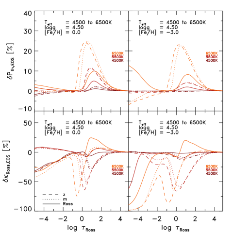
In 3D RHD simulations, the thermodynamic state of a simulation is self-consistently determined by the EOS. This means in particular that any thermodynamic variable depends on only two independent variables (namely the gas density $\rho$ and the internal energy $\varepsilon$) in a well-defined way. However, the internal self-consistency is broken by reductions like temporal or spatial averaging.

This can be easily understood by investigating the behavior of a function $f(X)$ on a 3D cube of quantity $X$. For small fluctuations $X^{\prime}=X-\left<X\right>$ around the horizontal average at a given depth in the model atmosphere, a Taylor-expansion of $f$ up to second order yields

$$f\left(X\right) = f\left(\left\langle X\right\rangle+X^{\prime}\right)$$ (6)

$$\approx f\left(\left\langle X\right\rangle\right)+\left.\frac{df}{dX}\right|_{\left\langle X\right\rangle}X^{\prime}+\left.\frac{1}{2}\frac{d^{2}f}{dX^{2}}\right|_{\left\langle X\right\rangle}X^{\prime 2}.$$ (7)

The horizontal average of this expression evaluates to

$$\left\langle f\left(X\right)\right\rangle \approx \left\langle f\left(\left\langle X\right\rangle\right)\right\rangle+\left.\frac{df}{dX}\right|_{\left\langle X\right\rangle}\left\langle X^{\prime}\right\rangle+\left.\frac{1}{2}\frac{d^{2}f}{dX^{2}}\right|_{\left\langle X\right\rangle}\left\langle X^{\prime 2}\right\rangle$$ (8)

$$= f\left(\left\langle X\right\rangle\right)+\left[\frac{1}{2}\frac{d^{2}f}{dX^{2}}\left\langle X\right\rangle^{2}\right]\delta X_{\mathrm{rms}}^{2},$$ (9)

where the definition of the contrast $\delta X_{\mathrm{rms}}$ was used in the last equation (see Eq. 3 in Sect. 4.1). The linear term in Eq. 8 vanishes as $\left\langle X^{\prime}\right\rangle=0$ by definition. It is immediately clear that $\left\langle f\left(X\right)\right\rangle=f\left(\left\langle X\right\rangle\right)$ holds for linear functions. It is thus the non-linearity of $f$ that causes a departure of $\left\langle f\left(X\right)\right\rangle$ from $f\left(\left\langle X\right\rangle\right)$, because the departure scales with the square of the contrast $\delta X_{\mathrm{rms}}$. The discussion can be easily expanded to functions of two variables $f(X,Y)$, since they are found in the EOS.

As a consequence, deriving thermodynamic quantities from averaged independent variables, $\left\langle\rho\right\rangle$ and $\left\langle\varepsilon\right\rangle$, will lead to inconsistent outcomes. The mean pressure in a given layer of the 3D cube will deviate from the pressure calculated with the EOS from mean density and mean internal energy, $\left\langle p_{\mathrm{th}}\right\rangle\not=p_{\mathrm{th}}\left(\left\langle\rho\right\rangle,\left\langle\varepsilon\right\rangle\right)$. Therefore, with $\left\langle\mathrm{3D}\right\rangle$ we face another level of complexity.

To quantify the deviations, we compute the temperature $T$, pressure $p_{\mathrm{th}}$, opacity $\kappa_{\mathrm{Ross}}$, and electron number density $n_{\mathrm{el}}$ from the EOS by employing the mean independent variables $\left\langle\rho\right\rangle$ and $\left\langle\varepsilon\right\rangle$. Then, we determine the relative disagreement as $\delta X_{\mathrm{EOS}}=(\bar{X}_{\mathrm{EOS}}-\bar{X})/\bar{X}.$ In Fig. 12, we display the deviations of thermal pressure $\delta p_{\mathrm{th}}^{\mathrm{EOS}}$ and opacity $\delta\kappa_{\mathrm{Ross}}^{\mathrm{EOS}}$. As suggested by Eq. 9, we find the maximal deviations typically below the optical surface in the SAR, where the large fluctuations take place due to the overturning and to the presence of convective motions with their highly asymmetric up and downflows. The mean value thus toddles between the bimodal distribution. Furthermore, we find a strong variation in the $\delta X_{\mathrm{EOS}}$ with stellar parameter, which increases for higher $T_{\mathrm{eff}}$ and lower $\log g$. Depending on which reference depth scale is applied, the disagreement $\delta X_{\mathrm{EOS}}$ are distinct.

This loss of consistency caused by dimensional reduction means that mean $\left\langle\mathrm{3D}\right\rangle$ models can never entirely substitute full 3D models, especially for spectral line formation applications (Uitenbroek & Criscuoli 2011). The mean stratifications are nothing more than statistically meaningful representations of stellar atmospheres, while only the complete 3D data set describes their physical state completely. In 1D model atmospheres, such internal consistency is maintained at all times, since no spatial averaging of non-linear variables is involved in the construction of 1D models.