Novel Linear Algebraic Theory and One-hundred-million-atom Electronic Structure Calculation on The K Computer

Abstract

A novel linear-algebraic algorithm, multiple Arnoldi method, was developed in an interdisciplinary study between physics and applied mathematics and realized one-hundred-million-atom (100-nm-scale) electronic state calculations on the K computer. The algorithms are Krylov-subspace solvers for generalized shifted linear equations and were implemented in our order-$N$ calculation code ELSES (http://www.elses.jp/). Moreover, a method for calculating eigen states is presented as a theoretical extension.

1 Introduction

Large scale electronic structure calculation, with thousand atoms or more, is of great importance both in science and technology. Recently, calculations with ten million atoms were realized on the K computer [1, 2] by our code ELSES (http://www.elses.jp/). The computational cost is order-$N$ or is proportional to the number of atoms $N$, as shown in Fig. 3(a) of Ref. [1]. The present paper presents more recent calculations for larger systems with one hundred million atoms and the calculations are called ‘100-nm-scale calculation’, because one hundred million atoms are those in silicon single crystal with the volume of $V=$(126nm)³. The present paper also presents a calculation method of specific eigen states with a polymer example. The calculation was carried out with modeled (tight-binding) electronic structure theory based on ab initio calculations. The detailed theory is described in Ref. [1]

2 Method and parallel efficiency

The used linear algebraic method is called multiple Arnoldi (mArnoldi) method. [1] The mathematical foundation is the ‘generalized shifted linear equation’, or the set of linear equations

$$(zS-H)\bm{x}=\bm{b},$$ (1)

where $z$ is a (complex) energy value and $H$ and $S$ denote the Hamiltonian and overlap matrices in the linear-combination-of-atomic-orbital (LCAO) representation, respectively. The matrices are sparse real-symmetric $M\times M$ matrices, and $S$ is positive definite. The vector $\bm{b}$ is the input and the vector $\bm{x}$ is the solution vector. Equation (1) is solved, instead of the original generalized eigen-value equation

$$H\bm{\phi}_{k}=\varepsilon_{k}S\bm{\phi}_{k}.$$ (2)

The method is purely mathematical and may be applicable to other problems.

The mArnoldi method [1] reduces the problem into a set of many small $(\nu\times\nu)$ standard eigen-value equations defined within the Krylov sub(Hilbert)spaces of $\{{\cal L}_{\nu}^{(j)}\}$, where $j$ is the basis index $(j=1,2,3,....M)$ and $\nu$ is the subspace dimension typically $\nu=30-300$. The $j$-th subspace (${\cal L}_{\nu}^{(j)}$) contains the $j$-th unit vector of $\bm{e}_{j}\equiv(0,0,..1_{j},0,.,0_{M})^{\rm t}$ ($\bm{e}_{j}\in{\cal L}_{\nu}^{(j)}$). For each subspace eigen-value equation, eigen levels $\{\varepsilon^{(j)}_{\alpha}\}$ and eigen vectors $\{\bm{v}^{(j)}_{\alpha}\}$ ($\alpha=1,2,..,\nu$) are obtained and are called subspace eigen levels and subspace eigen vectors, respectively. The Green’s function is determined by the subspace eigen levels and vectors and gives the total energy and force.

Figure 1(a) shows the parallel efficiency on the K computer with one hundred million atoms ($N=$103,219,200). The elapse time $T$ is measured as the function of the number of used processor cores $P$ $(T=T(P))$, where $P=P_{\rm min}\equiv 32,768$, $P_{a}\equiv$98,304, $P_{b}\equiv$294,912, $P_{\rm all}\equiv 663,552$ (all cores). The resultant benchmark is called ‘strong scaling’ in the high-performance computation society. The calculated material is sp²-sp³ nano-composite carbon solid. [2] The time of the total energy calculation was measured for a given atomic structure. The measured parallel efficiency, $\alpha(P)\equiv T(P)/T(P_{\rm min})$, was $\alpha(P_{a})=0.98$, $\alpha(P_{b})=0.90$ and $\alpha(P_{\rm all})=0.73$.

Figure 1: (a) Parallel efficiency on the K computer with $N=$103,219,200 atoms. The calculations were carried out with the total number of processor cores $P$ = 32,768, 98,304, 294,912, 663,552 (all cores). The calculated material is sp²-sp³ nano-composite carbon solid. (b) Structure of poly-(9,9 dioctyl-fluorene). Here $R\equiv$ C₈H₁₇. (c) A molecular dynamics simulation of a poly-(9,9 dioctyl-fluorene) system.

3 Method for calculating eigen states

This section is devoted to a calculation method for individual eigen states in the mArnoldi method, since it is missing in our previous papers. [1, 2] A conjugated polymer system depicted in Figs. 1(b)(c), poly-(9,9 dioctyl-fluorene), was chosen as a test system. The poly-fluorene and its family are famous as a hopeful candidate for industrial lighting applications. A previous theoretical paper [3] investigates related small molecules and drove us to calculations of polymer materials with non-ideal (amorphous-like) structures. The present calculations are intended for a methodological test, in particular, on $\pi$ states. As a reference data, the monomer and dimer were calculated by the present method and the ab initio calculation of Gaussian^(TM) and the results agree reasonably among the two methods. [1] The calculated highest-occupied (HO) and lowest-unoccupied (LU) states of dimer are contributed only by the $\pi$ states of benzene rings, as in benzene, and are illustrated in Fig.2(a) and (b), respectively. A molecular dynamics simulation with 2076 atoms was carried out as shown in Fig. 1(c). An artificially packed structure was thermally relaxed within the period of $T$=80 ps, so as to obtain non-ideal polymer structures.  [1] The calculated DOS is shown in Fig.2 of Ref. [1]. Hereafter the same poly-fluorene system will be discussed in the same calculation conditions as in the DOS.

The method for calculating the $k$-th eigen level ($\varepsilon_{k}$) and vector ($\bm{\phi}_{k}$) are explained; The Green’s function gives the integrated density of states $n=n(\eta)$ and its inverse function $\eta=\eta(n)$. The $k$-th eigen level is determined in the inner product form of $\varepsilon_{k}:=\eta(k-1/2)$ (See Footnote 9 of Ref. [1]). Then, the $k$-th eigen vector ($\bm{\phi}_{k}$) is calculated from the subspace eigen vectors of which energy levels lie in the range of $\eta(k-1)<\varepsilon<\eta(k)$ so that the $j$-th component $(\bm{e}_{j}^{\rm t}\bm{\phi}_{k})$ is determined as

$$\bm{e}_{j}^{\rm t}\bm{\phi}_{k}:=\sum_{\alpha}\bm{e}_{j}^{\rm t}\bm{v}_{\alpha}^{(j)}\int_{\eta(k-1)}^{\eta(k)}\delta(\varepsilon-\varepsilon_{\alpha}^{(j)})d\varepsilon.$$ (3)

Here the delta function in the above equation is a ‘smoothed’ one. Additional techniques for calculating eigen vectors are given in in Appendix.

Figure 2(c) is a part of the polymer system at which the calculated HO and LU wavefunctions are localized, as in Figs 2(d) and (e), respectively. They are $\pi$ states and two features are found; (I) The characteristic node structures are observed and are the same as in the dimer case (Fig. 2(a) and (b)). In short, the HO and LU wavefunctions of the polymer are connected HO and LU wavefunctions of dimer, respectively. (II) The wavefunctions are localized on the chain structure among four monomers and terminated at one inter-monomer boundary indicated by an arrow. At that boundary, the structure is largely tilted (or twisted) and the $\pi$ states are disconnected. There features are confirmed in the wavefunctions given by the exact diagonalization method.

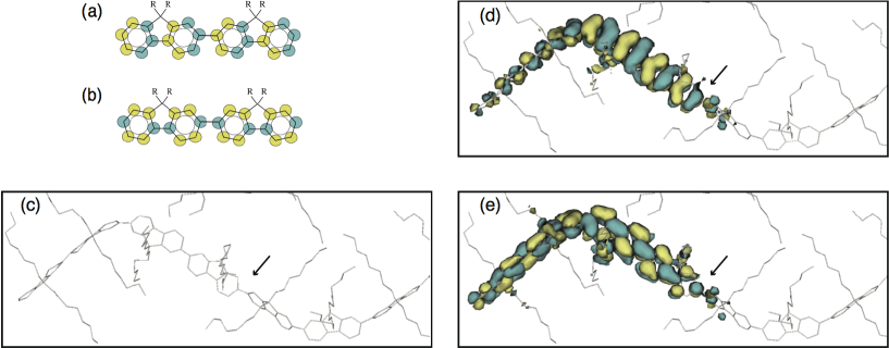
Figure 2: (a)(b) Schematic figures of the HO or LO ($\pi$) state of fluorene dimer, respectively. (c)-(e) A part of the poly-fluorene system is shown in (c) and the calculated HO and LU wavefunctions are shown in (d) and (e), respectively. Only carbon atoms and carbon-carbon bonds are drawn.

4 Summary and future outlook

The present paper shows methods and results of one-hundred-atom electronic structure calculations based on our novel linear algebraic algorithm. For future outlook, methods for automatic determination of model (tight-binding) parameters are developing, [4] so as to enhance studies of various materials. Matrix data $(H,S)$ for materials [5] and a small application for matrix solvers [6] are prepared for further interdisciplinary study between physics and applied mathematics.

Acknowledgments     This research is partially supported by Grant-in-Aid for Scientific Research (Nos. 23540370 and 25104718) from the MEXT of Japan. The K computer was used in the research proposals of hp120170 and hp120280. Supercomputers were also used at the Institute for Solid State Physics, University of Tokyo, at the Research Center for Computational Science, Okazaki, and at the Information Technology Center, University of Tokyo. The authors thank Y. Zempo (Hosei University) and M. Ishida (Sumitomo Chemical Co., Ltd) for providing the structure model of poly-fluorene system. The wavefunctions in Figs. 2(d)(e) are drawn by an original python-based visualization tool VisBAR_wave_batch, a part of VisBAR package. [2]

Appendix A Refinement techniques for specific eigen vectors

Refinement techniques for a specific eigen vector ($\bm{\phi}$) is explained, where the level index ($k$) is discarded. A subspace eigen vector ($\bm{v}_{\alpha}^{(j)}$) has the sign-flipping freedom ($\bm{v}_{\alpha}^{(j)}\Rightarrow-\bm{v}_{\alpha}^{(j)}$) and the correct sign should be assigned. In the code, a ‘reference’ subspace eigen vector, denoted as $\bm{v}_{{\rm ref}}$, is chosen among the subspace eigen vectors ({ $\bm{v}_{\alpha}^{(j)}$ }) so that the ‘reference’ subspace eigen vector has the largest weight contribution to the eigen vector $\bm{\phi}$. The sign of a subspace eigen vectors ($\bm{v}_{\alpha}^{(j)}$) in Eq. (3) is determined so that the inner product between $\bm{v}_{{\rm ref}}$ and $\bm{v}_{\alpha}^{(j)}$ is positive ($\bm{v}_{{\rm ref}}^{\rm t}\bm{v}_{\alpha}^{(j)}>0$). If the subspace eigen vectors are exact, the above procedure gives the correct sign of wavefuction. Since this method, called inner product method, is insufficient in several cases, a further refinement technique, called local flipping method’, is used. The target eigen level and vector are denoted as $\varepsilon$, and $\bm{\phi}\equiv(a_{1},a_{2},.....a_{M})^{\rm t}$. The method gives an iterative local sign flipping processes $(a_{l}\Rightarrow-a_{l})$, so as to reduce the residual norm ${\cal R}\equiv\bm{r}^{\rm t}\bm{r}$ defined by the residual vector of $\bm{r}\equiv(H-\varepsilon S)\bm{\phi}$. The details will appear elsewhere. As an additional technique for faster convergence, the LU state $\bm{\phi}$ (Fig. 2(e)) was calculated after the calculation of the HO state $\bm{\phi}_{\rm HO}$ (Fig. 2(d)) with the redefinition of the residual norm $R$ as ${\cal R}\equiv\bm{r}^{\rm t}\bm{r}+c\,|\bm{\phi}_{\rm HO}^{\rm t}S\bm{\phi}|^{2}$ with a positive parameter $c$(=5a.u.). The minimization of the additional term is an effective orthogonality constraint $(|\bm{\phi}_{\rm HO}^{\rm t}S\bm{\phi}|\rightarrow 0)$. The wavefunctions in Fig. 2(d)(e) are obtained after $10^{1}$-$10^{2}$ local sign flipping iterates. The above sign flipping procedure consumes only a small computational cost, since no matrix-vector multiplication is required. A further refinement can be achieved by another method, such as Jacobi-Davidson method [7], though it requires matrix-vector multiplications.

References

- [1] T. Hoshi, S. Yamamoto, T. Fujiwara, T. Sogabe, S.-L. Zhang: J. Phys.: Condens. Matter 21 (2012) 165502.
- [2] T. Hoshi, Y. Akiyama, T. Tanaka and T. Ohno: J. Phys. Soc. Jpn. 82 (2013) 023710.
- [3] Y. Zempo, N. Akino, M. Ishida, M. Ishitobi and Y. Kurita, J. Phys.: Condens. Matter 20 (2008) 064231.
- [4] S. Nishino, T. Fujiwara, H. Yamasaki, S. Yamamoto, T. Hoshi, Solid State Ionics 225 (2012) 22–25; Y. Ohtani, T. Fujiwara, S. Nishino, T. Suzuki, S. Yamamoto and Y. Zempo, MRS Proceedings 1523 (2013) QQ6-08; S. Nishino and T. Fujiwara J. Mol. Model. 19 (2013) 2363.
- [5] ELSES matrix library: http://www.elses.jp/matrix/
- [6] Eigen Test: http://www.damp.tottori-u.ac.jp/~hoshi/eigen_test/
- [7] See textbooks, such as, Z. Bai, J. Demmel, J. Dongrarra, A. Ruhe, and H. van der Vorst, Templates for the Solution of Algebraic Eigenvalue Problems, SIAM, Philadelphia, (2000).