Yield stress in amorphous solids: A mode-coupling theory analysis

Abstract

The yield stress is a defining feature of amorphous materials which is difficult to analyze theoretically, because it stems from the strongly non-linear response of an arrested solid to an applied deformation. Mode-coupling theory predicts the flow curves of materials undergoing a glass transition, and thus offers predictions for the yield stress of amorphous solids. We use this approach to analyse several classes of disordered solids, using simple models of hard sphere glasses, soft glasses, and metallic glasses for which the mode-coupling predictions can be directly compared to the outcome of numerical measurements. The theory correctly describes the emergence of a yield stress of entropic nature in hard sphere glasses, and its rapid growth as density approaches random close packing at qualitative level. By contrast, the emergence of solid behaviour in soft and metallic glasses, which originates from direct particle interactions is not well described by the theory. We show that similar shortcomings arise in the description of the vibrational dynamics of the glass phase at rest. We discuss the range of applicability of mode-coupling theory to understand the yield stress and non-linear rheology of amorphous materials.

I Introduction

The yield stress is a defining characteristics of amorphous solids which represents a robust mechanical signature of the emergence of solid behaviour in many atomic, molecular and soft condensed materials undergoing a transition between fluid and solid states barnes ; coussot2 . From a physical viewpoint, the existence of a yield stress implies that the material does not flow spontaneously unless a driving force of finite amplitude is applied, which represents a very intuitive definition of ‘solidity’. While properly defining and measuring a yield stress remains a debated experimental issue bonn , we will study simple model systems where the yield stress can be unambiguously identified as the shear stress $\sigma$ measured in steady state shear flow, in the limit where the deformation rate $\dot{\gamma}$ goes to zero,

$$\sigma_{Y}=\lim_{\dot{\gamma}\to 0}\sigma(\dot{\gamma}).$$ (1)

As such, the yield stress measures a strongly nonlinear transition point between flowing states for $\sigma>\sigma_{Y}$ and arrested states when $\sigma<\sigma_{Y}$. In this work, we wish to analyze the dependence of $\sigma_{Y}$ upon external control parameters, such as temperature $T$, packing fraction, $\varphi$, in a wide range of disordered materials. Therefore, our work differs from most rheological studies of glassy materials which usually describe a set of flow curves, $\sigma=\sigma(\dot{\gamma})$, for a specific material.

Dense amorphous particle packings represent a broad class of solids possessing a yield stress, which typically emerges when either temperature is lowered across the glass transition temperature $T_{g}$ in atomic and molecular glasses (such as metallic glasses), or when the packing fraction is increased in colloidal hard spheres and soft glassy materials (such as emulsions and soft colloidal suspensions) binder ; rmp . Of course, the range of materials displaying a measurable yield stress is much broader barnes , but we restrict ourselves to dense particle systems with a disordered, homogeneous structure, leaving aside systems like colloidal gels or crystalline and polycrystalline structures.

While our emphasis is mostly on atomic and colloidal systems, we also include in our discussion materials such as foams and noncolloidal soft suspensions, where solidity emerges upon compression at the jamming transition, but for which thermal fluctuations play a negligible role reviewmodes . While the yield stress in jammed solids results from the emergence of a mechanically stable contact network between particles rather than a glass transition vhjpcm , it was recently demonstrated that the interplay between glass and jamming transitions can be experimentally relevant for the rheology of soft colloidal systems as well ikeda . In particular, we have shown that the yield stress of soft repulsive particles displays a very rich behaviour as both $T$ and $\varphi$ are varied ikeda , and we suggested that this is relevant to describe materials such as concentrated emulsions softmatter (see also Ref. mason ).

From the modelling point of view, the complex rheology of amorphous yield stress materials is often described using simplified or coarse-grained descriptions that assume from the start the existence of a yield stress, and study the response of the solid to the imposed flow picard ; vdb ; jagla ; kirsten1 ; bocquet . Fewer theoretical approaches can describe both the emergence of a yield stress together with the rheological consequences sgr ; hb ; BBK , as they must then also in principle provide a faithful description of the glass or jamming transitions, which represent theoretical challenges on their own rmp . Therefore it should be clear that predicting the temperature and density evolution of the yield stress across a broad range of materials is much more demanding than studying the qualitative evolution of a set of flow curves. Thus, we hope our study will motivate further theoretical developments to reach this goal.

The mode-coupling theory (MCT) of the glass transition was first developed in the context of the statistical mechanics of the liquid state to account for the dynamical slowing down observed in simple fluids approaching the glass transition gotze , but it has also deep connections to the random first order transition theory of the same problem, that are well understood rmp . While initially thought as a theory for the glass transition, it is now recognized that MCT can make relevant predictions for time correlation functions for the initial 2-3 decades of viscous slowing down. Interestingly, this time window is very relevant for experiments performed in colloidal systems and in computer simulation studies. This explains why the theory continues to be developed as of today, and in particular why its extensions to account for the driven dynamics of glasses have experimental relevance kuni1 ; kuni2 ; fuchs1 ; fuchs2 ; fuchs3 . Many specific aspects of the theory have received numerical and experimental attention in recent years kuni2 ; fuchs4 , but a systematic exploration of the yield stress behaviour has, to our knowledge, not been performed.

To explore different types of materials while keeping the possibility of a direct comparison to theorical predictions, we concentrate on simple model systems which can be both efficiently studied in computer simulations to obtain direct measurements of the yield stress, and can also be studied within a mode-coupling approach. Because the static structure of the fluid is the only input needed for the theory, measuring the structure from computer simulations nauroth ; gillesmct allows us to directly analyse the validity of the theoretical predictions, and identify precisely the strength, weakness and range of applicability of the theory to analyze the yield stress of amorphous solids.

In agreement with previous findings, we observe that for all systems, the theory correctly predicts the emergence of a finite yield stress as the glass transition is crossed, although it is difficult to assess quantitatively the detailed predictions made by the theory near the ‘critical’ point (because the singularity is replaced by a crossover in real systems). For hard sphere glasses, the theory accounts qualitatively well for both the entropic nature of the solidity (i.e., $\sigma_{Y}\propto k_{B}T$) and the divergence of the yield stress as the random close packing density is approached mewis . By contrast, we find that the theory fares poorly for systems where solidity emerges due direct interparticle interactions (i.e., $\sigma_{Y}\propto\epsilon$, where $\epsilon$ characterizes the scale of pair interactions) such as soft repulsive and Lennard-Jones particles at low temperatures, as theory incorrectly predicts that $\sigma_{Y}\sim k_{B}T$. Our results also show that these shortcomings can be traced back to the description of the glass dynamics at rest (i.e. without an imposed shear flow), rather than to an incorrect treatment of the mechanical driving. Therefore, we also offer a detailed analysis of the vibrational dynamics in all these models, which is currently the focus of considerable attention, in particular in colloidal materials bonnmode ; soft ; criticality .

The paper is organized as follows. In Sec. II we introduce our models for hard spheres, soft and metallic glasses, and the mode-coupling approach we follow to study the glass dynamics at rest and under flow. In Sec. III we study the vibrational glass dynamics of hard sphere and soft sphere glasses at rest. In Sec. IV we study the glassy rheology of hard sphere and soft sphere models. In Sec. V we repeat the analysis of vibrational and rheological properties for Lennard-Jones particles. In Sec. VI we discuss our results and offer perspectives for future research.

II Models, methods and mode-coupling theory

In this section we introduce the models used to describe the physics of hard spheres, soft and metallic glasses. Then, we describe the simulation methods employed to extract vibrational dynamics and the yield stress. Finally we present the mode-coupling theory to analyse both the glass dynamics at rest and its extension to treat steady state shear flows.

II.1 Model glasses

In this work, we consider two different model systems. To address the physics of hard spheres and soft glasses we study a system of repulsive harmonic spheres, defined by the simple following pairwise potential,

$$v_{HS}(r_{ij})=\frac{\epsilon}{2}(1-r_{ij}/a)^{2}\Theta(a-r_{ij}),$$ (2)

where $\Theta(x)$ is the Heaviside function and $a$ is the particle diameter.

It is well established that harmonic spheres display two different regimes when the packing fraction, $\varphi$, and temperature, $T$, are varied tom . Because of the repulsive interaction, harmonic spheres at low temperatures have very few overlaps and thus effectively behave, in the limit of $\epsilon/T\to\infty$ as a hard sphere fluid. In this regime, the physics of harmonic spheres is controlled by entropic forces. However, this regime can only be achieved if the density is low enough that configurations with no particle overlap can easily be found. Upon compression, another regime is entered where particles have significant overlaps with their neighbors, and the system then behaves as a soft repulsive glass. In this regime, the physics is controlled by the energy scale $\epsilon$ of the repulsive forces rather than by entropic forces. At very low temperatures, the transition between these two distinct glasses occurs at the jamming transition ohern1 . In this paper, our primary goal is not to study the jamming transition in detail, but rather to use its existence to study both the ‘entropic’ physics of hard spheres and the ‘energetic’ physics of soft glasses within a single model.

Finally, we use Lennard-Jones particles as a simple model for an atomic glass-forming liquid, where the pairwise potential is

$$v_{LJ}(r_{ij})=4\epsilon\left((a/r_{ij})^{12}-(a/r_{ij})^{6}\right).$$ (3)

As we mainly deal with the properties of the glass we use a monodisperse Lennard-Jones model. To study also the viscous liquid properties, we would need to study a system with some size polydispersity (such as a binary mixture) to prevent crystallization. Such mixtures are indeed taken as simple models for metallic glasses. In this case again, the energy scale $\epsilon$ in the Lennard-Jones potential plays a crucial role, as we shall demonstrate.

II.2 Computer simulations

To assess the quality of the mode-coupling theory predictions we have studied the above models using computer simulations, both by producing new data for the present work, and by collecting previously published data. The simulation methods are described in our previous publications ikeda ; criticality ; LJ , and so we only give a brief account of these methods.

To study the vibrational dynamics of the various glass structures, we performed Newtonian dynamics simulations. We studied the vibrational property of a single amorphous packing configuration at the desired density and temperature, using a very large system size criticality . To generate the glass configurations, we first prepare a fully random configurations, and then perform an instantaneous quench to very low temperature. We then let the system relax until aging effects become negligible, and purely vibrational dynamics is observed. To study glasses at different state points, we heat or cool, we compress or decompress the initially prepared glass configuration, followed by a new thermalization. After the glass structures are obtained, we perform production runs. Since we mainly focus on the very low temperatures (compared to the glass transition temperature), the system lies well inside a metastable state, and particles simply perform vibrational motions around their equilibrium positions.

For numerical simulations of the yield stress of the harmonic sphere system, we performed Langevin dynamics simulations with simple shear flow ikeda . The equation of motion is

$$\xi(\frac{\partial\vec{r}_{i}}{\partial t}-\dot{\gamma}y_{i}\vec{e}_{x})=-\sum_{j=1}^{N}\frac{\partial v(|\vec{r}_{i}-\vec{r}_{j}|)}{\partial\vec{r}_{i}}+\vec{R}_{i}.$$ (4)

Here $\vec{r}_{i}$ represents the position of particle $i$, $y_{i}$ its $y$-component, and $\vec{e}_{x}$ the unit vector along the $x$-axis. The damping coefficient, $\xi$, and the random force, $\vec{R}_{i}(t)$, obey the fluctuation-dissipation relation: $\langle{\vec{R}_{i,\alpha}(s)\vec{R}_{j,\beta}(s^{\prime})}\rangle=2k_{B}T\xi\delta_{ij}\delta_{\alpha\beta}\delta(s-s^{\prime})$. We apply Lees-Edwards periodic boundary conditions. We performed sufficiently long simulations at the desired temperature, density and shear rate, and analyzed their steady state stress measured via the standard Irving-Kirkwood formula. The yield stress is typically extracted from fitting the steady state flow curves at a given state point using a phenomenological Herschel-Bulkley law, $\sigma(\dot{\gamma})=\sigma_{Y}+a\dot{\gamma}^{n}$, where $a$ and $n$ are additional fitted parameters.

Because the yield stress of the Lennard-Jones model has been measured in a number of studies for the case of a well-known binary mixture yieldLJ ; yieldLJ2 , we gather these literature data as a proxy for the yield stress of the monocomponent system. Since our discussion of these data is mainly qualitative, the differences between both systems have no impact for the present work.

For both harmonic and Lennard-Jones spheres, we use $a$ and $\epsilon/k_{B}$ as the units of the length and temperature. For the time unit, $a(m/\epsilon)^{1/2}$ and $a^{2}\xi/k_{B}T$ are used in the inertial dynamics (for vibration) and overdamped dynamics (for rheology), respectively, where $m$ is the particle mass. We will carefully discuss the appropriate stress scales when needed.

II.3 Mode-coupling theory (MCT) of the glass transition

We present the basic mode-coupling equations allowing us to describe the dynamics of glassy liquids and glasses at rest. The mode-coupling theory (MCT) gotze of the glass transition can be expressed as a closed set of equations for the intermediate scattering functions $F(\vec{k},t)=N^{-1}\langle{\rho(\vec{k},0)^{*}\rho(\vec{k},t)}\rangle$. Here, $\rho(\vec{k},t)=\sum_{i}e^{i\vec{k}\cdot\vec{R}_{i}(t)}$ is the instantaneous density field and $\vec{R}_{i}(t)$ is the $i$-th particle position at time $t$. The central equation of the MCT is

$$\begin{aligned} \Omega^{-2}(k)\ddot{F}(k,t)+F(k,t)+\int^{t}_{0}\!\!ds\ M(k,t-s)\dot{F}(k,s)=0,\end{aligned}$$ (5)

where $\Omega(k)=\sqrt{k_{B}Tk^{2}/mS(k)}$ is the frequency term associated with acoustic waves, and $S(k)=F(k,t=0)$ is the static structure factor. The memory kernel $M(k,t)$ is given by

$$\begin{aligned} M(k,t)=\frac{\rho S(k)}{2k^{2}}\int\!\!\frac{d\vec{q}}{(2\pi)^{3}}V(\vec{k},\vec{q},\vec{k}-\vec{q})F(q,t)F(|\vec{k}-\vec{q}|,t),\end{aligned}$$ (6)

with the vertex term

$$\begin{aligned} V(\vec{k},\vec{q},\vec{p})=\{\vec{k}\cdot\vec{q}c(q)+\vec{k}\cdot\vec{p}c(p)\}^{2}/k^{2}.\end{aligned}$$ (7)

Here, $c(k)=\{1-1/S(k)\}/\rho$ is the direct correlation function hansen .

From the intermediate scattering function, we can also obtain various incoherent correlation functions in the framework of the MCT. Consider a tagged particle located at $\vec{R}(t)$, and the associated density field $\rho_{s}(\vec{k},t)=e^{i\vec{k}\cdot\vec{R}(t)}$. The MCT equations for the self intermediate scattering function $F_{s}(k,t)=\langle{\rho_{s}(\vec{k},0)^{*}\rho_{s}(\vec{k},t)}\rangle$ have the same structure as Eq. (5), but with the frequency term now given by $\Omega_{s}(k)=\sqrt{k_{B}Tk^{2}/m}$ instead of $\Omega(k)$, and with the self memory kernel

$$M_{s}(k,t)\!=\!\frac{\rho}{k^{2}}\!\int\!\!\frac{d\vec{q}}{(2\pi)^{3}}\left\{\!\frac{\vec{k}\cdot\vec{q}}{k}c(q)\!\right\}^{2}\!\!F_{s}(q,t)F(|\vec{k}-\vec{q}|,t),$$ (8)

instead of $M(k,t)$. The MCT equation for the mean-squared displacement, $\Delta^{2}(t)=\langle{|\vec{R}(t)-\vec{R}(0)|^{2}}\rangle$, can also be obtained:

$$\begin{aligned} \frac{m}{k_{B}T}\ddot{\Delta}^{2}(t)-6+\int^{t}_{0}\!\!ds\ M_{d}(t-s)\dot{\Delta}^{2}(s)=0,\end{aligned}$$ (9)

where

$$M_{d}(t)\!=\!\frac{\rho}{6\pi^{2}}\!\int\!\!dk\ k^{4}c(k)^{2}F(k,t)F_{s}(k,t).$$ (10)

The set of MCT equations describes the time evolution of the correlation functions $F(k,t)$, $F_{s}(k,t)$, and $\Delta^{2}(t)$. The MCT equations have been applied to various model systems including the two models studied in this work, harmonic spheres and Lennard-Jones particles nauroth ; beng ; gillesmct ; harmmct . In both cases, the theory predicts an ideal glass transition line in the $(T,\varphi)$ phase diagram. At high temperature and low densities, $F(k,t)$ and $F_{s}(k,t)$ relax to zero and $\Delta^{2}(t)$ becomes diffusive, $\Delta^{2}(t)\propto t$, at long time. However when the temperature is decreased and the density is increased, the system may enter the non-ergodic glass phase, where the long time limits of $F(k,t)$ and $F_{s}(k,t)$ are positive, and the limit of $\Delta^{2}(t)$ is finite.

To characterize vibrational dynamics in the glass phase, we focus on the mean-squared displacement $\Delta^{2}(t)$. We compare $\Delta^{2}(t)$ obtained from MCT with the direct numerical measurements. Since the MCT equation of the mean squared displacement Eqs. (9) and  (10) depend on the collective and self intermediate scattering functions, we first need to solve the full MCT equations Eq. (5) for these correlation functions. This requires the static structure factor $S(k)$ as a sole input. We use the ‘exact’ $S(k)$ directly obtained from the simulations at each state point. For the numerical integration of Eqs. (6), (8), and (10), we employed equally spaced grids $N_{k}$ with a grid spacing $\Delta k$. We use large enough $N_{k}\Delta k$ and small enough $\Delta k$ to be independent from the choice of these parameters.

Integrating the MCT equations for very low $T$ very close to the jamming transition for harmonic spheres required an usually large number of wavevectors $N_{k}$, as the static structure develops singularities. We made sure that all our results are well converged and depend only weakly on the numerical integration. We discuss this issue in more detail in Sec. III.3.1.

II.4 Mode-coupling theory under shear flow

In the past decade, the mode-coupling theory of the glass transition has been extended to study systems under shear flow kuni1 ; kuni2 ; fuchs1 ; fuchs2 . In this work, we follow the approach developed in Refs. fuchs1 ; fuchs2 . The theory describes a system that is subjected to shear flow at $t=0$, and predicts how the system reaches a steady state. As before, it only requires the static structure factor at rest as an input, and gives properties of the steady state under shear flow as output, from which we can deduce the value of the yield stress.

The theory again takes the form of a closed set of equations for the transient intermediate scattering function, $F_{t}(\vec{k},t)\equiv\langle{\rho(\vec{k},0)^{*}\rho(\vec{k}(t),t)}\rangle$. This function is the extension of $F(k,t)$ to describe the transient dynamics of the system, where the shear flow is applied at $t=0$. The so-called advected wave vector $\vec{k}(t)$ is given by $\vec{k}(t)=\vec{k}-\dot{\gamma}k_{x}\vec{e}_{y}t$, which takes into account the affine advection of density fluctuations by the shear flow. The central equation of the theory is very similar to the usual MCT equation, Eq. (5), except that the transient correlation function becomes the unknown function. In practice, however, the equations become very difficult to solve because the correlation functions are anisotropic, due to the external flow, and we cannot perform the circular integral before solving the equations.

To avoid this problem, we employ the approximation called ‘isotropically sheared model’ fuchs1 , where an isotropic approximation is applied to all correlation functions and advected wavevectors. In this approximation, the central equation is

$$\begin{aligned} \Gamma^{-1}(k)\dot{F}_{t}(k,t)+F_{t}(k,t)+\int^{t}_{0}\!\!ds\ M_{t}(k,t-s)\dot{F}_{t}(k,s)=0,\end{aligned}$$ (11)

where $\Gamma(k)=k_{B}Tk^{2}/\xi S(k)$ is the damping term and $M_{t}(k,t)$ is the memory kernel given by:

$$\begin{aligned} M_{t}(k,t)=\frac{\rho S(k)}{2k^{2}}\int\!\!\frac{d\vec{q}}{(2\pi)^{3}}V_{t}(\vec{k},\vec{q},\vec{k}-\vec{q},t)F_{t}(q,t)F_{t}(|\vec{k}-\vec{q}|,t),\end{aligned}$$ (12)

with the vertex term

$$\begin{aligned} V_{t}(\vec{k},\vec{q},\vec{p},t)=\{\vec{k}\cdot\vec{q}c(q)+\vec{k}\cdot\vec{p}c(p)\}\\ \{\vec{k}\cdot\vec{q}c(q(t))+\vec{k}\cdot\vec{p}c(p(t))\}/k^{2}.\end{aligned}$$ (13)

Here $k(t)=k(1+(\dot{\gamma}t)^{2}/3)^{1/2}$ is the length of the advected wave vector.

The MCT equations in Eq. (11) become closed when the density, temperature and shear rate are specified and the structure factor $S(k)$ for the system at rest are given. Once the equation is solved, the time evolution of the transient intermediate scattering function $F_{t}(k,t)$ is obtained. Using this correlation function, the shear stress at the desired state point can be calculated through

$$\begin{aligned} \sigma=\frac{\dot{\gamma}k_{B}T\rho^{2}}{60\pi^{2}}\int^{\infty}_{0}\!\!dt\int^{\infty}_{0}\!\!dk\ \frac{k^{5}c^{\prime}(k)c^{\prime}(k(t))}{k(t)}F_{t}(k(t),t)^{2},\end{aligned}$$ (14)

where $c^{\prime}(k)$ is the derivatives of $c(k)$. To solve the equation, we use the same technique as before, and again take $S(k)$ as obtained from the simulations.

III Dynamics of hard spheres and soft glasses at rest

We study the vibrational dynamics of hard sphere and soft glasses using the harmonic sphere model in two different density regimes. Numerical simulations of the vibrational dynamics of this model in a wide temperature and density range were reported before criticality , and we simply summarize the main results. We then present the MCT predictions from Eqs. (5, 9).

III.1 Mean-squared displacement

We first review the simulation results for the mean-squared displacements (MSD). The top panel of Fig. 1 shows the time evolution of the MSD $\Delta^{2}(t)$ at the temperature $T=10^{-8}$ and several densities across the jamming density. For all densities, $\Delta^{2}(t)$ shows ballistic behavior $3Tt^{2}$ at very short time, while it approaches a plateau in the long-time limit. As density increases, this plateau value decreases, which shows that compressing particles reduces drastically the spatial extent of their thermal vibrations, which is physically expected.

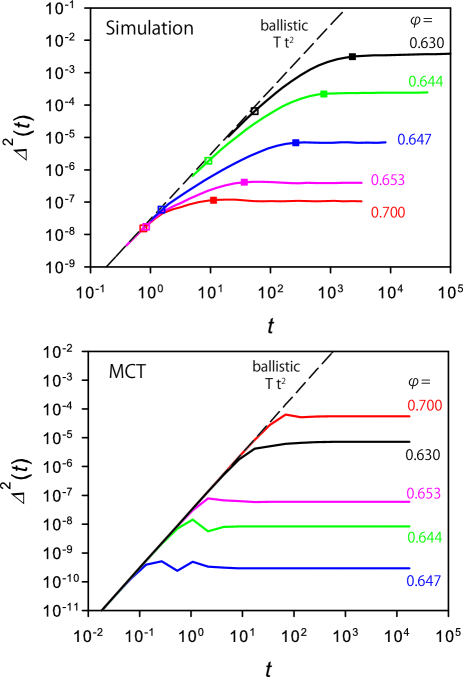
Figure 1: Top: Time dependence of the mean-squared displacements (MSD) obtained from simulation of harmonic spheres at constant temperature, $T=10^{-8}$, for volume fractions ranging from above to below the jamming density $\varphi_{J}\approx 0.647$. Open squares indicate the microscopic time scale $\tau_{0}$ where dynamics deviates from ballistic behavior. Filled squares indicate the time scale $t^{\star}$, which marks convergence of the MSD to its long-time plateau value. Both time scales decrease with $\varphi$, but their ratio is maximum near $\varphi_{J}$. Bottom: Time dependence of the MSD predicted by the MCT at the same state points. There is no decoupling between $\tau_{0}$ and $t^{\star}$ near $\varphi_{J}$, and the plateau value has a non-monotonic density dependence.

A closer look at the time dependence of the MSD reveals a very interesting behavior in the vicinity of the jamming transition. To this end, it is useful to introduce the microscopic time scale, $\tau_{0}$, which coincides with the moment where the MSD starts to deviate from its short-time ballistic behavior. This timescale $\tau_{0}$ is indicated by open squares in Fig. 1. Physically, it means that particles do not feel their environment for $t<\tau_{0}$. A second relevant timescale, $t^{\star}$, characterizes the time dependence of the MSD. It corresponds roughly to the timescale at which the MSD reaches its plateau value. This corresponds to the time it takes to the particles to fully explore their ‘cage’. This second timescale is indicated by the filled squares in Fig. 1. The precise definitions of these timescales can be found in our previous work criticality .

Clearly, while both $\tau_{0}$ and $t^{\star}$ decrease when the system is compressed, their ratio evolves in a striking non-monotonic manner with density, with a maximum occurring very close to $\varphi\approx\varphi_{J}$. This observation means that, when measured in units of the microscopic time scale $\tau_{0}$, vibrations occur over a timescale $t^{\star}$ that is very large near $\varphi_{J}$, but decreases as the packing fraction moves away from $\varphi_{J}$ on both sides of the jamming transition. This is closely related to the emergence of dynamic criticality criticality or soft modes reviewmodes as the jamming transition is approched, $|\varphi-\varphi_{J}|\to 0$ and $T\to 0$, with clear signatures in the vibrational dynamics at finite temperatures.

We now compare these results to the MCT predictions deduced after feeding the MCT equations with the ‘exact’ static structure factor $S(k)$ measured in the computer simulations at the state points represented in Fig. 1. First, we find that the solution of the MCT equations corresponds to glassy states, for which the long time limit of all correlation functions is finite. The bottom panel of Fig. 1 shows the MCT results for the MSD $\Delta^{2}(t)$ at the same state points as in the top panel. These results show similarities and differences with the simulation results.

The basic time dependence of $\Delta^{2}(t)$ is similar to the simulation results. The MSD show an initial ballistic regime at very short time, and they all reach a plateau at long time. A first difference with the simulations is that the density dependence of this plateau height decreases with compression in the hard sphere regime, but increases with density above the jamming density, which is at odds with the numerical results. Regarding the details of the time dependence, the MCT solution predicts that the time scales $\tau_{0}$ and $t^{\star}$ evolve together with a ratio $t^{\star}/\tau_{0}$ that is roughly independent of density. There is therefore no separation between microscopic and long time scales in these results, and the dynamic criticality of the jamming transition is not reproduced by the theory.

This failure is perhaps not too surprising as the initial theory was not devised to treat the jamming problem. However, we notice that soft modes are directly related to clear signatures in the pair correlation function $g(r)$ at short separation $r\approx a$, which we introduced in the dynamic equations to produce the results in Fig. 1. These results indicate, however, that this is not enough to reproduce the dynamics observed numerically.

III.2 Evolution of the Debye-Waller factor

From the time depencence of the MSD, we can extract the long-time limit,

$$\Delta^{2}(\infty)=\lim_{t\to\infty}\Delta^{2}(t),$$ (15)

which is called the Debye-Waller (DW) factor. We perform a quantitative analysis of its evolution over a wide range of temperatures and densities.

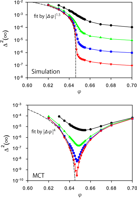
Figure 2: Volume fraction dependence of the long-time limit of the MSD from simulation (top) and from the MCT solution (bottom). Different curves correspond to different temperatures from $T=10^{-5}$ to $10^{-8}$ (from top to bottom). In simulations, the DW factor decreases with $\varphi$, with a singular drop near $\varphi_{J}$. By contrats, the predicted DW factor is non-monotonic with a sharp cusp near $\varphi_{J}$. The dashed lines indicate power laws for the hard sphere regime, $\varphi<\varphi_{J}$.

We show in Fig. 2 the density dependence of the DW factors at various temperatures, from $T=10^{-8}$ up to $T=10^{-5}$. In this density regime, the computer glass transition occurs near $T\approx 5\cdot 10^{-4}$. A first qualitative observation is the confirmation that for all temperatures, the DW factor decreases upon compression, indicating that particles have less space to perform vibrations at large density.

Second, this figure makes very clear the distinction between the two types of solids obtained on both sides of the jamming density. For $\varphi<\varphi_{J}$, which we called ‘hard sphere glass’, the DW factor becomes independent of the temperature at low $T$ and is uniquely controlled by $\varphi$. In this regime, particles are separated by a finite gap at very low temperatures, and they can explore this free volume regardless of the temperature value. On the other hand, when $\varphi>\varphi_{J}$, the DW factor is proportional to the temperature at low $T$. This corresponds to the situation where particles are vibrating in an energy minimum created by their neighbors. This temperature dependence simply corresponds to the low-temperature harmonic limit where equipartition of the energy yields $\Delta^{2}(\infty)\propto k_{B}T$. This is the regime we called ‘soft glass’.

The final observation is that upon lowering the temperature, the density dependence of the DW factor becomes singular on both sides of the transition, reflecting the emergence of the jamming singularity in the $T\to 0$ limit. Approaching the jamming transition from the hard sphere side, the DW factor shows a sharp drop, which is well-described by $\Delta^{2}(\infty)\sim(\varphi_{J}-\varphi)^{1.5}$. On the other hand, approaching jamming from the soft glass side, the DW factor diverges as $\Delta^{2}(\infty)\sim(\varphi-\varphi_{J})^{-0.5}$.

These two critical divergences are in fact directly related to the slowing down of the vibration discussed above criticality ; brito ; leche . To see this, it is useful to define a microscopic length scale $\ell_{0}$ associated to the microscopic time scale $\tau_{0}$ discussed above, through $\ell_{0}=\sqrt{T}\tau_{0}$. Notably, this length scale is vanishing as jamming is approached from the hard sphere side, $\ell_{0}\propto(\varphi_{J}-\varphi)$, simply reflecting the vanishing of the interparticle gap. On the soft sphere side, $\ell_{0}$ is not singular. Note that the amplitude of the vibrations quantified by the DW factor vanishes less rapidly than $\ell_{0}^{2}$ as $\varphi\to\varphi_{J}$, reflecting the emergence of ‘soft modes’, i.e. collective vibrational motion that allow large amplitude vibrations, $\Delta^{2}(\infty)\gg\ell_{0}^{2}$. By renormalizing the DW factor by the microscopic length scale, we obtain the density dependence of the adimensional amplitude of the vibrational motion, with

$$\frac{\Delta^{2}(\infty)}{\ell_{0}^{2}}\propto|\varphi_{J}-\varphi|^{-0.5},$$ (16)

for both hard sphere and soft glass regimes. This analysis shows that the amplitude of (adimensional) vibrations diverges as $T\to 0$ and $|\varphi-\varphi_{J}|\to 0$.

In Fig. 2 we present the MCT predictions for the DW factor for the same state points as in simulation. In the hard sphere regime, $\Delta^{2}(\infty)$ becomes independent of temperature as $T\to 0$, in agreement with the simulations. However, the DW factor also becomes independent of $T$ in the soft glass regime, in contradiction to the numerical findings. It means that MCT cannot account for the fact that dynamics in the soft glass is controlled by the amplitude of interparticle interactions rather than by entropic effects. This finding has consequences for the rheology of soft glasses, as discussed below.

Regarding the density dependence, MCT correctly predicts that the DW factor vanishes as $\varphi\to\varphi_{J}$ on the hard sphere side. Therefore, MCT is able to capture some of the singular features of the jamming transition. Mathematically, this is because the structure factor used as an input to the MCT dynamical equations becomes itself singular in this limit, which is responsible for the vanishing of the DW factor. We shall explore this limit in more detail below, but the numerical solution of the MCT equations in Fig. 2 shows that the resulting DW factor vanishes as $\Delta^{2}(\infty)\sim(\varphi_{J}-\varphi)^{4}$, i.e. with a power law that goes to zero much faster than the numerical observations. Intriguingly, the exponent 4 in this expression is even larger than the naive estimate $\Delta^{2}(\infty)\sim\ell_{0}^{2}\sim(\varphi_{J}-\varphi)^{2}$. This implies that MCT predicts that particles are localized over a lengthscale which is much smaller than the interparticle gap, which is not very physical. The second unphysical finding is the overall density dependence which is roughly symmetric on both sides of the jamming density, with the development of a sharp cusp near $\varphi_{J}$ as $T\to 0$ resulting from an incorrect treatment of the soft glass dynamics.

III.3 MCT predictions near the jamming transition

We now clarify analytically the nature of the MCT predictions near jamming, namely that $\Delta^{2}(\infty)$ vanishes on both sides of $\varphi_{J}$ with the same exponent. We first analyze the characteristic features of the static structure factor, and we then discuss the structure of the MCT equations near jamming.

III.3.1 Static structure factor near jamming

Since the sole input of the MCT equation is the static structure factor $S(k)$, the predicted singularity of the DW factor must come from changes in the structure. The pair structure of hard sphere packing near jamming has several relevant features gr1 ; gr2 ; gr3 . We find that the MCT equations are most sensitive to the simplest of these features, which correspond, in real space, to the appearance of a diverging peak at $r=a$ in the pair correlation function. Physically, this peak corresponds to the fact that at $\varphi=\varphi_{J}$ and $T=0$, particles have exactly $z=2d$ contacts, i.e. neighbors located at the distance $r=a$. Close to jamming, $|\varphi-\varphi_{J}|\ll\varphi_{J}$, this peak has a finite height,

$$g_{max}\sim\frac{1}{|\varphi-\varphi_{J}|},$$ (17)

and a finite width $|\varphi-\varphi_{J}|$, such that the peak turns into a delta function in the limit $\varphi\to\varphi_{J}$.

At first glance, the structure factor $S(k)$ near jamming appears not very different from normal fluids gr2 . It consists of a first diffraction peak near $k=2\pi/a$, followed by subsequent peaks at larger wavevectors. However, the diverging contact peak implies that the peaks at large $k$ have an amplitude which decreases more slowly than in simple liquids. We find that near the jamming density the envelope of the peaks of $S(k)-1$ first decreases as $k^{-1}$, followed by a crossover to a $k^{-2}$ behavior. When $\varphi$ gets closer to $\varphi_{J}$, the crossover wavevector $k^{\star}$ between these two power laws occurs at larger $k$, and it scales as $k^{\star}\sim g_{max}$. In summary, we find the following behaviour:

$$\mbox{peak heights of}\ [S(k)-1] \approx \frac{1}{k},\ \ \ \ \ 1\ll k\ll g_{max},$$ (18)

$$\approx \frac{g_{max}}{k^{2}},\ \ \ g_{max}\ll k.$$

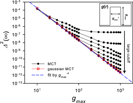
Figure 3: Evolution of the Debye-Waller factor approaching the jamming transition from the hard sphere side, parametrized the maximum $g_{max}\sim 1/|\varphi_{J}-\varphi|$ of the first peak of the pair correlation function. The DW factor predicted by the full MCT equation Eq. (9) (filled symbols) converges for a large enough cutoff to the result obtained from the Gaussian approximated MCT equation Eq. (21) (open symbols) using the simplified pair correlation function shown in the inset. All solutions agree with $\Delta^{2}(\infty)\approx g_{max}^{-4}$, and with the full MCT solution in Fig. 2.

To make analytic progress, we introduce a simplified model for the pair correlation $g(r)$ near jamming,

$$g(r)=g_{max},\quad{\rm for}\,\,1\leq r\leq 1+g_{max}^{-1},$$ (19)

and $g(r)=0$ otherwise. This model $g(r)$ is illustrated in the inset of Fig. 3. The Fourier transform of this rectangular function can be easily performed, and provides the scaling behavior of $S(k)$,

$$S(k)-1 \approx \frac{\sin(k)}{k},\ \ \ \ \ 1\ll k\ll g_{max},$$ (20)

$$\approx \frac{g_{max}\cos(k)}{k^{2}},\ \ \ \ \ g_{max}\ll k,$$

which is essentially the same as Eq. (18). In the limit of the jamming density, $S(k)$ becomes $S(k)-1\sim\sin(k)/k$, which is exactly the Fourier transform of the delta function in three dimensions. This means that the model Eq. (19) captures the large $k$ behavior of the real $S(k)$ correctly.

We have solved the MCT equations with the Fourier transform of Eq. (19) as an input for the structure factor. In Fig. 3 we show the evolution of the DW factor parameterized by the value of $g_{max}$, which diverges as $\varphi\to\varphi_{J}$. We present the results of the numerical solution obtained for different values for the wavevector cutoff, $N_{k}\Delta k$, showing that when the numerical solution has converged, a perfect agreement is obtained for the evolution of the DW factor from the numerically determined structure factor, and from the simplified model Eq. (19). Both MCT solutions, when properly converged, result in the scaling behavior $\Delta^{2}(\infty)\approx g_{max}^{-4}\sim(\varphi_{J}-\varphi)^{4}$. This agreement shows that the MCT solution is dominated by the large $k$ behavior of the $S(k)$, Eq. (18), and therefore is well captured by our simplified model in Eq. (19).

III.3.2 Analysis of the MCT equation: Gaussian approximation

To finally analyze the origin of the power law $\Delta^{2}(\infty)\approx g_{max}^{-4}$, we introduce a simplified version of the MCT equation, called Gaussian approximated MCT. Assuming that $F(k,t)$ and $F_{s}(k,t)$ have a Gaussian wavevector dependence and that $F(k,t)\approx S(k)F_{s}(k,t)$, which is the so-called Vineyard approximation (both conditions accurately hold in the full MCT solution), the MCT equation can be analytically simplified ikedamct . The long-time limit of this simplified MCT equations becomes

$$\begin{aligned} \frac{1}{\Delta^{2}(\infty)}=\frac{\rho}{6\pi^{2}}\int dk\ k^{4}c(k)^{2}e^{-2\Delta^{2}(\infty)k^{2}}.\end{aligned}$$ (21)

This equation takes $S(k)$ as a sole input (the direct correlation $c(k)$ follows directly from $S(k)$) as in the case of the full MCT equations. We again solve this equation numerically, and show the results in Fig. 3 as open squares. The solution perfectly agrees with the solution of the full MCT equation with the full $S(k)$.

The advantage of the formulation in Eq. (21) is that the asymptotic behaviour of the DW factor can now be understood analytically. Using the behaviour of $S(k)$ in Eq. (20), the integrant in Eq. (21) becomes $k^{2}e^{-2\Delta^{2}(\infty)k^{2}}$ for $k\ll g_{max}$, and $g_{max}^{2}e^{-2\Delta^{2}(\infty)k^{2}}$ when $k\gg g_{max}$. Here we omitted the square of trigonometric functions since they only give constant contributions. When $\Delta^{2}(\infty)\ll g_{max}^{-2}$, the integral is dominated by the contribution from $k\gg g_{max}$. This integral can be performed as a Gaussian integral, and this gives $\Delta^{2}(\infty)\approx g_{max}^{-4}$, which also agrees with the assumption $\Delta^{2}(\infty)\ll g_{max}^{-2}$, and with the observation from the full MCT equation.

In summary, by simplifying the full MCT treatment with the exact $S(k)$ using both a simplified model for $g(r)$ and a Gaussian approximation of the MCT equations, we can establish analytically the MCT result $\Delta^{2}(\infty)\sim(\varphi_{J}-\varphi)^{4}$, which is mainly controlled by the large $k$ behaviour of $S(k)$, produced by the divergence of the contact peak in $g(r)$.

III.4 Discussion of the MCT near jamming

We have unveiled two distinct features of the MCT predictions for the DW of harmonic spheres near the jamming transition.

First, we discussed the behaviour in the hard sphere regime, where a power law vanishing of the DW factor with a large exponent is found. We revealed that this power law is dominated by the behavior of the static structure factor at large wavevector $k^{\star}\gg g_{max}$. Since $1/k^{\star}$ represents the typical gap between particles, this finding implies that the MCT equations are actually controlled by lengthscales which are smaller than the typical gap. This is in clear disagreement with the numerical finding that the DW factor corresponds to an amplitude for the vibrations that is actually much larger the interparticle gap.

The second problem is more general, and thus more severe. In the soft glass regime, $\varphi>\varphi_{J}$, the predicted DW factor not only has the incorrect asymptotic behaviour, but it also has incorrect temperature and density dependences. This results from the fact that the solution of the MCT is controlled by $g_{max}$, while in the soft glass regime the system simply vibrates harmonically near the energy minimum. This physics is not captured by the MCT equations which instead again describe this harmonic solid as an ‘entropic’ system. This results in the prediction of a DW factor that remains finite as $T\to 0$ at large density, instead of the linear temperature dependence expected in this limit. We note that this problem is not specific to harmonic spheres and is actually very general for systems with continuous pair potentials, as will be shown in Sec. V where Lennard-Jones particles are considered.

IV Hard spheres and soft glasses under flow

In this section, we study the shear rheology of hard sphere and soft glasses extending the results in Sec. III to include shear flow. We start with the analysis on the flow curves and then provide a more detailed discussion of the yield stress behavior.

IV.1 Flow curves

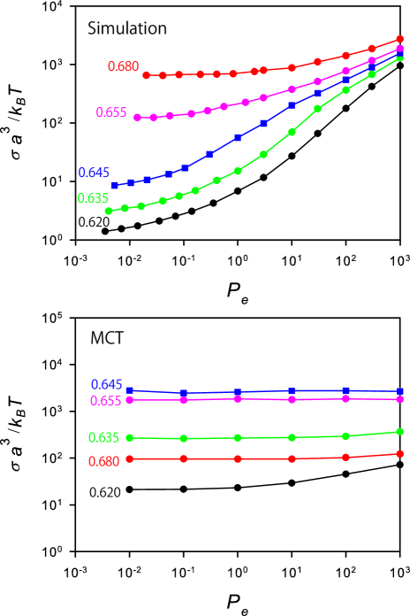
Figure 4: Top: Flow curves obtained from simulation of harmonic spheres at $T=10^{-6}$ and various volume fractions. A finite yield stress exists for all $\varphi$, which increases monotonically with the density. The athermal rheology of soft repulsive particles near jamming appears at large Peclet number, $P_{\rm e}>1$. Bottom: The MCT flow curves for the same state points as the top panel produce a finite yield stress at all $\varphi$ which is maximum near $\varphi_{J}\approx 0.647$, but decreases with $\varphi$ above jamming.

We start with a brief review of the simulation results for the flow curves of harmonic spheres ikeda . In the top panel of Fig. 4, we present several flow curves, $\sigma=\sigma(\dot{\gamma})$, at low temperature $k_{B}T/\epsilon=10^{-6}$ and various densities crossing the jamming density $\varphi_{J}$. We use adimensional units for both the stress scale (using $k_{B}T/a^{3}$ as thermal stress unit), and for the shear rate (using the Peclet number $P_{\rm e}=\dot{\gamma}a^{2}\xi/(k_{B}T)$).

First, we focus on the slow shear rate regime, $P_{\rm e}<1$. All the flow curves show that the stress approaches a constant value, the yield stress $\sigma_{Y}=\lim_{\dot{\gamma}\to 0}\sigma(\dot{\gamma})$. The yield stress increases rapidly with increasing the density. At lower density in hard sphere regime $\varphi<\varphi_{J}$, the stress is $\sigma_{Y}a^{3}/k_{B}T=\mathcal{O}(1)$, indicating the entropic nature of the stress, and it increases rapidly when the jamming transition is crossed, suggesting that it is not controlled by entropic forces alone in this regime.

Next, we focus on the fast shear rate regime, $P_{\rm e}>1$. In this regime, the flow curve shows complex and interesting behavior ikeda . At low density, the flow curve exhibits a crossover between strong shear-thinning when $P_{\rm e}<1$ to Newtonian behavior when $P_{\rm e}>1$. This shows that a system that looks solid at low $P_{\rm e}$ in fact appears as a fluid when $P_{\rm e}$ becomes large, characterized by an ‘athermal’ Newtonian viscosity. This viscosity increases rapidly with the density, and this Newtonian regime disappears above the jamming density, where it is replaced by the emergence of a finite yield stress.

We solved the MCT equation, Eq. (11), at the desired shear rate and with the static structure factor obtained from simulation at the desired density and temperature, following the same procedure as for the mean-squared displacement in the previous section. The bottom panel of Fig. 4 shows the flow curves obtained within MCT. As for the numerical results, the MCT flow curves at these state points are all approaching a finite yield stress at low shear rate, implying that MCT correctly predicts that these glass states offer a finite resistance to shear flow.

In the hard sphere regime, the yield stress increases rapidly with density, which qualitatively agrees with the numerical observations. However, the yield stress is found to decrease with density in the soft glass regime, in disagreement with the simulation results. This incorrect behavior is very similar to the one reported for the vibrational dynamics in the previous section, and we will argue below that it has the same origin.

Finally, we focus on the MCT predictions for $P_{\rm e}>1$. The MCT flow curves in this regime do not exhibit the interesting behavior observed in the numerical simulations. This is not very surprising as the MCT under shear flow is specifically designed to treat systems controlled by thermal fluctuations, which become inefficient when $P_{e}>1$. This result nevertheless clearly reveals that a naive extension of the MCT will not be sufficient to treat the interesting zero-temperature shear rheology of soft particle systems, which is currently the focus of a large interest ikeda ; softmatter ; olsson ; boyer ; lerner .

IV.2 Temperature and density evolution of the yield stress

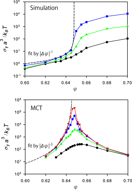
Figure 5: Top: Volume fraction dependence of the yield stress from the simulation from $T=10^{-5}$ to $10^{-7}$ (bottom to top). The yield stress increases monotonically with the emergence of sharp singularities near $\varphi_{J}$ as $T\to 0$. Bottom: MCT predictions for the same state points with $T=10^{-8}$ added. The yield stress is non-monotonic with a sharp cusp near $\varphi_{J}$. The dashed lines indicate power laws for the hard sphere regimes, $\varphi<\varphi_{J}$.

We finally arrive at the analysis of the yield stress in hard sphere and soft glasses.

We show in Fig. 5 the density dependence of the yield stress $\sigma_{Y}$ measured in the numerical simulation of harmonic spheres at various temperatures. These data confirm that the yield stress increases monotonically upon compression, as was observed in the flow curves. As in the case of the Debye-Waller factor, the temperature dependence of the yield stress is different on both sides of the jamming. For $\varphi<\varphi_{J}$, the entropic nature of the yield stress is obvious since it becomes proportional to temperature. In the adimensional represention of Fig. 5, this means that $\sigma a^{3}/(k_{B}T)$ becomes uniquely controlled by $\varphi$ in the hard sphere regime.

On the other hand, when $\varphi>\varphi_{J}$, the nature of the yield stress changes from being entropic to being controlled by the energy scale governing the particle repulsion, i.e. $\sigma_{Y}\sim\epsilon/a^{3}$. In the adimensional representation of Fig. 5, the data become proportional to $\epsilon/(k_{B}T)$. In this regime, the stress does not originate from thermal collisions between hard particles, but stems from direct interactions between particles interacting with a soft potential characterized by the energy scale $\epsilon$.

Having clarified the temperature dependence in the two regimes, we turn to the density dependence which becomes singular around the jamming density when temperature becomes small, mirrorring again the behavior of the DW factor. In the hard sphere regime, the yield stress increases rapidly as $\varphi_{J}$ approaches, with

$$\sigma_{Y}\sim\frac{k_{B}T}{a^{3}}\frac{1}{(\varphi_{J}-\varphi)}.$$ (22)

In the soft glass regime at low $T$, the yield stress vanishes when the jamming transition is approached, with

$$\sigma_{Y}\sim\frac{\epsilon}{a^{3}}(\varphi-\varphi_{J}).$$ (23)

These two asymptotic behaviors are clearly observed in Fig. 5.

The bottom panel of Fig. 5 presents the MCT predictions for the yield stress for the same state points. The theory predicts that the yield stress results from entropic forces on both sides of the transition, failing to recognize the change to the soft glass regime dominated by interparticle forces. As a result, the theory incorrectly predicts the emergence of a cusp as $T\to 0$, with a symmetric divergence of the yield stress on both sides of $\varphi_{J}$, which is only observed on the hard sphere side in the simulations. At the quantitative level, the MCT predicts a power law divergence on the hard sphere side, $\sigma_{Y}\sim\frac{k_{B}T}{a^{3}}(\varphi_{J}-\varphi)^{-3}$, but the exponent 3 differs from the numerical result although the (entropic) prefactor has the right scaling.

Overall, the degree of consistency between theory and simulation for the yield stress is very similar to the one deduced from the analysis of the DW factor in the previous section. In the following section, we rationalize this similarity.

IV.3 MCT predictions near the jamming transition

We now provide an explanation for the MCT prediction of the yield stress divergence $\sigma_{Y}\propto(\varphi_{J}-\varphi)^{-3}$ in the hard sphere regime, and of the qualitatively incorrect scaling found in the soft glass regime. To do so, we analyze the structure of the MCT equations under shear flow.

In the MCT framework, the stress is expressed as an integral over time and wavevector, see Eq. (14). For the present analysis, it is useful to rewrite the integral as

$$\sigma=\dot{\gamma}\int^{\infty}_{0}dt\ G(t),$$ (24)

where

$$G(t)=\frac{k_{B}T\rho^{2}}{60\pi^{2}}\int^{\infty}_{0}\!\!dk\ \frac{k^{5}c^{\prime}(k)c^{\prime}(k(t))}{k(t)}F_{t}(k(t),t)^{2},$$ (25)

is the MCT expression of the transient stress auto-correlation function. Using this expression, we can analyze the shear stress in terms of the relaxation behavior of $G(t)$.

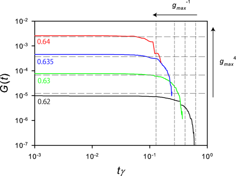
Figure 6: Time dependence of the stress autocorrelation function $G(t)$ obtained from the numerical solution of the MCT equations under shear flow in the hard sphere regime approaching jamming, for $T=10^{-6}$ for $P_{\rm e}=10^{-3}$. The horizontal and perpendicular dashed lines respectively scale as $g_{max}^{4}$ and $g_{max}^{-1}$, in agreement with Eqs. (27, 28).

In Fig. 6, we show $G(t)$ for $T=10^{-6}$ and several densities in the hard sphere regime below jamming. The shear rate is fixed at $P_{\rm e}=10^{-3}$, where the stress is nearly equal to the yield stress. As discussed in the previous section, the yield stress increases rapidly with approaching jamming. The data in Fig. 6 show that the stress increase results from the combination of two different contributions. A first factor is the sharp increase of the plateau height of $G(t)$ with density. The second factor is the decrease of the relaxation time of $G(t)$ with increasing the density. We now analyse these two factors separately.

When $t$ is small as $t\dot{\gamma}\ll 1$, the advected wavevector $k(t)$ is essentially equal to the wavevector at rest, $k(t_{micro}\ll t\ll\dot{\gamma}^{-1})\approx k$, where $t_{micro}$ is the microscopic time to reach the plateau. In this case, the sheared MCT equations Eq. (11) is nothing but the usual MCT equation, Eq. (5). Thus, the transient intermediate scattering function $F_{t}(k,t)$ in this regime can be accurately approximated by the usual intermediate scattering function $F(k,t)$, with no influence from the wavevector advection. In this regime, the plateau height of $G(t)$ can be rewritten as

$$\begin{aligned} G_{p}\approx\frac{k_{B}T\rho^{2}}{60\pi^{2}}\int^{\infty}_{0}\!\!dk\ k^{4}c^{\prime}(k)^{2}F(k,t)^{2}.\end{aligned}$$ (26)

This expression is exactly the one provided by MCT for the shear modulus of the glass at rest nagele . Furthermore, the behavior of $c^{\prime}(k)$ at large $k$ is the same as $c(k)$, since $c(k)$ is asymptotically a product of a fast oscillating function and a slowly decreasing function of $k$ as in Eq. (20), and thus the amplitude of $c(k)$ and $c^{\prime}(k)$ is asymptotically the same. Therefore, Eq. (26) is also essentially equivalent to the right hand side of Eq. (21), which enters the expression of the DW factor. This means the plateau height behaves as

$$G_{p}\sim k_{B}Tg_{max}^{4},$$ (27)

showing that the shear modulus scales with density as the inverse of the DW factor, with a temperature prefactor revealing its entropic nature. In Fig. 6, we represented dashed lines at levels scaling with $g_{max}^{4}$, which confirm that $G_{p}$ indeed follows Eq. (27).

The second factor contributing to the scaling of the shear stress is the relaxation time of $G(t)$. In the sheared MCT, the memory function becomes explicitly time dependent because of the advection of the wave vectors. A decoupling between $k$ and the advected $k(t)$ occurs at long time, which results in a dephasing of the oscillations of $c(k)$ and $c(k(t))$. We have shown in the previous section that the MCT integral are dominated by a Gaussian contribution $\sim\exp(-2\Delta^{2}(\infty)k^{2})$, showing that we need to consider the decoupling of wave vectors for $k\sim 1/\Delta(\infty)$. This occurs after a time $t_{Y}$ such that $k(t_{Y})-k=\mathcal{O}(1)$. This produces an estimate for the relaxation time of the stress autocorrelation function,

$$t_{Y}\dot{\gamma}\sim k^{-1/2}\sim g_{max}^{-1}.$$ (28)

We plot this estimate in Fig. 6 with vertical lines scaling with $g_{max}^{-1}$. Clearly, these lines agree very well with the relaxation time of $G(t)$ obtained from the numerical resolution of the MCT equations. Since we focus on the relaxation dynamics of the system subjected to the shear flow starting at time $t=0$, $t_{Y}$ measures the time it takes the glass to yield. We can therefore identify $\gamma_{Y}=t_{Y}\dot{\gamma}$ with the yield strain.

By combining the MCT prediction for the divergence of the shear modulus near jamming as $G_{p}\approx k_{B}T(\varphi_{J}-\varphi)^{-4}$, and for the vanishing of the yield strain as $\gamma_{Y}\approx(\varphi_{J}-\varphi)^{1}$, we obtain the divergence of the yield stress as $\sigma_{Y}\approx G_{p}\gamma_{Y}\approx k_{B}T(\varphi_{J}-\varphi)^{-3}$. This scaling law agrees very well with the numerical solution of the MCT equations shown in Fig. 5, as announced.

IV.4 Discussion of the MCT under flow near jamming

The above analysis clarifies that the MCT under shear flow makes predictions for the yield stress which are direct consequences of the behavior obtained from the MCT dealing with the glass dynamics at rest. Within MCT, the yield stress can be expressed as the product of the shear modulus and the yield strain, $\sigma_{Y}=G_{p}\gamma_{Y}$, and the shear modulus in the MCT framework, Eq. (26), is closely related to the DW factor. Thus, the discussions of the MCT predictions near jamming for the DW factor and the yield stress are essentially the same. In the hard sphere regime, MCT correctly describes the entropic nature of the yield stress and its divergence as $\varphi_{J}$ is approached, but the critical exponent for the divergence is too strong. In the soft glass regime, the theory incorrectly predicts a scaling of the yield stress with $k_{B}T$, failing to detect the direct influence of the particle interactions.

However, we wish to note that MCT provides a new prediction for the yield strain $\gamma_{Y}$ in the hard sphere regime, $\gamma_{Y}\approx(\varphi_{J}-\varphi)$. This is an interesting novel critical behaviour, although the predicted value for the associated critical exponent is not correct. Indeed, in the simulations one has $\sigma_{Y}\sim(\varphi_{J}-\varphi)^{-1}$ ikeda , while the shear modulus scales with a different exponent, $G_{p}\sim(\varphi_{J}-\varphi)^{-1.5}$ britoepl . This indicates that the yield strain actually vanishes as $\gamma_{Y}\approx(\varphi_{J}-\varphi)^{0.5}$. Note that recent experiments in dense emulsions show that the yield strain decreases when the jamming transition is approached mason .

A simple argument can rationalize the critical scaling of the yield strain. The yielding predicted by the MCT occurs due to the decoupling between the wavevector and the advected one at the ‘relevant’ length scale. Using the correct value of the interparticle gap for this length scale, one directly predicts that yielding occurs when the typical gap between neighboring particles $\delta\sim|\varphi-\varphi_{J}|$ is blurred by the shear deformation. (A similar argument was used in Ref. criticality to discuss thermal effects.) The shear flow causes a transverse displacement of particles over a length $\gamma a$, and this causes a change in the interparticle distance $\gamma^{2}a$. Yielding then occurs when $\gamma_{Y}^{2}a\approx\delta$, which gives $\gamma_{Y}\approx(\varphi_{J}-\varphi)^{0.5}$, as observed numerically. Note that the argument can be repeated above the jamming transition in the soft glass regime. Also in this regime, there is a mismatch between the scalings of yield stress olsson ; ikeda and shear modulus ohern1 , indicating that the yield strain vanishes as $\gamma_{Y}\approx(\varphi-\varphi_{J})^{0.5}$. This is again consistent with the idea that the particle overlap $\delta\sim|\varphi-\varphi_{J}|$ is the relevant length scale.

V Lennard-Jones glass dynamics

In this section, we focus on Lennard-Jones particles, with two main justifications. First, this allows us to treat a very different type of material, as Lennard-Jones fluids are often taken as simple models to study metallic glasses binder . A second goal is to investigate further the generality of the findings of the previous sections concerning the difficulty encountered by MCT in describing amorphous materials when solidity emerges from direct, continuous interparticle forces. We first analyze the structure of the Lennard-Jones glass, then its vibrational dynamics, and we finally study the yield stress measured under shear flow.

V.1 Glass structure factor

To solve the MCT equations under shear flow, we need the glass structure factor as an input. We use the structure factor measured in low-temperature numerical simulations of the monodisperse Lennard-Jones system. However, since we use a monodisperse system, crystallization takes place if we use a temperature which becomes too close to the glass transition and diffusive motion becomes possible. To avoid this problem, we need to restrain ourselves on relatively low temperatures.

To extend our analysis to higher temperatures, we implement a second strategy. We use statistical mechanics to predict the structure factor of the Lennard-Jones fluid and glass states combining the hyper-netted chain approximation for the fluid hansen , to the replica approach of Ref. mp for the glass. While we do not expect this approach to be very accurate, it still provides structure factors that are qualitatively correct down to very low temperatures, encompassing both fluid and glass states. Using this approach, we find that MCT predicts a kinetic arrest occurring at $T_{mct}\approx 1.2$, while the replica approach yields a Kauzmann transition at lower temperature, near $T_{K}\approx 0.9$. Above $T_{K}$, $S(k)$ is identical to the prediction of the hypernetted chain approximation, while below $T_{K}$ the glass structure differs from the liquid state approximation mp .

The key point of both approaches is that when $T$ becomes smaller than the computer glass transition, $S(k)$ rapidly converges towards its $T\to 0$ limit, and has actually a very weak temperature dependence in the glass phase. By contrast with the jamming point, however, $S(k)$ does not develop any kind of singularity even as $T\to 0$. This directly implies that DW factor and yield stress should behave smoothly in the glass phase of the Lennard-Jones system.

The reason for this becomes clearer if one focuses on the pair correlation function. In the frozen glass state, the distance between any two particles fluctuates around its average value with a variance proportional to $k_{B}T$. However, since the structure is fully amorphous, the spatially averaged pair correlation function remains non-singular as $T\to 0$ because the successive correlation peaks are broadened by the quenched disorder imposed by the amorphous structure.

Therefore, when lowering $T$, there exists a temperature crossover, $T_{q}$, below which the thermal broadening of the peaks in the pair structure becomes smaller than the broadening due to the quenched disorder. When $T<T_{q}$, $S(k)$ and $g(r)$ do not depend on $T$ anymore, and the solution to the MCT dynamic equations remain the same as $T$ is decreased further. We shall see that MCT yields physically incorrect solutions below $T_{q}$.

V.2 Temperature evolution of the Debye-Waller factor

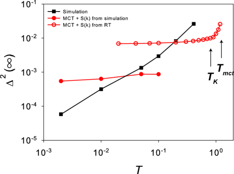
Figure 7: Temperature dependence of the DW factor obtained from direct numerical simulation (filled squares) and from MCT using either the numerically measured structure factor (filled circles) or a statistical mechanics approach (Replica Theory, open circles). While the simulation results indicate a linear dependence on $T$, the MCT solution suggests a singular $T$-dependence near $T_{mct}$ followed by a rapid saturation to an unphysical $T$-independent value.

We start our analysis of the MCT predictions for the Lennard-Jones glass with the characterization of the vibrational dynamics. We focus on the temperature dependence of the DW factor for a fixed number density, $\rho=1.2$.

The temperature dependence of the DW factor $\Delta^{2}(\infty)$ obtained from direct numerical simulations is plotted in Fig. 7 together with the results from the MCT solution. The simulation results (filled square) show that the DW factor is proportional to temperature when temperature becomes small, which is the same behavior as observed for the soft glass in Sec. III. This corresponds again to the limit of the Einstein harmonic solid where the amplitude of the vibrations around the average position is proportional to $k_{B}T$, as a direct result of equipartition of the energy. The data in Fig. 7 indicate that this linear behaviour is obeyed to a good approximation nearly up to the glass transition temperature.

The MCT analysis performed using the static structure factor obtained from simulation is shown with filled circles, which indicate that the DW factor is nearly independent of temperature in this regime. This result follows from the above discussion of the static structure which is also temperature independent, but clearly contradicts the numerical simulations. This discrepancy is in fact equivalent to the findings obtained in the soft glass regime of harmonic spheres.

Finally, using the analytic structure factor, we can follow the DW factor to higher temperatures and describe the emergence of a finite DW factor, $\Delta^{2}_{c}$, at the predicted mode-coupling transition, $T_{mct}=1.2$. The theory then predicts an abrupt temperature dependence characterizing by a square root singularity gotze , $\Delta^{2}(\infty)\sim\Delta^{2}_{c}-a\sqrt{T_{mct}-T}$, where $a$ is a numerical prefactor. However, the temperature evolution of the DW factor again rapidly saturates to a $T$-independent value.

V.3 Temperature evolution of the yield stress

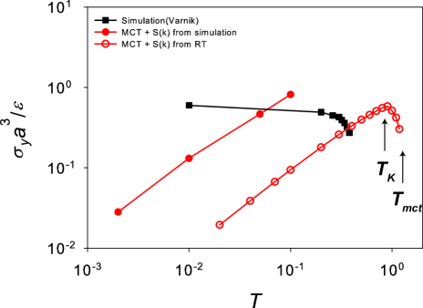
Figure 8: Temperature dependence of the yield stress obtained from direct numerical simulation (filled squares) and from MCT using either the numerically measured structure factor (filled circles) or a statistical mechanics approach (Replica Theory, open circles). While the simulation results indicate a nearly temperature independent yield stress, $\sigma_{Y}\sim\epsilon/a^{3}$, the MCT solution produces instead an ‘entropic’ yield stress vanishing linearly with $T$ at low $T$.

We now analyze the temperature dependence of the yield stress of the Lennard-Jones model.

In Fig. 8, the yield stress obtained from earlier simulations yieldLJ ; yieldLJ2 and from the MCT equations are plotted as a function of the temperature. From the discussion in Sec. IV for the soft glass, we expect the yield stress of the Lennard-Jones system to be controlled by the interaction energy between particles, and we choose therefore to plot the stress in adimensional units, $\sigma\to\sigma/(\epsilon/a^{3})$, where $\epsilon$ represents now the attractive depth of the Lennard-Jones potential. Using this representation, we find that the numerical results for the yield stress are in fact weakly dependent on the temperature, rapidly saturating to the $T\to 0$ limit, $\sigma_{Y}(T=0)/(\epsilon/a^{3})\sim{\cal O}(1)$, as expected.

Performing the MCT analysis using the low temperature structure factor, we find that the predicted yield stress decreases linearly with the temperature. This is because in this regime $S(k)$ is nearly constant, and the MCT equations produce an incorrect ‘entropic’ yield stress, i.e. $\sigma_{Y}\sim k_{B}T$. Finally, using the analytic structure factor, we again find a yield stress which vanishes linearly with $T$ at low $T$, with a singular emergence near the mode-coupling singularity, mirrorring the behaviour obtained for the DW factor in Fig. 7.

Again, the discrepancy between simulations and MCT predictions regarding the physical origin of the yield stress is the same as the one uncovered in the above study of the soft glass regime of harmonic spheres. This shows that this result was not an artefact of the peculiar harmonic sphere system, nor was it related to singularities encountered near the jamming transition in this system. For Lennard-Jones particles, there is no jamming singularity in the density regime studied in the present section, but similar results are found for this well-known glass-forming model system.

VI Discussion

We have shown that mode-coupling theory provides ‘first-principles’ predictions for the emergence of the yield stress in amorphous solids, together with detailed predictions for the temperature and density dependences of the yield stress in various glassy materials, from hard sphere glasses to soft and metallic glasses.

For hard sphere glasses, the theory correctly predicts the emergence of solid behaviour with entropic origin, with a yield stress and shear modulus proportional to $k_{B}T$. The theory also predicts a divergence of the yield stress as the random close packing density is approached, but the predicted critical exponent is too large. We have shown that this is because MCT also considerably overestimates the degree of localization of the particles in the glass at rest near the jamming transition.

The theory fares more poorly for both soft glasses and metallic glasses, as it again predicts a yield stress proportional to $k_{B}T$ while solidity is in fact the result of direct interparticle forces, and scales instead as $\epsilon/a^{3}$, where $\epsilon$ is the typical energy scale governing particle interactions.

This means that while the flow curves predicted by MCT for a given material across the glass transition may have functional forms that are in good agreement with the observations, it is not clear whether the non-linear flow curves produced in the glass phase are physically meaningful for particles that cannot be represented as effective hard spheres.

The fact that the mode-coupling theory provides limited insight into solid phases is perhaps not surprising, as the theory was initially developed as an extension of liquid state theories gotze . However, since the theory describes the transformation into the arrested glass phase, the MCT predictions for the glass dynamics at rest and for the glass dynamics under shear flow have been worked out in detail, and often discussed in connection with experimentally relevant questions, such the Boson peak in amorphous systems gotze2 , and the non-linear flow of glasses fuchs4 .

Our study suggests that one should perhaps not try to apply MCT ‘too deep’ into the glass, but it must be noted that the theory itself can be applied arbitrarily far into the glass phase with no internal criterion suggesting that the procedure becomes inconsistent, as long as reliable estimates of the static structure factor are available.

For Lennard-Jones particles and the soft glass regime of harmonic spheres, we have discussed such a criterion. We suggested the existence of a temperature scale $T_{q}$ below which MCT predictions certainly become unreliable. This temperature is such that, below $T_{q}$, the averaged static structure becomes dominated by the quenched disorder instead of thermal fluctuations criticality . This implies that MCT predictions for glassy phases should be more reliable in the regime $T_{q}<T<T_{g}$. We note, however, that MCT only makes crisp predictions near the mode-coupling ‘singularity’ $T_{mct}$ (such as square root dependence of the DW factor and yield stress) but these are not easy to test since the real system is actually in a fluid state at $T_{mct}>T_{g}$.

More generally, we believe our work emphasizes the need for more detailed theoretical analysis of the non-linear response of amorphous solids to external shear flow to produce better theoretical understanding of the yield stress in disordered materials. Recent progress in the statistical mechanics of the glassy state using replica calculations gr3 ; mp ; PZ ; hugo ; yoshino provide detailed predictions for the thermodynamics, micro-structure, and shear modulus of glassy phases, that are, contrary to the MCT result exposed in this work, at least consistent with a low-temperature harmonic description of amorphous solids. One can hope that an these calculations can be extended to treat also the yield stress.

- (1) H. A. Barnes, J. Non-Newtonian Fluid Mech. 81, 133 (1999).
- (2) P. Coussot, Rheometry of Pastes, Suspensions, and Granular Materials (Wiley, New York, 2005).
- (3) P. C. F. Moller, A. Fall and D. Bonn, Europhys. Lett. 87, 38004 (2009).
- (4) D. Bonn and M. M. Denn Science 324, 5933 (2009).
- (5) K. Binder and W. Kob, Glassy materials and disordered solids (World Scientific, Singapore, 2011).
- (6) L. Berthier and G. Biroli, Rev. Mod. Phys. 83, 587 (2011).
- (7) A. J. Liu, M. Wyart, W. van Saarloos and S. R. Nagel in Dynamical heterogeneities in glasses, colloids and granular materials, Eds.: L. Berthier, G. Biroli, J.-P. Bouchaud, L. Cipelletti, and W. van Saarloos, (Oxford University Press, Oxford, 2011).
- (8) M. van Hecke, J. Phys.: Condens. Matter, 22, 033101 (2010).
- (9) A. Ikeda, L. Berthier, and P. Sollich, Phys. Rev. Lett. 109, 018301 (2012).
- (10) A. Ikeda, L. Berthier, and P. Sollich, Soft Matter (at press), arXiv:1302.4271.
- (11) F. Scheffold, F. Cardinaux, and T. G. Mason arXiv:1305.5182.
- (12) G. Picard, A. Ajdari, F. Lequeux, and L. Bocquet, Phys. Rev. E 71, 010501 (2005).
- (13) J. C. Baret, D. Vandembroucq, and S. Roux, Phys. Rev. Lett. 89, 195506 (2002).
- (14) E. A. Jagla, Phys. Rev. E 76, 046119 (2007).
- (15) K. Martens, L. Bocquet, and J.-L. Barrat, Phys. Rev. Lett. 106, 156001 (2011).
- (16) L. Bocquet, A. Colin and A. Ajdari, Phys. Rev. Lett. 103, 036001 (2009).
- (17) P. Sollich, F. Lequeux, P. Hébraud, and M. E. Cates, Phys. Rev. Lett. 78, 2020 (1997)
- (18) P. Hébraud and F. Lequeux, Phys. Rev. Lett. 81, 2934 (1998).
- (19) L. Berthier, J.-L. Barrat and J. Kurchan, Phys. Rev. E 61, 5464 (2000).
- (20) W. Götze, Complex dynamics of glass-forming liquids: A mode-coupling theory (Oxford University Press, Oxford, 2008).
- (21) K. Miyazaki and D. R. Reichman, Phys. Rev. E 66, 050501 (2002).
- (22) K. Miyazaki, H. M. Wyss, D. A. Weitz and D. R. Reichman, Europhys. Lett. 75, 915 (2006).
- (23) M. Fuchs and M. E. Cates Phys. Rev. Lett. 89, 248304 (2002).
- (24) J. M. Brader, T. Voigtmann, M. E. Cates and M. Fuchs, Phys. Rev. Lett. 98, 058301 (2012).
- (25) M. Fuchs and M. E. Cates, J. Rheol. 53, 957 (2009).
- (26) M. Ballauff, J. M. Brader, S. U. Egelhaaf, M. Fuchs, J. Horbach, N. Koumakis, M. Krüger, M. Laurati, K. J. Mutch, G. Petekidis, M. Siebenbürger, T. Voigtmann and J. Zausch, Phys. Rev. Lett. 110, 215701 (2013).
- (27) M. Nauroth and W. Kob, Phys. Rev. E 55, 657 (1997).
- (28) L. Berthier and G. Tarjus Phys. Rev. E 82, 031502 (2010).
- (29) J. Mewis and N. J. Wagner, Colloidal suspension rheology (Cambridge University Press, Cambridge, 2012).
- (30) A. Ghosh, V. K. Chikkadi, P. Schall, J. Kurchan, and D. Bonn, Phys. Rev. Lett. 104, 248305 (2010).
- (31) K. Chen, W. G. Ellenbroek, Z. Zhang, D. T. N. Chen, P. J. Yunker, C. Brito, O. Dauchot, S. Henkes, W. van Saarloos, A. J. Liu, and A. G. Yodh, Phys. Rev. Lett. 105, 025501 (2010).
- (32) A. Ikeda, L. Berthier, and G. Biroli J. Chem. Phys. 138, 12A507 (2013).
- (33) L. Berthier and T. A. Witten, EPL 86, 10001 (2009); Phys. Rev. E 80, 021502 (2009).
- (34) C. S. O’Hern, S. A. Langer, A. J. Liu, and S. R. Nagel, Phys. Rev. Lett. 88, 075507 (2002).
- (35) L. Berthier, Phys. Rev. E 69, 020201(R) (2004).
- (36) L. Berthier and J.-L. Barrat, Phys. Rev. Lett. 89, 095702 (2002).
- (37) F. Varnik and O. Henrich, Phys. Rev. B 73, 174209 (2006).
- (38) J. P. Hansen and I. R. McDonald, Theory of Simple Liquids, (Elsevier, Amsterdam, 1986).
- (39) U. Bengtzelius, Phys. Rev. A 34, 5059 (1986)
- (40) L. Berthier, E. Flenner, H. Jacquin, and G. Szamel Phys. Rev. E 81, 031505 (2010).
- (41) C. Brito and M. Wyart, J. Chem. Phys. 131, 024504 (2009).
- (42) F. Lechenault, O. Dauchot, G. Biroli, and J.-P. Bouchaud, Europhys. Lett. 83, 46002 (2008).
- (43) A. Donev, S. Torquato and F. H. Stillinger, Phys. Rev. E 71, 011105 (2005).
- (44) L. E. Silbert, A. J. Liu and S. R. Nagel, Phys. Rev. E 73, 041304 (2006).
- (45) L. Berthier, H. Jacquin, and F. Zamponi Phys. Rev. E 84, 051103 (2011).
- (46) A. Ikeda and K. Miyazaki Phys. Rev. Lett. 104, 255704 (2010).
- (47) P. Olsson and S. Teitel, Phys. Rev. Lett. 99, 178001 (2007).
- (48) F. Boyer, E. Guazzelli, and O. Pouliquen, Phys. Rev. Lett. 107, 188301 (2011).
- (49) E. Lerner, G. Düring, and M. Wyart, Proc. Natl. Acad. Sci. USA 109, 4798 (2012).
- (50) G. Nägele and J. Bergenholtz J. Chem. Phys. 108, 9893 (1998).
- (51) C. Brito and M. Wyart, Europhys. Lett. 76, 149 (2006).
- (52) M. Mézard and G. Parisi J. Chem. Phys. 111, 1076 (1999).
- (53) W. Götze and M. R. Mayr, Phys. Rev. E 61, 587 (2000).
- (54) G. Parisi and F. Zamponi, Rev. Mod. Phys. 82, 789 (2010).
- (55) H. Jacquin, L. Berthier, and F. Zamponi, Phys. Rev. Lett. 106, 135702 (2011).
- (56) H. Yoshino, J. Chem. Phys. 136, 214108 (2012); S. Okamura and H. Yoshino, arXiv:1306.2777.