An improvement of the Feng-Rao bound for primary codes

Abstract

We present a new bound for the minimum distance of a general primary linear code. For affine variety codes defined from generalised $C_{ab}$ polynomials the new bound often improves dramatically on the Feng-Rao bound for primary codes [1, 10]. The method does not only work for the minimum distance but can be applied to any generalised Hamming weight.

Keywords: Affine variety code, $C_{ab}$ curve, Feng-Rao bound, footprint bound, generalised $C_{ab}$ polynomial, generalised Hamming weight, minimum distance, one-way well-behaving pair, order domain conditions.

MSC: 94B65, 94B27, 94B05.

1 Introduction

In this paper we present an improvement to the Feng-Rao bound for primary codes [1, 10, 9]. Our method does not only apply to the minimum distance but estimates any generalised Hamming weight. In the same way as the Feng-Rao bound for primary codes suggests an improved code construction our new bound does also. The new bound is particular suited for affine variety codes for which it often improves dramatically on the Feng-Rao bound. Interestingly, for such codes it can be viewed as a simple application of the footprint bound from Gröbner basis theory. We pay particular attention to the case of the affine variety being defined by a bivariate polynomial that, in the support, has two univariate monomials of the same weight and all other monomials of lower weight. Such polynomials can be viewed as a generalisation of the polynomials defining $C_{ab}$ curves and therefore we name them generalised $C_{ab}$ polynomials. We develop a method for constructing generalised $C_{ab}$ polynomials with many zeros by the use of $({\mathbb{F}}_{p^{m}},{\mathbb{F}}_{p})$-polynomials, that are polynomials returning values in ${\mathbb{F}}_{p}$ when evaluated in ${\mathbb{F}}_{p^{m}}$ (see, [21, Chap. 1]). Here, $p$ is any prime power and $m$ is an integer larger than $1$. With this method in hand we can design long affine variety codes for which our bound produces good results. The new bound of the present paper is closely related to an improvement of the Feng-Rao bound for dual codes that we presented recently in [8]. Recall from [9] that the usual Feng-Rao bound for primary and dual codes can be viewed as consequences of each other. This result holds when one uses the concept of well-behaving pairs or one-way well-behaving pairs. For weakly well-behaving pairs a possible connection is unknown. In a similar way as the proof from [9] breaks down for weakly well-behaving, it also breaks down when one tries to establish a connection between the new bound from the present paper and the new bound from [8]. We shall leave it as an open problem to decide if the two bounds are consequences of each other or not.

In the first part of the paper we concentrate solely on affine variety codes. For such codes the new method is intuitive. We start by formulating in Section 2 our new bound at the level of affine variety codes and explain how it gives rise to an improved code construction $\widetilde{E}_{imp}(\delta)$. Then we continue in Section 3 by showing how to construct generalised $C_{ab}$ polynomials with many zeros. In Section 4 we give a thorough treatment of codes defined from so-called optimal generalised $C_{ab}$ polynomials demonstrating the strength of our new method. In Section 5 we show how to improve the improved code construction $\widetilde{E}_{imp}(\delta)$ even further. This is done for the case of the affine variety being the Klein quartic. Having up till now only considered the minimum distance, in Section 6 we explain how to deal with generalised Hamming weights. Then we turn to the level of general primary linear codes lifting in Section 7 our method to a bound on any primary linear code. In Section 8 we recall the recent bound from [8] on dual codes, and in Section 9 we discuss the relation between this bound and the new bound of the present paper. Section 10 is the conclusion.

2 Improving the Feng-Rao bound for primary affine variety codes

Affine variety codes were introduced by Fitzgerald and Lax in [4] as follows. For $q$ a prime power consider an ideal $I\subseteq{\mathbb{F}}_{q}[X_{1},\ldots,X_{m}]$ and define

$$I_{q}=I+\langle X_{1}^{q}-X_{1},\ldots,X_{m}^{q}-X_{m}\rangle,$$ (1)

$$R_{q}={\mathbb{F}}_{q}[X_{1},\ldots,X_{m}]/I_{q}.$$

Let $\{P_{1},\ldots,P_{n}\}={\mathbb{V}}_{\mathbb{F}_{q}}(I_{q})$ be the corresponding variety over ${\mathbb{F}}_{q}$. Here, $P_{i}\neq P_{j}$ for $i\neq j$. Define the ${\mathbb{F}}_{q}$-linear map ${\mbox{ev}}:R_{q}\rightarrow{\mathbb{F}}_{q}^{n}$ by ${\mbox{ev}}(A+I_{q})=(A(P_{1}),\ldots,A(P_{n}))$. It is well-known that this map is a vector space isomorphism.

Definition 1.

Let $L$ be an ${\mathbb{F}}_{q}$ vector subspace of $R_{q}$. Define $C(I,L)={\mbox{ev}}(L)$ and $C^{\perp}(I,L)=\big{(}C(I,L)\big{)}^{\perp}$.

We shall call $C(I,L)$ a primary affine variety code and $C^{\perp}(I,L)$ a dual affine variety code. For the case of primary affine variety codes both the Feng-Rao bound and the bound of the present paper can be viewed as consequences of the footprint bound from Gröbner basis theory as we now explain.

Definition 2.

Let $J\subseteq k[X_{1},\ldots,X_{m}]$ be an ideal and let $\prec$ be a fixed monomial ordering. Here, $k$ is an arbitrary field. Denote by ${\mathcal{M}}(X_{1},\ldots,X_{m})$ the monomials in the variables $X_{1},\ldots,X_{m}$. The footprint of $J$ with respect to $\prec$ is the set

$$\Delta_{\prec}(J) = \{M\in{\mathcal{M}}(X_{1},\ldots,X_{m})\mid M{\mbox{ is not }}$$

$${\mbox{ \ \ \ \ \ the leading monomial of any polynomial in }}J\}.$$

Proposition 3.

Let the notation be as in Definition 2. The set $\{M+J\mid M\in\Delta_{\prec}(J)\}$ constitutes a basis for $k[X_{1},\ldots,X_{m}]/J$ as a vector space over $k$.

Proof.

See [2, Pro. 4, Sec. 5.3]. ∎

We shall make extensive use of the following incidence of the footprint bound (for a more general version, see [7]).

Corollary 4.

Let $F_{1},\ldots,F_{s}\in{\mathbb{F}}_{q}[X_{1},\ldots,X_{m}]$. For any monomial ordering $\prec$ the variety ${\mathbb{V}}_{\mathbb{F}_{q}}(\langle F_{1},\ldots,F_{s}\rangle)$ is of size equal to $\#\Delta_{\prec}(\langle F_{1},\ldots,F_{s},X_{1}^{q}-X_{1},\ldots,X_{m}^{q}-X_{m}\rangle)$.

Proof.

Follows from Proposition 3 and the fact that the map ev is a bijection. ∎

We next recall the interpretation from [6] of the Feng-Rao bound for primary affine variety codes.

Definition 5.

A basis $\{B_{1}+I_{q},\ldots,B_{\dim(L)}+I_{q}\}$ for a subspace $L\subseteq R_{q}$ where ${\mbox{Supp}}(B_{i})\subseteq\Delta_{\prec}(I_{q})$ for $i=1,\ldots,\dim(L)$ and where ${\mbox{lm}}(B_{1})\prec\cdots\prec{\mbox{lm}}(B_{\dim(L)})$, is said to be well-behaving with respect to $\prec$. Here, ${\mbox{lm}}(F)$ means the leading monomial of the polynomial $F$.

For fixed $\prec$ the sequence $({\mbox{lm}}(B_{1}),\ldots,{\mbox{lm}}(B_{\dim(L)}))$ is the same for all choices of well-behaving bases of $L$. Therefore the following definition makes sense.

Definition 6.

Let $L$ be a subspace of $R_{q}$ and define

$$\Box_{\prec}(L)=\{{\mbox{lm}}(B_{1}),\ldots,{\mbox{lm}}(B_{\dim(L)})\},$$

where $\{B_{1}+I_{q},\ldots,B_{\dim(L)}+I_{q}\}$ is any well-behaving basis for $L$.

The concept of one-way well-behaving plays a crucial role in the Feng-Rao bound as well as in our new bound. It is a relaxation of the well-behaving property and the weakly well-behaving property (see [6, 10] for a reference) and therefore it gives the strongest bounds.

Definition 7.

Let ${\mathcal{G}}$ be a Gröbner basis for $I_{q}$ with respect to $\prec$. An ordered pair of monomials $(M_{i},M_{j})$, $M_{i},M_{j}\in\Delta_{\prec}(I_{q})$ is said to be one-way well-behaving (OWB) if for all $H\in{\mathbb{F}}_{q}[X_{1},\ldots,X_{m}]$ with ${\mbox{Supp}}(H)\subseteq\Delta_{\prec}(I_{q})$ and ${\mbox{lm}}(H)=M_{i}$ it holds that

$${\mbox{lm}}(M_{i}M_{j}{\mbox{ rem }}{\mathcal{G}})={\mbox{lm}}(HM_{j}{\mbox{ rem }}{\mathcal{G}}).$$

Here, $F{\mbox{ rem }}{\mathcal{G}}$ means the remainder of $F$ after division with ${\mathcal{G}}$ (see [2, Sec. 2.3] for the division algorithm for multivariate polynomials).

As noted in [6] the concept of OWB is independent of which Gröbner basis ${\mathcal{G}}$ is used as long as $I_{q}$ and $\prec$ are fixed. We are now ready to describe the Feng-Rao bound for primary affine variety codes. We include the proof from [6, Th. 4.9].

Theorem 8.

Let ${\mathcal{G}}$ be a Gröbner basis for $I_{q}$ with respect to $\prec$. Consider a non-zero word $\vec{c}$ and let $A$ be the unique polynomial such that ${\mbox{Supp}}(A)\subseteq\Delta_{\prec}(I_{q})$ and $\vec{c}={\mbox{ev}}(A)$. Let ${\mbox{lm}}(A)=P$. We have

$$w_{H}(\vec{c}) \geq \#\{K\in\Delta_{\prec}(I_{q})\mid\exists N\in\Delta_{\prec}(I_{q}){\mbox{ such that }}$$ (2)

$${\mbox{ \ \ \ }}(P,N){\mbox{ is OWB and }}{\mbox{lm}}(PN{\mbox{ rem }}{\mathcal{G}})=K\}.$$

A bound on the minimum distance of $C(I,L)$ is found by taking the minimum of (2) when $P$ runs through $\Box_{\prec}(L)$.

Proof.

From Corollary 4 we know that

$$w_{H}(\vec{c}) = n-\#\Delta_{\prec}(I_{q}+\langle A\rangle)$$ (3)

$$= \#\Delta_{\prec}(I_{q})-\#\Delta_{\prec}(I_{q}+\langle A\rangle)$$

$$= \#\bigg{(}\Delta_{\prec}(I_{q})\backslash\Delta_{\prec}(I_{q}+\langle A\rangle)\bigg{)}.$$

If $N,K\in\Delta_{\prec}(I_{q})$ satisfy that $(P,N)$ is OWB and ${\mbox{lm}}(PN{\mbox{ rem }}{\mathcal{G}})=K$ then $K\in\Delta_{\prec}(I_{q})\backslash\Delta_{\prec}(I_{q}+\langle A\rangle)$. Hence,

$$w_{H}(\vec{c}) \geq \#\{K\in\Delta_{\prec}(I_{q})\mid\exists N\in\Delta_{\prec}(I_{q})$$

$${\mbox{ \ \ \ \ \ \ \ \ such that }}(P,N){\mbox{ is OWB and }}{\mbox{lm}}(PN{\mbox{ rem }}{\mathcal{G}})=K\}.$$

∎

The Feng-Rao bound is particular suited for affine varieties which satisfy the order domain conditions [6, Def. 4.22]. For other varieties it does not seem to produce very good results. The new bound of the present paper solves this problem for affine varieties which satisfy the first half of the order domain conditions. This gives a lot of freedom as the latter set of varieties is much larger than the former. In its most general form the order domain conditions involves a weighted degree monomial ordering with weights in ${\mathbb{N}}_{0}^{r}\backslash\{\vec{0}\}$, $r$ a positive integer (see [6, Def. 4.21]). Here, for simplicity we shall only consider weights in $\mathbb{N}$.

Definition 9.

Let $w(X_{1}),\ldots,w(X_{m})\in{\mathbb{N}}$ and define the weight of $X_{1}^{i_{1}}\cdots X_{m}^{i_{m}}$ to be the number $w(X_{1}^{i_{1}}\cdots X_{m}^{i_{m}})=i_{1}w(X_{1})+\cdots+i_{m}w(X_{m})$. The weighted degree ordering $\prec_{w}$ on ${\mathcal{M}}(X_{1},\ldots,X_{m})$ is the ordering with $X_{1}^{i_{1}}\cdots X_{m}^{i_{m}}\prec_{w}X_{1}^{j_{1}}\cdots X_{m}^{j_{m}}$ if either $w(X_{1}^{i_{1}}\cdots X_{m}^{i_{m}})<w(X_{1}^{j_{1}}\cdots X_{m}^{j_{m}})$ holds or $w(X_{1}^{i_{1}}\cdots X_{m}^{i_{m}})=w(X_{1}^{j_{1}}\cdots X_{m}^{j_{m}})$ holds but $X_{1}^{i_{1}}\cdots X_{m}^{i_{m}}\prec^{\prime}X_{1}^{j_{1}}\cdots X_{m}^{j_{m}}$. Here, $\prec^{\prime}$ is some fixed monomial ordering. When $\prec^{\prime}$ is the lexicographic ordering $\prec_{lex}$ with $X_{m}\prec_{lex}\cdots\prec_{lex}X_{1}$ we shall call $\prec_{w}$ a weighted degree lexicographic ordering.

We now state the order domain conditions which play a central role in the present paper.

Definition 10.

Consider an ideal $J\subseteq k[X_{1},\ldots,X_{m}]$ where $k$ is a field. Let a weighted degree ordering $\prec_{w}$ be given. Assume that $J$ possesses a Gröbner basis ${\mathcal{F}}$ with respect to $\prec_{w}$ such that:

• Any $F\in{\mathcal{F}}$ has exactly two monomials of highest weight.

• No two monomials in $\Delta_{\prec_{w}}(J)$ are of the same weight.

Then we say that $J$ and $\prec_{w}$ satisfy the order domain conditions.

In the following we restrict to weighted degree orderings where $\prec^{\prime}=\prec_{lex}$. That is, $\prec_{w}$ shall always be a weighted degree lexicographic ordering.

Example 1.

Consider $I=\langle X^{2}+X-Y^{3}\rangle\subseteq{\mathbb{F}}_{4}[X,Y]$ and $I_{4}$ accordingly (see (1)). Choosing $X=X_{1}$, $Y=X_{2}$, $w(X)=3$ and $w(Y)=2$ we see that the order domain conditions are satisfied. By inspection we have

$$\Delta_{\prec_{w}}(I_{4})=\{1,Y,X,Y^{2},XY,Y^{3},XY^{2},XY^{3}\}$$

with corresponding weights $\{0,2,3,4,5,6,7,9\}$. Consider a word $\vec{c}={\mbox{ev}}(A+I_{4})$ where $A=a_{1}1+a_{2}Y+a_{3}X$, $a_{1},a_{2}\in{\mathbb{F}}_{4}$ and $a_{3}\in{\mathbb{F}}_{4}\backslash\{0\}$. By Corollary 4 the length is $n=8$. We now estimate the Hamming weight $w_{H}(\vec{c})=\#\big{(}\Delta_{\prec_{w}}(I_{4})\backslash\Delta_{\prec_{w}}(I_{4}+\langle A\rangle)\big{)}$ (see (3)). The following elements in $\Delta_{\prec_{w}}(I_{4})$ do not belong to $\Delta_{\prec_{w}}(I_{4}+\langle A\rangle)$. Namely, ${\mbox{lm}}(A\cdot 1)=X$, ${\mbox{lm}}(A\cdot Y)=XY$, ${\mbox{lm}}(A\cdot Y^{2})=XY^{2}$, ${\mbox{lm}}(A\cdot Y^{3})=XY^{3}$, and ${\mbox{lm}}(A\cdot X{\mbox{ rem }}X^{2}+X-Y^{3})=Y^{3}$. Observe that the last calculation holds due to the fact that $X^{2}+X-Y^{3}$ contains exactly two monomials of the highest weight. We have shown that the Hamming weight of $\vec{c}$ is at least $5$. With the proof of Theorem 8 in mind an equivalent formulation of the above is to observe that $(X,1)$, $(X,Y)$, $(X,Y^{2})$, $(X,Y^{3})$, and $(X,X)$ are OWB. Another equivalent method is guaranteed by the condition that $\Delta_{\prec_{w}}(I)$ does not contain two monomials of the same weight. This implies that rather than counting the above OWB pairs we only need to observe that $w(\Delta_{\prec_{w}}(I_{4}))\cap\big{(}w(X)+w(\Delta_{\prec_{w}}(I_{4}))\big{)}=\{3,5,6,7,9\}$. Again, a set of size $5$.

The following Proposition (corresponding to [6, Pro. 4.25]) summarises how the Feng-Rao bound is supported by the order domain condition.

Proposition 11.

Assume $I\subseteq{\mathbb{F}}_{q}[X_{1},\ldots,X_{m}]$ and $\prec_{w}$ satisfy the order domain conditions. Consider $I_{q}=I+\langle X_{1}^{q}-X_{1},\ldots,X_{m}^{q}-X_{m}\rangle$. A pair $(P,N)$ where $P,N\in\Delta_{\prec_{w}}(I_{q})$ is OWB if $w(P)+w(N)\in w(\Delta_{\prec_{w}}(I_{q}))$.

The order domain conditions historically [13, 20, 1, 6] were designed to support the Feng-Rao bounds and therefore it is not surprising that the bound does not work very well without them. The improvement to the Feng-Rao bound that we introduce below allows us to consider relaxed conditions in that we can produce good estimates in the case that the order domain condition (C1) is satisfied but (C2) is not. The following example illustrates the idea in our improvement to Theorem 8.

Example 2.

Consider $I=\langle X^{4}+X^{2}+X-Y^{6}-Y^{5}-Y^{3}\rangle\subseteq{\mathbb{F}}_{8}[X,Y]$. Let $\prec_{w}$ be the weighted degree lexicographic ordering (Definition 9) given by $X=X_{1}$, $Y=X_{2}$, $w(X)=3$ and $w(Y)=2$. From [22, Sec. 3] and [8, Sec. 4.2] we know that the variety ${\mathbb{V}}_{\mathbb{F}_{8}}(I_{8})$ is of size $32$. Combining this observation with Corollary 4 we see that

$$\Delta_{\prec_{w}}(I_{8})=\{X^{\alpha}Y^{\beta}\mid 0\leq\alpha<4,0\leq\beta<8\}.$$

By inspection we see that some weights appear twice in $\Delta_{\prec_{w}}(I_{8})$, some only once. Consider $\vec{c}={\mbox{ev}}(A+I_{8})$ where ${\mbox{lm}}(A)=X^{3}$. That is,

$$A = a_{1}1+a_{2}Y+a_{3}X+a_{4}Y^{2}+a_{5}XY+a_{6}Y^{3}+a_{7}X^{2}$$

$$+a_{8}XY^{2}+a_{9}Y^{4}+a_{10}X^{2}Y+a_{11}XY^{3}+a_{12}X^{3}.$$

Here, $a_{i}\in{\mathbb{F}}_{8}$, $i=1,\ldots,12$ and $a_{12}\neq 0$. Note that $A$ has two monomials of the highest weight if $a_{11}\neq 0$, namely $X^{3}$ and $XY^{3}$. Following the proof of Theorem 8 we consider $P=X^{3}$ and look for $N,K\in\Delta_{\prec_{w}}(I_{8})$ such that $(P,N)$ is OWB and ${\mbox{lm}}(PN{\mbox{ rem }}{\mathcal{G}})=K$. We have the following possible choices of $(N,K)$, namely $(1,X^{3})$, $(Y,X^{3}Y)$, $(Y^{2},X^{3}Y^{2}),\ldots,(Y^{7},X^{3}Y^{7}),(X^{3},X^{2}Y^{6}),(X^{3}Y,X^{2}Y^{7})$. From this we conclude that $w_{H}(\vec{c})\geq 10$.
Note that $X^{3}\cdot X{\mbox{ rem }}{\mathcal{G}}=Y^{6}$. However, $(X^{3},X)$ is not OWB as

$$XY^{3}\prec_{w}X^{3}{\mbox{ but }}XY^{3}\cdot X{\mbox{ rem }}{\mathcal{G}}=X^{2}Y^{3}\succ_{w}Y^{6}.$$ (4)

Our improved method consists in considering separately two different cases: $XY^{3}\in{\mbox{Supp}}(A)$ and $XY^{3}\notin{\mbox{Supp}}(A)$.

Case 1: Assume $a_{11}\neq 0$. Following (4) we see that ${\mbox{lm}}(A\cdot X{\mbox{ rem }}{\mathcal{G}})=X^{2}Y^{3}$. In a similar way we derive ${\mbox{lm}}(A\cdot XY{\mbox{ rem }}{\mathcal{G}})=X^{2}Y^{4}$ and ${\mbox{lm}}(A\cdot XY^{2}{\mbox{ rem }}{\mathcal{G}})=X^{2}Y^{5}$. From this we conclude

$$\Delta_{\prec_{w}}(I_{q}+\langle A\rangle)\subseteq\{X^{\alpha}Y^{\beta}\mid 0\leq\alpha<3,0\leq\beta<8,{\mbox{ and if }}\alpha=2{\mbox{ then }}\beta<3\}$$

and therefore that $w_{H}(\vec{c})\geq n-\#\Delta_{\prec_{w}}(I_{8}+\langle A\rangle)=32-19=13$.

Case 2: Assume $a_{11}=0$. This means that we do not have to worry about (4) and consequently ${\mbox{lm}}(A\cdot X{\mbox{ rem }}{\mathcal{G}})=Y^{6}$ holds. In a similar way we derive ${\mbox{lm}}(A\cdot X^{2}{\mbox{ rem }}{\mathcal{G}})=XY^{6}$, ${\mbox{lm}}(A\cdot XY{\mbox{ rem }}{\mathcal{G}})=Y^{7}$, and ${\mbox{lm}}(A\cdot X^{2}Y{\mbox{ rem }}{\mathcal{G}})=XY^{7}$. We conclude that

$$\Delta_{\prec_{w}}(I_{q}+\langle A\rangle)\subseteq\{X^{\alpha}Y^{\beta}\mid 0\leq\alpha<3,0\leq\beta<6\}$$

and therefore from the proof of Theorem 8 we have that $w_{H}(\vec{c})\geq n-\#\Delta_{\prec_{w}}(I_{8}+\langle A\rangle)=32-18=14$.

In conclusion $w_{H}(\vec{c})\geq\min\{13,14\}=13$.

With Example 2 in mind we now improve upon Theorem 8.

Definition 12.

Let ${\mathcal{G}}$ be a Gröbner basis for $I_{q}$ with respect to a fixed arbitrary monomial ordering $\prec$. Write $\Delta_{\prec}(I_{q})=\{M_{1},\ldots,M_{n}\}$ with $M_{1}\prec\cdots\prec M_{n}$. Let ${\mathcal{I}}=\{1,\ldots,n\}$ and consider ${\mathcal{I}}^{\prime}\subseteq{\mathcal{I}}$. An ordered pair of monomials $(M_{i},M_{j})$, $1\leq i,j\leq n$ is said to be strongly one-way well-behaving (SOWB) with respect to ${\mathcal{I}}^{\prime}$ if for all $H$ with ${\mbox{Supp}}(H)\subseteq\{M_{s}\mid s\in{\mathcal{I}}^{\prime}\}$, $M_{i}\in{\mbox{Supp}}(H)$ it holds that ${\mbox{lm}}(M_{i}M_{j}{\mbox{ rem }}{\mathcal{G}})={\mbox{lm}}(HM_{j}{\mbox{ rem }}{\mathcal{G}})$.

In the following, when writing $\Delta_{\prec}(I_{q})=\{M_{1},\ldots,M_{n}\}$, we shall always assume that $M_{1}\prec\cdots\prec M_{n}$ holds.
Consider a non-zero codeword $\vec{c}={\mbox{ev}}(A+I_{q})$, where $A=\sum_{s=1}^{i}a_{s}M_{s}$, $i\geq 2$, $a_{s}\in{\mathbb{F}}_{q}$ for $s=1,\ldots,i$ and $a_{i}\neq 0$. Let $v$ be an integer $1\leq v<i$. We consider $v+1$ different cases that cover all possibilities:

Case 1: $a_{i-1}\neq 0$.

Case 2: $a_{i-1}=0$, $a_{i-2}\neq 0$.

$\ \vdots$

Case v: $a_{i-1}=a_{i-2}=\cdots=a_{i-v+1}=0$, $a_{i-v}\neq 0$.

Case v+1: $a_{i-1}=\cdots=a_{i-v}=0$.

For each of the above $v+1$ cases we shall estimate $n-\#\Delta_{\prec}(I_{q}+\langle A\rangle)$. Then the minimal obtained value constitutes a lower bound on $w_{H}(\vec{c})$. Note that in Example 2 we used $v=1$.

Theorem 13.

Let $\prec$ be a fixed arbitrary monomial ordering. Consider $\vec{c}={\mbox{ev}}(\sum_{s=1}^{i}a_{s}M_{s}+I_{q})$, $a_{s}\in{\mathbb{F}}_{q}$, $s=1,\ldots,i$, and $a_{i}\neq 0$. Let $v$ be an integer $0\leq v<i$. We have

$$w_{H}(\vec{c})\geq\min\{\#{\mathcal{L}}(1),\ldots,\#{\mathcal{L}}(v+1)\}$$

where for $t=1,\ldots,v$ we define ${\mathcal{L}}(t)$ as follows:

$${\mathcal{L}}(1) = \big{\{}K\in\Delta_{\prec}(I_{q})\mid\exists M_{j}\in\Delta_{\prec}(I_{q}){\mbox{ such that either }}$$

$$(M_{i},M_{j}){\mbox{ is OWB and }}{\mbox{lm}}(M_{i}M_{j}{\mbox{ rem }}{\mathcal{G}})=K{\mbox{ or }}$$

$$(M_{i-1},M_{j}){\mbox{ is SOWB with respect to }}\{1,\ldots,i\}$$

$${\mbox{ and }}{\mbox{lm}}(M_{i-1}M_{j}{\mbox{ rem }}{\mathcal{G}})=K\big{\}},$$

$${\mathcal{L}}(2) = \big{\{}K\in\Delta_{\prec}(I_{q})\mid\exists M_{j}\in\Delta_{\prec}(I_{q}){\mbox{ such that either }}$$

$$(M_{i},M_{j}){\mbox{ is SOWB with respect to }}\{1,\ldots,i-2,i\}$$

$${\mbox{ and }}{\mbox{lm}}(M_{i}M_{j}{\mbox{ rem }}{\mathcal{G}})=K{\mbox{ or }}$$

$$(M_{i-2},M_{j}){\mbox{ is SOWB with respect to }}\{1,\ldots,i-2,i\}$$

$${\mbox{ and }}{\mbox{lm}}(M_{i-2}M_{j}{\mbox{ rem }}{\mathcal{G}})=K\big{\}},$$

$${\mbox{ \ \ \ \ \ \ \ \ \ \ \ \ \ \ \ \ \ \ \ \ \ \ \ \ }}\vdots$$

$${\mathcal{L}}(v) = \big{\{}K\in\Delta_{\prec}(I_{q})\mid\exists M_{j}\in\Delta_{\prec}(I_{q}){\mbox{ such that either }}$$

$$(M_{i},M_{j}){\mbox{ is SOWB with respect to }}\{1,\ldots,i-v,i\}$$

$${\mbox{ and }}{\mbox{lm}}(M_{i}M_{j}{\mbox{ rem }}{\mathcal{G}})=K{\mbox{ or }}$$

$$(M_{i-v},M_{j}){\mbox{ is SOWB with respect to }}\{1,\ldots,i-v,i\}$$

$${\mbox{ and }}{\mbox{lm}}(M_{i-v}M_{j}{\mbox{ rem }}{\mathcal{G}})=K\big{\}},$$

Finally,

$${\mathcal{L}}(v+1) = \big{\{}K\in\Delta_{\prec}(I_{q})\mid\exists M_{j}\in\Delta_{\prec}(I_{q}){\mbox{ such that }}(M_{i},M_{j}){\mbox{ is SOWB}}$$

$${\mbox{ with respect to }}\{1,\ldots,i-v-1,i\}{\mbox{ and }}{\mbox{lm}}(M_{i}M_{j}{\mbox{ rem }}{\mathcal{G}})=K\big{\}}.$$

Given a code $C(I,L)$ write $\Box_{\prec}(L)=\{M_{i_{1}},\ldots,M_{i_{\dim(L)}}\}$. A lower bound on the minimum distance is obtained by repeating the above calculation for each $i\in\{i_{1},\ldots,i_{\dim(L)}\}$. For each choice of $i$ an appropriate value $v$ is chosen.

Proof.

If $v=0$ then only the last set is present and this set equals the set in (2). For $v>0$ the $v+1$ expressions correspond to the $v+1$ cases described prior to the theorem (in the same order). The proof technique resembles the arguments used in Example 2. ∎

Remark 14.

Consider an ideal $I\subseteq{\mathbb{F}}_{q}[X_{1},\ldots,X_{m}]$ and a corresponding weighted degree lexicographic ordering $\prec_{w}$ such that the order domain condition (C1) is satisfied but (C2) is not. Let ${\mathcal{F}}$ be a Gröbner basis for $I$ with respect to $\prec_{w}$. Assume Theorem 13 is used to estimate the Hamming weight of $\vec{c}={\mbox{ev}}(A+I_{q})$ where ${\mbox{lm}}(A)=M_{i}$. A natural choice of $v$ is the unique non-negative integer which satisfies $w(M_{i})=w(M_{i-1})=\cdots=w(M_{i-v})>w(M_{i-v-1})$. To see why this choice of $v$ is natural, note that when reducing $AM_{j}$ modulo ${\mathcal{F}}$ the weight of the leading monomial remains the same. Hence, the leading monomial of $AM_{j}{\mbox{ rem }}{\mathcal{F}}$ can not be equal to $M_{t}M_{j}{\mbox{ rem }}{\mathcal{F}}$ for $t\leq i-v-1$. On the other hand as illustrated in Example 2 this may happen when $t\geq i-v$. For $I$ and $\prec_{w}$ such that both order domain conditions are satisfied the above choice of $v$ is $v=0$ and Theorem 13 therefore simplifies to the usual Feng-Rao bound Theorem 8 in this case.

Theorem 13 can be applied to any code $C(I,L)$. However, it is not clear if there is any advantage in considering other choices of $L$ than $L={\mbox{Span}}_{\mathbb{F}_{q}}\{{\mbox{ev}}(M_{i_{1}}+I_{q}),\ldots,{\mbox{ev}}(M_{i_{k}}+I_{q})\}$. When $i_{1}=1,\ldots,i_{k}=k$ we shall denote the corresponding code by $E(k)$. Observe that Theorem 13 suggests an improved code construction as follows.

Definition 15.

Fix non-negative numbers $v_{1},\ldots,v_{n}$ and calculate for each $M_{i}$, $i=1,\ldots,n$ the number in Theorem 13 where $v=v_{i}$. Call these number $\widetilde{\sigma}(i)$, $i=1,\ldots,n$. We define $\widetilde{E}_{imp}(\delta)$ to be the code with $L={\mbox{Span}}_{\mathbb{F}_{q}}\{{\mbox{ev}}(M_{i}+I_{q})\mid\widetilde{\sigma}(i)\geq\delta\}$.

Proposition 16.

The minimum distance of $\widetilde{E}_{imp}(\delta)$ satisfies $d(\widetilde{E}_{imp}(\delta))\geq\delta$.

The above improved code construction is in the spirit of Feng and Rao’s work. When improved codes are constructed on the basis of the Feng-Rao bound, Theorem 8, rather than on the basis of the improved bound of the present paper, Theorem 13, the notation used is $\widetilde{E}(\delta)$ (see [6, Def. 4.38]). In Section 5 we shall see that one can sometimes derive even further improved codes from Theorem 13 than $\widetilde{E}_{imp}(\delta)$.

We conclude this section by noting that in a straight forward manner one can enhance the above bound to deal also with generalised Hamming weights. We postpone the discussion of the details to Section 6.

3 Generalised $C_{ab}$ polynomials

As mentioned in the previous section good candidates for our new bound are affine variety codes where the order domain condition (C1) is satisfied, but the order domain condition (C2) is not. A particular simple class of curves that satisfy the order domain conditions are the well-known $C_{ab}$ curves. They were introduced by Miura in [17, 18, 19] to facilitate the use of the Feng-Rao bound for dual codes. In this section we introduce generalised $C_{ab}$ polynomials which corresponds to allowing the same weight to occur more than once in the footprint (condition (C2)). It should be stressed that we make no assumption that generalised $C_{ab}$ polynomials are irreducible as it has no implication for our analysis.
From [19, App. B and the lemma at p. 1416] we have a complete characterisation of $C_{ab}$ curves. We shall adapt the description in [16] which is an English translation of Miura’s results. From [16, Th. 1] we have:

Theorem 17.

Let $\bar{k}$ be the algebraic closure of a perfect field $k$, ${\mathcal{X}}\subseteq\bar{k}^{2}$ be a possibly reducible affine algebraic set defined over $k$, $x,y$ the coordinate of the affine plane $\bar{k}^{2}$, and $a$, $b$ relatively prime positive integers. The following two conditions are equivalent:

• ${\mathcal{X}}$ is an absolutely irreducible algebraic curve with exactly one $k$ rational place $Q$ at infinity, and the pole divisors of $x$ and $y$ are $bQ$ and $aQ$, respectively.

• ${\mathcal{X}}$ is defined by a bivariate polynomial of the form

  $$\alpha_{a,0}x^{a}+\alpha_{0,b}y^{b}+\sum_{ib+ja<ab}\alpha_{i,j}x^{i}y^{j},$$ (5)

  where $\alpha_{i,j}\in k$ for all $i,j$ and $\alpha_{a,0}$, $\alpha_{0,b}$ are non-zero.

The definition of $C_{ab}$ curves given in the literature is that of (5). We recall the following result from [19]. We adapt the description from [16, Cor. 3].

Proposition 18.

Let $F(X,Y)\in k[X,Y]$ be a polynomial of the form (5), $Q$ a unique place at infinity of the $C_{ab}$ curve defined by $F(X,Y)$. Then

$$\{X^{i}Y^{j}+\langle F(X,Y)\rangle\mid 0\leq i\leq a-1,0\leq j\}$$

is a $k$-basis for $k[X,Y]/\langle F(X,Y)\rangle$ and the elements in the basis have pairwise distinct discrete valuations at $Q$. If the $C_{ab}$ curve is non-singular, then

$$k[X,Y]/\langle F(X,Y)\rangle={\mathcal{L}}(\infty Q)$$

and a basis of ${\mathcal{L}}(mQ)$ is

$$\{X^{i}Y^{j}+\langle F(X,Y)\rangle\mid 0\leq i\leq a-1,0\leq j,ai+bj\leq m\}$$

for any non-negative integer $m$.

Let $w(X)$ and $w(Y)$, respectively, be minus the discrete valuation of $x$ at $Q$ and minus the discrete valuation of $y$ at $Q$, respectively. Consider the corresponding weighted degree lexicographic ordering with $X=X_{1}$ and $Y=X_{2}$. If we combine (5) with the first part of Proposition 18 we see that $C_{ab}$ curves satisfy the order domain conditions. Observe, that we can consider the related affine variety codes $C(I,L)$ and $C^{\perp}(I,L)$ regardless of the curve being non-singular or not. This point of view is taken in [13, Sec. 4.2]. If the curve is non-singular the corresponding affine variety code description does not have an algebraic geometric code counterpart. We now introduce generalised $C_{ab}$ polynomials.

Definition 19.

Let $w(X)=\frac{b}{\gcd(a,b)}$ and $w(Y)=\frac{a}{\gcd(a,b)}$ where $a$ and $b$ are two different positive integers. Given a field $k$, let $F(X,Y)=X^{a}+\alpha Y^{b}+R(X,Y)\subseteq k[X,Y]$, $\alpha\in k\backslash\{0\}$, be such that all monomials in the support of $R$ have smaller weight than $w(X^{a})=w(Y^{b})=\frac{ab}{\gcd(a,b)}$. Then $F(X,Y)$ is called a generalized $C_{ab}$ polynomial.

Miura in [17, Sec. 4.1.4] treated the curves related to irreducible generalized $C_{ab}$ polynomials. Besides that we do not require the generalized $C_{ab}$ polynomials to be irreducible, our point of view is different from Miura’s as we will use for the code construction the algebra ${\mathbb{F}}_{q}[X,Y]/\langle F(X,Y)\rangle$. For generalized $C_{ab}$ polynomials this algebra does not in general equal a space ${\mathcal{L}}(m_{1}P_{1}+\cdots+m_{s}P_{s})$, $P_{1},\ldots,P_{s}$ being rational places. We mention that the variations of $C_{ab}$ curves considered by Feng and Rao in [3] is different from Definition 19.

For the code construction we would like to have generalised $C_{ab}$ polynomials with many zeros and at the same time to have a variety of possible $a,b$ to choose from, as these parameters turn out to play a crucial role in our bound for the minimum distance. As we shall now demonstrate there is a simple technique for deriving this when the field under consideration is not prime. The situation is in contrast to $C_{ab}$ curves for which it is only known how to get many points for restricted classes of $a$ and $b$. Our method builds on ideas from [22] and [17, Sec. 5].
Let $p$ be a prime power and $q=p^{m}$ where $m\geq 2$ is an integer. The technique that we shall employ involves letting $F(X,Y)=G(X)-H(Y)$ where both $G$ and $H$ are $({\mathbb{F}}_{p^{m}},{\mathbb{F}}_{p})$-polynomials.

Definition 20.

Let $m$ be an integer, $m\geq 2$. A polynomial $F(X)\in{\mathbb{F}}_{p^{m}}[X]$ is called an $({\mathbb{F}}_{p^{m}},{\mathbb{F}}_{p})$-polynomial if $F(\gamma)\in{\mathbb{F}}_{p}$ holds for all $\gamma\in{\mathbb{F}}_{p^{m}}$.

An obvious characterisation of $({\mathbb{F}}_{p^{m}},{\mathbb{F}}_{p})$-polynomials is that $F(X)=(X^{p^{m}}-X)Q(X)+F^{\prime}(X)$, where $F^{\prime}(X)$ is an $({\mathbb{F}}_{p^{m}},{\mathbb{F}}_{p})$-polynomial of degree less than $p^{m}$. Here, we used the convention that $\deg(0)=-\infty$. By Fermat’s little theorem the set of $({\mathbb{F}}_{p^{m}},{\mathbb{F}}_{p})$-polynomials of degree less than $p^{m}$ constitutes a vector space over ${\mathbb{F}}_{p}$. Clearly, one could derive a basis by Lagrange interpolation. For our purpose, however, it is interesting to know what are the possible degrees of the polynomials in the vector space.

Proposition 21.

Let $C_{i_{1}},\ldots,C_{i_{t}}$ be the different cyclotomic cosets modulo $p^{m}-1$ (multiplication by $p$). Here, for $s=1,\ldots,t$ it is assumed that $i_{s}$ is chosen as the smallest element in the given coset. For $s=1,\ldots,t$, $F_{i_{s}}(X)=\sum_{l\in C_{i_{s}}}X^{l}$, is an $({\mathbb{F}}_{p^{m}},{\mathbb{F}}_{p})$-polynomial. Furthermore, the polynomial $X^{p^{m}-1}$ is an $({\mathbb{F}}_{p^{m}},{\mathbb{F}}_{p})$-polynomial.

Proof.

For all the polynomials $F$ in the proposition we have $F^{p}=F$. ∎

The set $\{F_{i_{1}},\ldots,F_{i_{t}},X^{p^{m}-1}\}$ contains two of the most prominent $({\mathbb{F}}_{p^{m}},{\mathbb{F}}_{p})$-polynomials, namely the trace polynomial $F_{1}(X)=X^{p^{m-1}}+X^{p^{m-2}}+\cdots+X^{p}+X$ and the norm polynomial $X^{(p^{m}-1)/(p-1)}$. Note that the norm polynomial equals $F_{(p^{m}-1)/(p-1)}$ if $p>2$. For $p=2$ it equals $X^{p^{m}-1}$. Observe also that except for the constant polynomial $F_{0}=1$, the trace polynomial is of lowest possible degree.
From [12, Prop. 3.2] we have:

Proposition 22.

A polynomial $F(X)\in{\mathbb{F}}_{p^{m}}[X]$ is an $({\mathbb{F}}_{p^{m}},{\mathbb{F}}_{p})$-polynomial of degree less than $p^{m}-1$ if and only if

$$F(X)=F_{1}(H(X)){\mbox{ rem }}(X^{p^{m}-1}-1)$$

for some $H(X)\in{\mathbb{F}}_{p^{m}}[X]$.

From Proposition 21 and Proposition 22 we conclude:

Corollary 23.

Let $F(X)$ be an $({\mathbb{F}}_{p^{m}},{\mathbb{F}}_{p})$-polynomial of degree less than $p^{m}$. Then $\deg(F)\in\{\deg(F_{i_{1}}),\ldots,\deg(F_{i_{t}}),p^{m}-1\}$.

We now return to the question of designing generalised $C_{ab}$ polynomials $F(X,Y)=G(X)-H(Y)$ with many zeros. One way of doing this is to choose $G(X)$ to be the trace polynomial [22, Sec. 3]. As is well-known this polynomial maps exactly $p^{m-1}$ elements from ${\mathbb{F}}_{p^{m}}$ to each value in ${\mathbb{F}}_{p}$. Hence, such a polynomial $F(X,Y)$ must have $p^{2m-1}$ zeros. However, there are other polynomials in the above set with properties similar to the trace polynomial.

Proposition 24.

Consider the polynomials $F_{i_{s}}$, $s=1,\ldots,t$ related to a field extension ${\mathbb{F}}_{p^{m}}/{\mathbb{F}}_{p}$, $m\geq 2$ (Proposition 21). We have $\gcd(i_{s},p^{m}-1)=1$ if and only if for each $\eta\in{\mathbb{F}}_{p}$ there exists exactly $p^{m-1}$ $\gamma\in{\mathbb{F}}_{p^{m}}$ such that $F_{i_{s}}(\gamma)=\eta$.

Proof.

We have $F_{i_{s}}(X)=F_{1}(X^{i_{s}}){\mbox{ mod }}(X^{q^{m}-1}-1)$, where $F_{1}(X)$ is the trace polynomial. Under the condition that $\gcd(i_{s},p^{m}-1)=1$ the monomial $X^{i_{s}}$ defines a bijective map from ${\mathbb{F}}_{p^{m}}\rightarrow{\mathbb{F}}_{p^{m}}$. This proves the “only if” part. We leave the “if” part for the reader. ∎

Example 3.

Consider first the field extension ${\mathbb{F}}_{8}/{\mathbb{F}}_{2}$. The non-trivial cyclotomic cosets modulo $7$ are $C_{1}=\{1,2,4\}$, and $C_{3}=\{3,6,5\}$. From this we find the following $({\mathbb{F}}_{8},{\mathbb{F}}_{2})$-polynomials: $F_{1}(X)=X^{4}+X^{2}+X$, $F_{3}(X)=X^{6}+X^{5}+X^{3}$, and $X^{7}$. The first two polynomials have the property described in Proposition 24. This is a consequence of $7$ being a prime.
Consider next the field extension ${\mathbb{F}}_{16}/{\mathbb{F}}_{2}$. The non-trivial cyclotomic cosets modulo $15$ are $C_{1}=\{1,2,4,8\}$, $C_{3}=\{3,6,12,9\}$, $C_{5}=\{5,10\}$, $C_{7}=\{7,14,13,11\}$. Hence, we get the following $({\mathbb{F}}_{16},{\mathbb{F}}_{2})$-polynomials $F_{1}(X)=X^{8}+X^{4}+X^{2}+X$, $F_{3}(X)=X^{12}+X^{9}+X^{6}+X^{3}$, $F_{5}(X)=X^{10}+X^{5}$, $F_{7}(X)=X^{14}+X^{13}+X^{11}+X^{7}$, and $X^{15}$. The polynomials with the property described in Proposition 24 are $F_{1}(X)$, $F_{7}(X)$.
Consider finally the field extension ${\mathbb{F}}_{32}/{\mathbb{F}}_{2}$. Observe that $31$ is a prime. Hence, all the polynomials $F_{i_{s}}$, $i_{s}>0$, have the property of Proposition 24. These are $F_{1}(X)=X^{16}+X^{8}+X^{4}+X^{2}+X$, $F_{3}(X)=X^{24}+X^{17}+X^{12}+X^{6}+X^{3}$, $F_{5}(X)=X^{20}+X^{18}+X^{10}+X^{9}+X^{5}$, $F_{7}(X)=X^{28}+X^{25}+X^{19}+X^{14}+X^{7}$, $F_{11}(X)=X^{26}+X^{22}+X^{21}+X^{13}+X^{11}$, and $F_{15}(X)=X^{30}+X^{29}+X^{27}+X^{23}+X^{15}$.

4 Codes from optimal generalised $C_{ab}$ polynomials

In this section we consider codes from generalised $C_{ab}$ polynomials over ${\mathbb{F}}_{q}$ with $n=aq$ zeros. These polynomials are optimal in the sense that a bivariate polynomial with leading monomial $X^{a}$ can have no more zeros over ${\mathbb{F}}_{q}$, as is seen from the footprint bound Corollary 4. Hence, we shall call them optimal generalised $C_{ab}$ polynomials. We list a couple of properties of optimal generalised $C_{ab}$ polynomials $F(X,Y)=X^{a}+\alpha Y^{b}+R(X,Y)$. It holds that $a<b$ and that $\{F(X,Y),Y^{q}-Y\}$ constitutes a Gröbner basis ${\mathcal{G}}$ for $I_{q}=\langle F(X,Y),X^{q}-X,Y^{q}-Y\rangle$ with respect to $\prec_{w}$. Here, and in the remaining part of the section, $\prec_{w}$ is the weighted degree lexicographic ordering in Definition 9 with weights as in Definition 19 and with $X=X_{1}$, $Y=X_{2}$. Furthermore, $\{M_{1},\ldots,M_{n}\}=\Delta_{\prec_{w}}(I_{q})=\{X^{i_{1}}Y^{i_{2}}\mid 0\leq i_{1}<a,0\leq i_{2}<q\}$. Recall, that we assume $M_{1}\prec_{w}\cdots\prec_{w}M_{n}$.
From the previous section we have a simple method for constructing optimal generalised $C_{ab}$ polynomials over ${\mathbb{F}}_{q}={\mathbb{F}}_{p^{m}}$, where $p$ is a prime power and $m$ is an integer greater or equal to $2$. The method consists in letting $F(X,Y)=G(X)-H(Y)$ where $G(X)$ is the trace polynomial and $H(Y)$ is an arbitrary non-trivial $({\mathbb{F}}_{p^{m}},{\mathbb{F}}_{p})$-polynomial. We stress that the results of the present section hold for any optimal generalised $C_{ab}$ polynomial over arbitrary finite field ${\mathbb{F}}_{q}$. The main result of the section is:

Theorem 25.

Let $I_{q}$ be defined from an optimal generalised $C_{ab}$ polynomial and let the weights $w(X)$ and $w(Y)$ be as in Definition 19. Consider $\vec{c}=\mathrm{ev}(\sum_{s=1}^{i}a_{s}M_{s}+I_{q}),$ $a_{s}\in{\mathbb{F}}_{q}$, $s=1,\ldots,i$ and $a_{i}\neq 0$. Write $M_{i}=X^{\alpha_{1}}Y^{\alpha_{2}}$ and $T=\alpha_{1}{\mbox{ rem }}w(Y)$. We have that

$$w_{H}(\vec{c})\geq(a-\alpha_{1})(q-\alpha_{2})+\epsilon\mbox{ where}$$

$$\epsilon=\begin{cases}0&\mbox{if }q-b\leq\alpha_{2}<q\\ T(q-\alpha_{2}-b)&\mbox{if }0\leq\alpha_{1}\leq a-w(Y)\\ &\mbox{and }0\leq\alpha_{2}<q-b\\ \alpha_{1}(q-\alpha_{2}-b)&\mbox{if }a-w(Y)<\alpha_{1}<a\mbox{ and }\\ &q-w(X)-\alpha_{1}\frac{b-w(X)}{a-w(Y)}<\alpha_{2}<q-b\\ T(q-\alpha_{2}-w(X))&\mbox{if }a-w(Y)<\alpha_{1}<a\mbox{ and }\\ &0\leq\alpha_{2}\leq q-w(X)-\alpha_{1}\frac{b-w(X)}{a-w(Y)}.\end{cases}$$

The proof of Theorem 25 calls for a definition and some lemmas. Recall from Theorem 13 that we need to estimate the size of the sets ${\mathcal{L}}(u)$, $u=1,\ldots,v+1$. For this purpose we introduce the following related sets:

Definition 26.

Let the notation be as in Definition 19 and Theorem 25. For arbitrary $\alpha_{1},\alpha_{2}$, $0\leq\alpha_{1}<a$, $0\leq\alpha_{2}<q$ we define

$$\begin{array}[]{l}B_{1}(X^{\alpha_{1}}Y^{\alpha_{2}})=\{X^{\gamma_{1}}Y^{\gamma_{2}}\mid\alpha_{1}\leq\gamma_{1}<a,\alpha_{2}\leq\gamma_{2}<q\},\\ \\ B_{2}(X^{\alpha_{1}}Y^{\alpha_{2}})=\\ \\ {\mbox{ \ \ \ }}\left\{\begin{array}[]{ll}\bigg{\{}X^{\gamma_{1}}Y^{\gamma_{2}}\mid\alpha_{1}-T\leq\gamma_{1}<\alpha_{1},\\ {\mbox{ \ \hskip 113.81102pt }}\alpha_{2}+b\leq\gamma_{2}<q\bigg{\}}&\begin{array}[]{l}{\mbox{\ if \ }}T\neq 0\\ {\mbox{\ and \ }}0\leq\alpha_{2}<q-b\end{array}\\ \\ \emptyset&{\mbox{\hskip 3.69885pt otherwise, \ }}\end{array}\right.\\ \\ \mbox{and for $u=1,\ldots,\gcd(a,b)$}\\ \\ B_{3}(X^{\alpha_{1}}Y^{\alpha_{2}},u)=\\ \\ {\mbox{ \ \ \ }}\left\{\begin{array}[]{ll}\bigg{\{}X^{\gamma_{1}}Y^{\gamma_{2}}\mid a-w(Y)u\leq\gamma_{1}<\alpha_{1},\\ {\mbox{ \ \hskip 19.91684pt}}\alpha_{2}+w(X)u\leq\gamma_{2}<q\bigg{\}}&\begin{array}[]{l}{\mbox{ \ if \ }}a-w(Y)<\alpha_{1}<a\\ {\mbox{ \ and \ }}0\leq\alpha_{2}<q-b\end{array}\\ \\ \emptyset&{\mbox{\ {\hskip 6.54413pt} otherwise.}}\end{array}\right.\\ \end{array}$$

Remark 27.

Note that $w(X)\gcd(a,b)=b$ and $w(Y)\gcd(a,b)=a$, thus:

$$B_{3}(X^{\alpha_{1}}Y^{\alpha_{2}},\gcd(a,b))=\bigg{\{}X^{\gamma_{1}}Y^{\gamma_{2}}\mid 0\leq\gamma_{1}<\alpha_{1},\alpha_{2}+b\leq\gamma_{2}<q\bigg{\}}.$$

Furthermore for any choice of $u\in\{1,\ldots,\gcd(a,b)\}$ and $M\in\Delta_{\prec}(I_{q})$ we have that $B_{1}(M)\cap B_{2}(M)=B_{1}(M)\cap B_{3}(M,u)=\emptyset$. If $B_{3}(M,u)\neq\emptyset$ then $B_{2}(M)\subseteq B_{3}(M,u)$.

Before continuing with the lemmas we illustrate Definition 26 with an example.

Example 4.

Consider an optimal generalised $C_{ab}$ polynomial $F(X,Y)=X^{9}-Y^{12}+R(X,Y)\in{\mathbb{F}}_{27}[X,Y]$. We have $a=9$, $b=12$, $w(X)=4$, $w(Y)=3$, and $\Delta_{\prec_{w}}(I_{q})=\{X^{i_{1}}Y^{i_{2}}\mid 0\leq i_{1}<9,0\leq i_{2}<27\}$.
We first treat the case $X^{\alpha_{1}}Y^{\alpha_{2}}=X^{5}Y^{16}$. We have $\alpha_{2}\geq q-b$, thus $B_{2}(X^{\alpha_{1}}Y^{\alpha_{2}})=B_{3}(X^{\alpha_{1}}Y^{\alpha_{2}},u)=\emptyset$ for any $u$. For an illustration see Figure 1.
Now consider the case $X^{\alpha_{1}}Y^{\alpha_{2}}=X^{5}Y^{4}$. We have $\alpha_{2}<q-b$ and $T=2\neq 0$ and therefore $B_{2}(X^{\alpha_{1}}Y^{\alpha_{2}})$ is non-empty. Because $T=2$, the width of $B_{2}(X^{\alpha_{1}}Y^{\alpha_{2}})$ is $2$. Turning to $B_{3}(X^{\alpha_{1}}Y^{\alpha_{2}},u)$ we see that $\alpha_{1}<a-w(Y)$ and therefore the sets $B_{3}(X^{\alpha_{1}}Y^{\alpha_{2}},u)$’s are empty. See Figure 1 for an illustration.

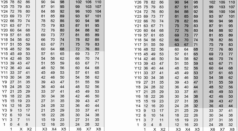
Figure 1: Left part: $X^{\alpha_{1}}Y^{\alpha_{2}}=X^{5}Y^{16}$. Only $B_{1}$ present. Right part: $X^{\alpha_{1}}Y^{\alpha_{2}}=X^{5}Y^{4}$. Light grey area is $B_{1}$, medium grey area is $B_{2}$. $B_{3}$ is not present.

Consider next the case $X^{\alpha_{1}}Y^{\alpha_{2}}=X^{8}Y^{3}$. We have $\alpha_{2}<q-b$ and $\alpha_{1}>a-w(Y)$ and therefore $B_{2}(X^{\alpha_{1}}Y^{\alpha_{2}})$ and $B_{3}(X^{\alpha_{1}}Y^{\alpha_{2}},u)$ for $u=1,2,3$ are non-empty. The situation regarding $B_{2}(X^{\alpha_{1}}Y^{\alpha_{2}})$ is similar to the case $X^{5}Y^{4}$. The set $B_{3}(X^{\alpha_{1}}Y^{\alpha_{2}},u)$ can be thought of as an improvement to $B_{2}(X^{\alpha_{1}}Y^{\alpha_{2}})$. We see that $\gamma_{1}$ runs from $a-w(Y)u$ to $\alpha_{1}$ and $\gamma_{2}$ from $\alpha_{2}+w(X)u$ to $q$. For an illustration see Figure 2.

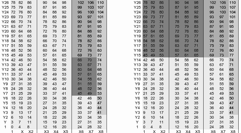
Figure 2: In both parts $X^{\alpha_{1}}Y^{\alpha_{2}}=X^{8}Y^{3}$. Left part: Light grey area is $B_{1}$, medium grey area is $B_{2}$, and dark grey area plus medium grey area correspond to $B_{3}(X^{\alpha_{1}}Y^{\alpha_{2}},1)$. Right part: Light grey area is $B_{1}$, medium grey area is $B_{2}$, and dark grey area plus medium grey area correspond to $B_{3}(X^{\alpha_{1}}Y^{\alpha_{2}},3)$.

Lemma 28.

Consider $\vec{c}={\mbox{ev}}(\sum_{s=1}^{i}a_{s}M_{s}+I_{q})$, $a_{s}\in{\mathbb{F}}_{q}$, $s=1,\ldots,i$, and $a_{i}\neq 0$. Let $M_{i}=X^{\alpha_{1}}Y^{\alpha_{2}}$ and $v=\alpha_{1}{\mbox{ div }}w(Y)$ (that is, $v$ satisfies $\alpha_{1}=w(Y)v+T$, where $T=\alpha_{1}{\mbox{ rem }}w(Y)$). It holds that:

• $B_{1}(X^{\alpha_{1}}Y^{\alpha_{2}})\subseteq{\mathcal{L}}(u)\mbox{ for }u=1,\ldots,v+1$.

• $B_{2}(X^{\alpha_{1}}Y^{\alpha_{2}})\subseteq{\mathcal{L}}(u)\mbox{ for }u=1,\ldots,v+1$.

• $B_{3}(X^{\alpha_{1}}Y^{\alpha_{2}},\gcd(a,b))\subseteq{\mathcal{L}}(v+1)$.

• $B_{3}(X^{\alpha_{1}}Y^{\alpha_{2}},u)\subseteq{\mathcal{L}}(u)\mbox{ for }u=1,\ldots,v$.

Proof.

$B_{1}(X^{\alpha_{1}}Y^{\alpha_{2}})\subseteq{\mathcal{L}}(u)$ for $u=1,\ldots,v+1$:
Assume $M_{l}=X^{\gamma_{1}}Y^{\gamma_{2}}\in B_{1}(X^{\alpha_{1}}Y^{\alpha_{2}})$. We have $\alpha_{1}\leq\gamma_{1}<a$ and $\alpha_{2}\leq\gamma_{2}<q$. Choosing $M_{j}=X^{\gamma_{1}-\alpha_{1}}Y^{\gamma_{2}-\alpha_{2}}$ we get $\mbox{lm}(M_{i}M_{j}{\mbox{ rem }}{\mathcal{G}})=M_{l}$. Let $i^{\prime}\in\{1,\ldots,i-1\}$, then by the properties of a monomial ordering $M_{i^{\prime}}M_{j}\prec_{w}M_{i}M_{j}$ holds. This means that $(M_{i},M_{j})$ is SOWB with respect the set $\{1,\ldots,i\}$. Thus $M_{l}\in{\mathcal{L}}(u)$ for $u=1,\ldots,v+1$.

$B_{2}(X^{\alpha_{1}}Y^{\alpha_{2}})\subseteq{\mathcal{L}}(u)$ for $u=1,\ldots,v+1$:
If $T=0$ or $q-b\leq\alpha_{2}<q$ then the result follows trivially.
Assume $T\neq 0$ and $0\leq\alpha_{2}<q-b$. Let $M_{l}=X^{\gamma_{1}}Y^{\gamma_{2}}\in B_{2}(X^{\alpha_{1}}Y^{\alpha_{2}})$. We have $\alpha_{1}-T\leq\gamma_{1}<\alpha_{1}$ and $\alpha_{2}+b\leq\gamma_{2}<q$. Choosing $M_{j}=X^{\gamma_{1}-\alpha_{1}+a}Y^{\gamma_{2}-\alpha_{2}-b}$ (which belongs to $\Delta_{\prec_{w}}(I_{q})$ by the definition of $B_{2}$) we get

$${\mbox{lm}}(M_{i}M_{j}{\mbox{\ rem\ }}{\mathcal{G}})={\mbox{lm}}(M_{i}M_{j}-X^{\gamma_{1}}Y^{\gamma_{2}-b}F(X,Y))=X^{\gamma_{1}}Y^{\gamma_{2}}.$$

We want to prove that $(M_{i},M_{j})$ is SOWB with respect the set $\{1,\ldots,i\}$. We consider $M_{i^{\prime}}$ with $i^{\prime}\in\{1,\ldots,i-1\}$. If $w(M_{i^{\prime}})<w(M_{i})$ then the proof follows from $w(M_{i^{\prime}}M_{j})<w(M_{i}M_{j})$ using the fact that reducing modulo $F$ does not change the weight of the leading monomial. If $w(M_{i^{\prime}})=w(M_{i})$ then there exists an integer $z$ with $\alpha_{1}-zw(Y)\geq 0$ such that $M_{i^{\prime}}=X^{\alpha_{1}-zw(Y)}Y^{\alpha_{2}+zw(Y)}$. Therefore $\gamma_{1}-zw(Y)\geq 0.$
Now $M_{i^{\prime}}M_{j}=X^{a+\gamma_{1}-zw(Y)}Y^{\gamma_{2}-b+zw(X)}$ and therefore

$${\mbox{lm}}(M_{i^{\prime}}M_{j}{\mbox{ rem }}{\mathcal{G}})={\mbox{lm}}(M_{i^{\prime}}M_{j}-X^{\gamma_{1}-zw(Y)}Y^{\gamma_{2}-b+zw(X)}F(X,Y))$$

$$=X^{\gamma_{1}-zw(Y)}Y^{\gamma_{2}+zw(X)}\prec_{w}X^{\gamma_{1}}Y^{\gamma_{2}}.$$

Again we employed the fact that reducing modulo $F$ does not change the weight of the leading monomial. We conclude that ${\mbox{lm}}(M_{i^{\prime}}M_{j}{\mbox{\ rem\ }}{\mathcal{G}})\prec_{w}X^{\gamma_{1}}Y^{\gamma_{2}}$ and that $(M_{i},M_{j})$ is SOWB with respect the set $\{1,\ldots,i\}$. Thus $M_{l}\in{\mathcal{L}}(u)$ for $u=1,\ldots,v+1$.

$B_{3}(X^{\alpha_{1}}Y^{\alpha_{2}},\gcd(a,b))\subseteq{\mathcal{L}}(v+1)$:
If $0\leq\alpha_{1}\leq a-w(Y)$ or $q-b\leq\alpha_{2}<q$ then the result follows trivially.
Assume $a-w(Y)<\alpha_{1}<a$ and $0\leq\alpha_{2}<q-b$, then $v=\gcd(a,b)-1$. Let $M_{l}=X^{\gamma_{1}}Y^{\gamma_{2}}\in B_{3}(X^{\alpha_{1}}Y^{\alpha_{2}},\gcd(a,b))$. We have $0\leq\gamma_{1}<\alpha_{1}$ and $\alpha_{2}+b\leq\gamma_{2}<q$. Choosing $M_{j}=X^{\gamma_{1}-\alpha_{1}+a}Y^{\gamma_{2}-\alpha_{2}-b}$ we get $\mbox{lm}(M_{i}M_{j}\mbox{ rem }{\mathcal{G}})=M_{l}$. We want to prove that $(M_{i},M_{j})$ is SOWB with respect the set $\{1,\ldots,i-v-1\}$. We consider $M_{i^{\prime}}$ with $i^{\prime}\in\{1,\ldots,i-1\}$. If $w(M_{i^{\prime}})<w(M_{i})$ the proof follows because $w(M_{i^{\prime}}M_{j})<w(M_{i}M_{j})$ using the fact that reducing modulo $F$ does not change the weight of the leading monomial. As $v=\gcd(a,b)-1$ there does not exists any $i^{\prime}\in\{1,\ldots,i-v-1,i\}$ such that $w(M_{i^{\prime}})=w(M_{i})$. From this it follows that $(M_{i},M_{j})$ is SOWB with respect the set $\{1,\ldots,i-v-1\}$ and thus $M_{l}\in{\mathcal{L}}(v+1)$.

$B_{3}(X^{\alpha_{1}}Y^{\alpha_{2}},u)\subseteq{\mathcal{L}}(u)$ for $u=1,\ldots,v$:
If $q-b\leq\alpha_{2}<q$ or $0\leq\alpha_{1}\leq a-w(Y)$ then the result follows trivially.
Assume $a-w(Y)<\alpha_{1}<a$ and $0\leq\alpha_{2}<q-b$, then $v=\gcd(a,b)-1$. Let $M_{l}=X^{\gamma_{1}}Y^{\gamma_{2}}\in B_{3}(X^{\alpha_{1}}Y^{\alpha_{2}},u)$. We have $a-w(Y)u\leq\gamma_{1}<\alpha_{1}$ and $\alpha_{2}+w(X)u\leq\gamma_{2}<q$. By the definition of $\prec_{w}$ and the form of $\Delta_{\prec_{w}}(I_{q})$ we have that $M_{i-u}=X^{\alpha_{1}-w(Y)u}Y^{\alpha_{2}+w(X)u}$. Choosing $M_{j}=X^{\gamma_{1}-\alpha_{1}+w(Y)u}Y^{\gamma_{2}-\alpha_{2}-w(Y)u}$ we get $\mbox{lm}(M_{i-u}M_{j}{\mbox{ rem }}{\mathcal{G}})=M_{l}$. Note that $M_{i-u}$ and $M_{j}$ are in $\Delta_{\prec_{w}}(I_{q})$ because $v=\gcd(a,b)-1$, $a-w(Y)<\alpha_{1}<a$ and $0\leq\alpha_{2}<q-b$. We want to prove that $(M_{i},M_{j})$ is SOWB with respect the set $\{1,\ldots,i-u,i\}$. We consider $M_{i^{\prime}}$ with $i^{\prime}\in\{1,\ldots,i-1\}$. If $w(M_{i^{\prime}})<w(M_{i})$ then the proof follows from $w(M_{i^{\prime}}M_{j})<w(M_{i}M_{j})$ using the fact that reducing modulo $F$ does not change the weight of the leading monomial. The monomials $M_{i^{\prime}}$ which satisfy $w(M_{i^{\prime}})=w(M_{i-u})$ are $M_{i}$ and $M_{i-z}$ for $z=u,\ldots,v$. However, $M_{i}M_{j}{\mbox{ rem }}{\mathcal{G}}\prec_{w}M_{i-u}M_{j}{\mbox{ rem }}{\mathcal{G}}$ because $\gamma_{1}+w(Y)u>a$ and $M_{i-t}M_{j}\prec_{w}M_{i-u}M_{j}$ for any $t=u+1,\ldots,v$ due to the properties of a monomial ordering. From this it follows that $(M_{i},M_{j})$ is SOWB with respect the set $\{1,\ldots,i-u,i\}$ and thus $M_{l}\in{\mathcal{L}}(u)$, for $u=1,\ldots,v$. ∎

Lemma 29.

Consider $\vec{c}={\mbox{ev}}(\sum_{s=1}^{i}a_{s}M_{s}+I_{q})$, $a_{s}\in{\mathbb{F}}_{q}$, $s=1,\ldots,i$, and $a_{i}\neq 0$. Write $M_{i}=X^{\alpha_{1}}Y^{\alpha_{2}}$. For $u=1,\ldots,v+1$, with $v=\alpha_{1}{\mbox{ div }}w(Y)$, we have that:

$$B_{1}(X^{\alpha_{1}}Y^{\alpha_{2}})\cup B_{2}(X^{\alpha_{1}}Y^{\alpha_{2}})\subseteq{\mathcal{L}}(u),$$

$$B_{1}(X^{\alpha_{1}}Y^{\alpha_{2}})\cup B_{3}(X^{\alpha_{1}}Y^{\alpha_{2}},u)\subseteq{\mathcal{L}}(u).$$

Proof.

The lemma follows directly from Remark 27 and Lemma 28. ∎

It is not hard to compute the cardinality of the sets $B_{1}$, $B_{2}$ and $B_{3}$. For $u=1,\ldots,\gcd(a,b)$, we have that:

$$\#B_{1}(X^{\alpha_{1}}Y^{\alpha_{2}})=(a-\alpha_{1})(q-\alpha_{2}),$$

$$\#B_{2}(X^{\alpha_{1}}Y^{\alpha_{2}})=\begin{cases}\alpha_{1}(q-\alpha_{2}-b)&\mbox{ if }0\leq\alpha_{2}<q-b\\ 0&\mbox{ otherwise,}\end{cases}$$

$$\#B_{3}(X^{\alpha_{1}}Y^{\alpha_{2}},u)=\begin{cases}(w(Y)u-a+\alpha_{1})(q-\alpha_{2}-w(X)u)&\mbox{ if }0\leq\alpha_{2}<q-b\mbox{ and }\\ &a-w(Y)<\alpha_{1}<a\\ 0&\mbox{ otherwise.}\end{cases}$$

Thus, for $u=1,\ldots,v+1$ by Lemma 29 we get:

$$\#{\mathcal{L}}(u)\geq(a-\alpha_{1})(q-\alpha_{2})+\begin{cases}\alpha_{1}(q-\alpha_{2}-b)&\mbox{ if }0\leq\alpha_{2}<q-b\\ 0&\mbox{ otherwise}\end{cases}$$

And if $a-w(Y)<\alpha_{1}<a$:

$$\#{\mathcal{L}}(u)\geq(a-\alpha_{1})(q-\alpha_{2})+\begin{cases}(w(Y)u-a+\alpha_{1})(q-\alpha_{2}-w(X)u)&\mbox{ if }0\leq\alpha_{2}<q-b\\ 0&\mbox{ otherwise.}\end{cases}$$

Now we can prove Theorem 25.

Proof of Theorem 25.

Let $v=\alpha_{1}{\mbox{ div }}w(Y)$. If $0\leq\alpha_{1}\leq a-w(Y)$ then we obtain

$$w_{H}(\vec{c}) \geq \min\{\#{\mathcal{L}}(1),\ldots,\#{\mathcal{L}}(v+1)\}$$

$$\geq (a-\alpha_{1})(q-\alpha_{2})+$$

$$\begin{cases}\alpha_{1}(q-\alpha_{2}-b)&\mbox{ if }0\leq\alpha_{2}<q-b\\ 0&\mbox{ otherwise.}\end{cases}$$

If $a-w(Y)<\alpha_{1}<a$, then $v=\gcd(a,b)-1$ and we obtain

$$w_{H}(\vec{c}) \geq \min\{\#{\mathcal{L}}(1),\ldots,\#{\mathcal{L}}(v+1)\}$$

$$\geq (a-\alpha_{1})(q-\alpha_{2})+$$

$$\begin{cases}\min\{(w(Y)u-a+\alpha_{1})(q-\alpha_{2}-w(X)u)\mid u=1,\ldots,v+1\}&\mbox{ if }0\leq\alpha_{2}<q-b\\ 0&\mbox{ otherwise.}\end{cases}$$

The function $f(u)=(w(Y)u-a+\alpha_{1})(q-\alpha_{2}-w(X)u)$ is a concave parabola, thus we have minimum in $u=1$ or $u=v+1=\gcd(a,b)$. By inspection $f(1)=(w(Y)-a+\alpha_{1})(q-\alpha_{2}-w(X))=T(q-\alpha_{2}-w(X))$ and $f(\gcd(a,b))=(w(Y)\gcd(a,b)-a+\alpha_{1})(q-\alpha_{2}-w(X)\gcd(a,b))=\alpha_{1}(q-\alpha_{2}-b)$. We therefore get the biimplication:

$$f(1)\leq f(\gcd(a,b)),$$

$$\Updownarrow$$

$$\alpha_{2}\leq q-w(X)-\alpha_{1}\frac{b-w(X)}{a-w(Y)},$$

and the theorem follows. ∎

Remark 30.

If for codes from optimal generalised $C_{ab}$ polynomials rather than applying Theorem 13 we apply the usual Feng-Rao bound (Theorem 8) then the $\epsilon$ in Theorem 25 should be replaced with:

$$\begin{cases}0&\mbox{if }q-b\leq\alpha_{2}<q\\ T(q-\alpha_{2}-b)&\mbox{and }0\leq\alpha_{2}<q-b.\\ \end{cases}$$

We see that our new bound improves the Feng-Rao bound by

$$\begin{cases}0&\mbox{if }q-b\leq\alpha_{2}<q\\ &\mbox{or }0\leq\alpha_{1}\leq a-w(Y)\\ (\alpha_{1}-T)(q-\alpha_{2}-b)&\mbox{if }a-w(Y)<\alpha_{1}<a\mbox{ and }\\ &q-w(X)-\alpha_{1}\frac{b-w(X)}{a-w(Y)}<\alpha_{2}<q-b\\ T(b-w(X))&\mbox{if }a-w(Y)<\alpha_{1}<a\mbox{ and }\\ &0\leq\alpha_{2}\leq q-w(X)-\alpha_{1}\frac{b-w(X)}{a-w(Y)}.\end{cases}$$

Remark 31.

It is possible to show that Theorem 25 is the strongest possible result one can derive from Theorem 13 regarding the minimum distance of codes from optimal generalised $C_{ab}$ polynomials.

In the following we apply Theorem 25 in a number of cases where $F(X,Y)=G(X)-H(Y)\in{\mathbb{F}}_{p^{m}}[X,Y]$ with $G(X)$ being the trace polynomial and $H(Y)$ being an $({\mathbb{F}}_{p^{m}},{\mathbb{F}}_{p})$-polynomial of another degree. Recall from the discussion at the beginning of the section that these are optimal generalised $C_{ab}$ polynomials. The strength of our new bound Theorem 13 and Theorem 25 lies in the cases where $a$ and $b$ are not relatively prime, as for $a$ and $b$ relatively prime it reduces to the usual Feng-Rao bound for primary codes (see the last part of Remark 14). The well-known norm-trace polynomial corresponds to choosing $H(Y)$ to be the norm polynomial. This gives $a=p^{m-1}$ and $b=(p^{m}-1)/(p-1)$ which are clearly relatively prime. The related codes, which are called norm-trace codes, are one-point algebraic geometric codes. As a measure for how good is our new code constructions it seems fair to compare the outcome of Theorem 25 for the cases of $\gcd(a,b)>1$ with the parameters of the one-point algebraic geometric codes from norm-trace curves over the same alphabet. The two corresponding sets of ideals have the same footprint $\Delta_{\prec_{w}}(I_{q})$ and consequently the corresponding codes are of the same length. We remind the reader that it was shown in [5] that the Feng-Rao bound gives the true parameters of the norm-trace codes.

Example 5.

In this example we consider optimal generalised $C_{ab}$ polynomials derived from $({\mathbb{F}}_{8},{\mathbb{F}}_{2})$-polynomials. The trace polynomial $G(X)$ is of degree $a=4$ and from Example 3 we see that besides the norm polynomial which is of degree $b=7$ we can choose $H(Y)$ as $F_{3}(Y)=Y^{6}+Y^{5}+Y^{3}$ which is of degree $b=6$. The corresponding codes are of length $n=32$ over the alphabet ${\mathbb{F}}_{8}$. In Figure 3 below we compare the parameters of the related two sequences of improved codes $\widetilde{E}_{imp}(\delta)$ (Definition 15). For few choices of $\delta$ the norm-trace code is the best, but for many choices of $\delta$, from $(a,b)=(4,6)$ we get better codes. We note that the latter sequence of codes contains two non-trivial codes that has the best known parameters according to the linear code bound at [11], namely $[n,k,d]$ equal to $[32,2,28]$ and $[32,15,12]$.

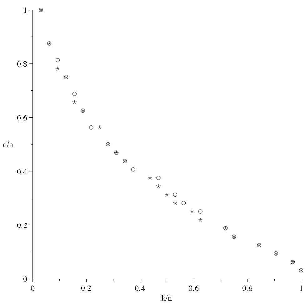
Figure 3: Improved codes from Example 5. A $\circ$ corresponds to $(a,b)=(4,6)$, and an $\ast$ corresponds to $(a,b)=(4,7)$ (the norm-trace codes).

Example 6.

In this example we consider optimal generalised $C_{ab}$ polynomials derived from $({\mathbb{F}}_{16},{\mathbb{F}}_{2})$-polynomials. The trace polynomial $G(X)$ is of degree $a=8$ and from Example 3 we see that besides the norm polynomial which is of degree $b=15$ we can choose $H(Y)$ to be of degree $10$, $12$ and $14$. The corresponding codes are of length $n=128$ over the alphabet ${\mathbb{F}}_{16}$. In Figure 4 below we compare the parameters of the related two sequences of improved codes $\widetilde{E}_{imp}(\delta)$ when $b=10$ and when $b=15$ (the norm-trace codes). For most choices of $\delta$ from $(a,b)=(8,10)$ we get the best codes. The norm-trace codes are never strictly best.

Figure 4: Improved codes from Example 6. A $\circ$ corresponds to $(a,b)=(8,10)$, and an $\ast$ corresponds to $(a,b)=(8,15)$ (the norm-trace codes).

Example 7.

In this example we consider optimal generalised $C_{ab}$ polynomials derived from $({\mathbb{F}}_{32},{\mathbb{F}}_{2})$-polynomials. The trace polynomial $G(X)$ is of degree $a=16$ and from Example 3 we see that besides the norm-polynomial which is of degree $b=31$ we can choose $H(Y)$ to be of degree $20$, $24$, $26$, $28$ and $30$. The corresponding codes are of length $n=512$ over the alphabet ${\mathbb{F}}_{32}$. In Figure 5 below we compare the parameters of the related three sequences of improved codes $\widetilde{E}_{imp}(\delta)$ when $b=20$, $b=26$ and when $b=31$ (the norm-trace codes). For no choices of $\delta$ the norm-trace codes are strictly best (this holds for all values of $k/n$). For some choices $b=20$ gives the best codes for other choices the best parameters are found by choosing $b=26$.

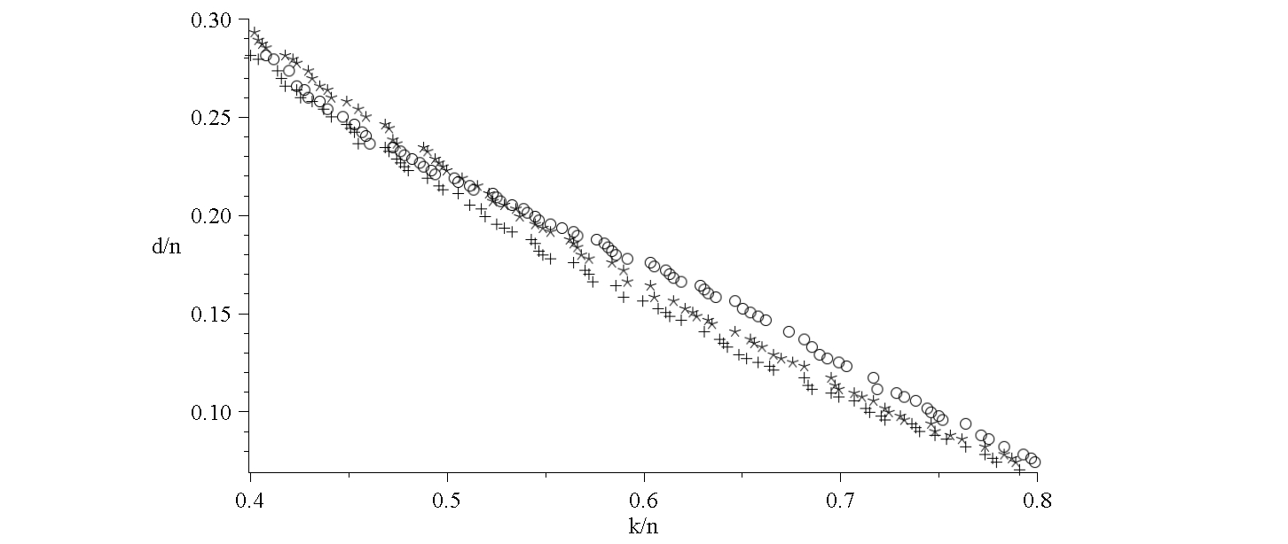
Figure 5: Improved codes from Example 7. A $\circ$ corresponds to $(a,b)=(16,20)$, an $\ast$ to $(a,b)=(16,26)$, and finally a $+$ corresponds to $(a,b)=(16,31)$ (the norm-trace codes).

Example 8.

In this example we consider optimal generalised $C_{ab}$ polynomials derived from $({\mathbb{F}}_{64},{\mathbb{F}}_{2})$-polynomials. The trace polynomial $G(X)$ is of degree $a=32$ and by studying cyclotomic cosets we see that as an alternative to the norm polynomial which is of degree $b=63$ we can for instance choose an $H(Y)$ of degree $42$. The corresponding codes are of length $n=2048$ over the alphabet ${\mathbb{F}}_{64}$. In Figure 6 below we compare the parameters of the related two sequences of improved codes $\widetilde{E}_{imp}(\delta)$ when $b=42$ and when $b=63$ (the norm-trace codes). As is seen the first codes outperforms the last codes for all parameters.

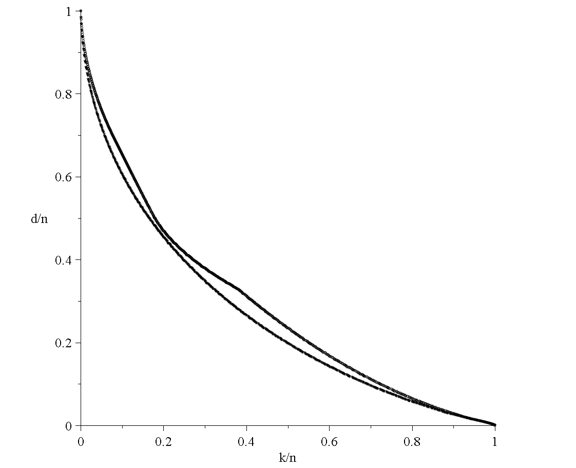
Figure 6: Improved codes from Example 8. The upper curve corresponds to $(a,b)=(32,42)$, the lower curve to $(a,b)=(32,63)$ (the norm-trace codes)

5 A new construction of improved codes

In Definition 15 we presented a Feng-Rao style improved code construction $\widetilde{E}_{imp}(\delta)$. As shall be demonstrated in this section it is sometimes possible to do even better. Recall that the idea behind Theorem 13 is to consider case 1 up till case v+1 as described prior to the theorem. Consider a general codeword

$$\vec{c}={\mbox{ev}}\big{(}\sum_{s=1}^{i}a_{s}M_{s}+I_{q}\big{)}\in C(I,L)$$

$a_{i}\neq 0$, where $L$ is some fixed known subspace of ${\mathbb{F}}_{q}^{n}$. From $L$ we might a priori be able to conclude that certain $a_{s}$s equal zero for all codewords as above. This corresponds to saying that a priori we might know that some of the cases case 1 up to case v do not happen. Clearly we could then leave out the corresponding sets in Theorem 13. This might result in a higher estimate on $w_{H}(\vec{c})$. We illustrate the phenomenon with an example in which we also show how to derive improved codes based on this observation.

Example 9.

In this example we consider the Klein quartic $X^{3}Y+Y^{3}+X\in{\mathbb{F}}_{8}[X,Y]$. Let $w(X)=2$ and $w(Y)=3$. The ideal $I=\langle X^{3}Y+Y^{3}+X\rangle\subseteq{\mathbb{F}}_{8}[X,Y]$ and the corresponding weighted degree lexicographic ordering $\prec_{w}$ satisfy order domain condition (C1) but not (C2) (as usual, in the definition of $\prec_{w}$ we choose $X=X_{1}$ and $Y=X_{2}$). Hence, it makes sense to apply Theorem 13. The footprint of $I_{8}=\langle X^{3}Y+Y^{3}+X,X^{8}+X,Y^{8}+Y\rangle$ is (for a reference see [6, Ex. 4.19] and [3, Ex. 3.3]):

$$\Delta_{\prec_{w}}(I_{8}) = \{1,X,Y,X^{2},XY,Y^{2},X^{3},X^{2}Y,XY^{2},X^{4},Y^{3},X^{2}Y^{2},$$

$$X^{5},XY^{3},Y^{4},X^{6},X^{2}Y^{3},XY^{4},X^{7},Y^{5},X^{2}Y^{4},Y^{6}\}$$

written in increasing order with respect to $\prec_{w}$. Consider

$$\vec{c}={\mbox{ev}}\big{(}a_{1}1+a_{2}X+a_{3}Y+a_{4}X^{2}+a_{5}XY+a_{6}Y^{2}+a_{7}X^{3}+I_{8}\big{)},$$

$a_{7}\neq 0$. We have $w(X^{3})=w(Y^{2})>w(XY)$. Hence, by Remark 14 we choose $v=1$.
By inspection the set corresponding to case 1 is

$${\mathcal{L}}(1)=\{X^{3},X^{4},X^{5},X^{6},X^{7},X^{2}Y^{4}\}.$$

(Note that $X^{2}Y^{4}$ belongs to ${\mathcal{L}}(1)$ of the following reason: We have ${\mbox{lm}}(X^{3}X^{5}{\mbox{ rem }}X^{8}+X)=X$ and ${\mbox{lm}}(Y^{2}X^{5}{\mbox{ rem }}X^{3}Y+Y^{3}+X)=X^{2}Y^{4}$, and from $w(Y^{2}X^{5})=w(X^{2}Y^{4})>w(X)$ we conclude that $(Y^{2},X^{5})$ is SOWB with respect to $\{1,2,3,4,5,6,7\}$.) The set corresponding to case 2 is

$${\mathcal{L}}(2)=\{X^{3},X^{4},Y^{3},X^{5},XY^{3},Y^{4},X^{6},X^{2}Y^{3},XY^{4},X^{7},Y^{5},X^{2}Y^{4},Y^{6}\}.$$

If we know a priori that $a_{6}=0$ then we can conclude from the above that $w_{H}(\vec{c})\geq\#{\mathcal{L}}(2)=13$. Without such an information we can only conclude

$$w_{H}(\vec{c})\geq\min\{\#{\mathcal{L}}(1),\#{\mathcal{L}}(2)\}=6.$$

It can be shown using Theorem 13 that $\widetilde{E}_{imp}(11)=C(I,L)$ where

$$L={\mbox{ev}}\big{(}{\mbox{Span}}_{\mathbb{F}_{8}}\{1+I_{8},X+I_{8},Y+I_{8},X^{2}+I_{8},XY+I_{8},Y^{2}+I_{8}\}\big{)}.$$

That is, a code with parameters $[n,k,d]$ equal to $[22,6,\geq 11]$.
If instead we choose

$$\widetilde{L}={\mbox{ev}}\big{(}{\mbox{Span}}_{\mathbb{F}_{8}}\{1+I_{8},X+I_{8},Y+I_{8},X^{2}+I_{8},XY+I_{8},X^{3}+I_{8}\}\big{)}$$

then we do not need to consider the case 1 described above. By inspection the code parameters $[n,k,d]$ of $C(I,\widetilde{L})$ are $[22,6,\geq 12]$.

6 Generalised Hamming weights

As mentioned at the end of Section 2 it is possible to lift Theorem 13 to also deal with generalised Hamming weights. Recall that these parameters are important in the analysis of the wiretap channel of type II as well as in the analysis of secret sharing schemes based on coding theory, see [23], [15] and [14].

Definition 32.

Let $C\subseteq{\mathbb{F}}_{q}^{n}$ be a code of dimension $k$. For $t=1,\ldots,k$ the $t$th generalised Hamming weight is

$$d_{t}(C)=\min\{\#{\mbox{Supp}}\,D\mid D{\mbox{ \ is a subspace of \ }}C{\mbox{ \ of dimension \ }}t\}.$$

Here, ${\mbox{Supp}}\,D$ means the entries for which some word in $D$ is different from zero.

Clearly, $d_{1}$ is nothing but the usual minimum distance. In Proposition 33 below we lift Theorem 13 to deal with the second generalised Hamming weight. From this the reader can understand how to treat any generalised Hamming weight.

Proposition 33.

Let $D\subseteq{\mathbb{F}}_{q}^{n}$ be a subspace of dimension 2. Write $D={\mbox{Span}}_{\mathbb{F}_{q}}\{{\mbox{ev}}(\sum_{s=0}^{i_{1}}a_{s}M_{s}),{\mbox{ev}}(\sum_{s=0}^{i_{2}}b_{s}M_{s})\}$. Here, $\Delta_{\prec}(I_{q})=\{M_{1},\ldots,M_{n}\}$, $a_{s}\in{\mathbb{F}}_{q}$, $b_{s}\in{\mathbb{F}}_{q}$ with $a_{i_{1}}\neq 0$ and $b_{i_{2}}\neq 0$. Without loss of generality we may assume $i_{1}\neq i_{2}$. Let $v_{1}$ and $v_{2}$ be integers satisfying $0\leq v_{1}<i_{1}$ and $0\leq v_{2}<i_{2}$. We have

$$\#{\mbox{Supp}}(D)\geq\min\{\#{\mathcal{L}}(z_{1},z_{2})\mid 1\leq z_{1}\leq v_{1}+1,1\leq z_{2}\leq v_{2}+1\}.$$

The above sets are defined as follows: For $z=1,\ldots,v_{1}$

$${\mathcal{L}}(z,v_{2}+1)=$$

$$\big{\{}K\in\Delta_{\prec}(I_{q})\mid\exists M_{j}\in\Delta_{\prec}(I_{q}){\mbox{ such that either }}(M_{i_{1}},M_{j}){\mbox{ is SOWB}}$$

$${\mbox{ with respect to }}\{1,\ldots,i_{1}-z,i_{1}\}{\mbox{ and }}{\mbox{lm}}(M_{i_{1}}M_{j}{\mbox{ rem }}{\mathcal{G}})=K$$

or

$$(M_{i_{1}-z},M_{j}){\mbox{ is SOWB with respect to }}\{1,\ldots,i_{1}-z,i_{1}\}$$

$${\mbox{ and }}{\mbox{lm}}(M_{i_{1}-z}M_{j}{\mbox{ rem }}{\mathcal{G}})=K$$

or

$$(M_{i_{2}},M_{j}){\mbox{ is SOWB with respect to }}\{1,\ldots,i_{2}-v_{2}-1\}$$

$${\mbox{ and }}{\mbox{lm}}(M_{i_{2}}M_{j}{\mbox{ rem }}{\mathcal{G}})=K\big{\}}.$$

For $z=1,\ldots,v_{2}$, ${\mathcal{L}}(v_{1}+1,z)$ is defined in a similar way.
For $z_{1}=1,\ldots,v_{1}$ and $z_{2}=1,\ldots,v_{2}$ we have

$${\mathcal{L}}(z_{1},z_{2})=$$

$$\big{\{}K\in\Delta_{\prec}(I_{q})\mid\exists M_{j}\in\Delta_{\prec}(I_{q}){\mbox{ such that for some $u\in\{1,2\}$}}$$

$$(M_{i_{u}},M_{j}){\mbox{ is SOWB with respect to }}\{1,\ldots,i_{u}-z_{u},i_{u}\}$$

$${\mbox{ and }}{\mbox{lm}}(M_{i_{u}}M_{j}{\mbox{ rem }}{\mathcal{G}})=K$$

or

$$(M_{i_{u}-z_{u}},M_{j}){\mbox{ is SOWB with respect to }}\{1,\ldots,i_{u}-z_{u},i_{u}\}$$

$${\mbox{ and }}{\mbox{lm}}(M_{i_{u}-z_{u}}M_{j}{\mbox{ rem }}{\mathcal{G}})=K\big{\}},$$

and finally

$${\mathcal{L}}(v_{1}+1,v_{2}+1)=$$

$$\big{\{}K\in\Delta_{\prec}(I_{q})\mid\exists M_{j}\in\Delta_{\prec}(I_{q}){\mbox{ such that }}(M_{i_{u}},M_{j}){\mbox{ is SOWB}}$$

$${\mbox{ with respect to }}\{1,\ldots,i_{u}-v_{u}-1\}{\mbox{ and }}{\mbox{lm}}(M_{i_{u}}M_{j}{\mbox{ rem }}{\mathcal{G}})=K$$

$${\mbox{ for some }}u\in\{1,2\}\big{\}}.$$

The second generalised Hamming weight of $C(I,L)$ is found by repeating the above process for all possible choices of $i_{1}<i_{2}$ corresponding to the cases that $D\subseteq C(I,L)$.

Proof.

The proof is a straight forward enhancement of the proof for Theorem 13.

∎

For the choice of $v_{1}$ and $v_{2}$ in Proposition 33 we refer to Remark 14. Admittedly, the proposition is rather technical. Nevertheless even its generalisation to higher generalised Hamming weights can often be quite manageable. We shall comment further on this in Section 9.

7 Formulation at linear code level

As mentioned in the introduction the Feng-Rao bound for primary codes in its most general form is a bound on any linear code described by means of a generator matrix. All other versions of the bound, such as the order bound for primary codes and the Feng-Rao bound for primary affine variety codes, can be viewed as corollaries to it. Below we reformulate the new bound in Theorem 13 at the linear code level.
Let $n$ be a positive integer and $q$ a prime power. Consider a fixed ordered triple $({\mathcal{U}},{\mathcal{V}},{\mathcal{W}})$ where ${\mathcal{U}}=\{\vec{u}_{1},\ldots,\vec{u}_{n}\}$, ${\mathcal{V}}=\{\vec{v}_{1},\ldots,\vec{v}_{n}\}$, and ${\mathcal{W}}=\{\vec{w}_{1},\ldots,\vec{w}_{n}\}$ are three (possibly different) bases for ${\mathbb{F}}_{q}^{n}$ as a vector space over ${\mathbb{F}}_{q}$. We shall always denote by ${\mathcal{I}}$ the set $\{1,\ldots,n\}$.

Definition 34.

Consider a basis ${\mathcal{A}}=\{\vec{a}_{1},\ldots,\vec{a}_{n}\}$ for ${\mathbb{F}}_{q}^{n}$ as a vector space over ${\mathbb{F}}_{q}$. We define a function $\bar{\rho}_{\mathcal{A}}:{\mathbb{F}}_{q}^{n}\rightarrow\{0,1,\ldots,n\}$ as follows. For $\vec{c}\in{\mathbb{F}}_{q}\backslash\{\vec{0}\}$ we let $\bar{\rho}_{\mathcal{A}}(\vec{c})=i$ if $\vec{c}\in{\mbox{Span}}_{\mathbb{F}_{q}}\{\vec{a}_{1},\ldots,\vec{a}_{i}\}\backslash{\mbox{Span}}_{\mathbb{F}_{q}}\{\vec{a}_{1},\ldots,\vec{a}_{i-1}\}$. Here, we used the notion ${\mbox{Span}}_{\mathbb{F}_{q}}\,\emptyset=\{\vec{0}\}$. Finally, we let $\bar{\rho}_{\mathcal{A}}(\vec{0})=0$.

The component wise product plays a crucial role in the linear code enhancement of Theorem 13.

Definition 35.

The component wise product of two vectors $\vec{u}$ and $\vec{v}$ in ${\mathbb{F}}_{q}^{n}$ is defined by $(u_{1},\ldots,u_{n})\ast(v_{1},\ldots,v_{n})=(u_{1}v_{1},\ldots,u_{n}v_{n})$.

Definition 36.

Let $({\mathcal{U}},{\mathcal{V}},{\mathcal{W}})$ and ${\mathcal{I}}$ be as above. Consider ${\mathcal{I}}^{\prime}\subseteq{\mathcal{I}}$. An ordered pair $(i,j)\subseteq{\mathcal{I}}^{\prime}\times{\mathcal{I}}$ is said to be one-way well-behaving (OWB) with respect to ${\mathcal{I}}^{\prime}$ if $\bar{\rho}_{\mathcal{W}}(\vec{u}_{i^{\prime}}\ast\vec{v}_{j})<\bar{\rho}_{\mathcal{W}}(\vec{u}_{i}\ast\vec{v}_{j})$ holds for all $i^{\prime}\in{\mathcal{I}}^{\prime}$ with $i^{\prime}<i$.

The following theorem is a first generalisation of the Feng-Rao bound for primary codes. The generalisation compared to the usual Feng-Rao bound [1, 10] is that we allow ${\mathcal{I}}^{\prime}$ to be different from $\{1,\ldots,\#{\mathcal{I}}^{\prime}\}$. This is in the spirit of Section 5.

Theorem 37.

Consider $\vec{c}=\sum_{s=1}^{t}a_{s}\vec{u}_{i_{s}}$ with $a_{s}\in{\mathbb{F}}_{q}$, $s=1,\ldots,t$, $a_{t}\neq 0$ and $i_{1}<\cdots<i_{t}$. We have

$$\begin{array}[]{r}w_{H}(\vec{c})\geq\#\big{\{}l\in{\mathcal{I}}\mid\exists j\in{\mathcal{I}}{\mbox{ \ such that \ }}\bar{\rho}_{\mathcal{W}}(\vec{u}_{i_{t}}\ast\vec{v}_{j})=l,{\mbox{ \ \hskip 28.45274pt \ }}\\ (i_{t},j){\mbox{ \ is OWB with respect to \ }}\{i_{1},\ldots,i_{t}\}\big{\}}.\end{array}$$ (6)

Proof.

Let $l_{1}<\cdots<l_{\sigma}$ be the indexes $l$ counted in (6). Denote by $j_{1},\ldots,j_{\sigma}$ the corresponding $j$-values from (6). By assumption $\vec{c}\ast\vec{v}_{j_{1}},\ldots,\vec{c}\ast\vec{v}_{j_{\sigma}}$ are linearly independent and therefore

$${\mbox{Span}}_{\mathbb{F}_{q}}\{\vec{c}\ast\vec{v}_{j_{1}},\ldots,\vec{c}\ast\vec{v}_{j_{\sigma}}\}=\vec{c}\ast{\mbox{Span}}_{\mathbb{F}_{q}}\{\vec{v}_{j_{1}},\ldots,\vec{v}_{j_{\sigma}}\}$$

is a vector space of dimension $\sigma$. The theorem follows from the fact that $\vec{c}\ast{\mathbb{F}}_{q}^{n}$ is a vector space of dimension $w_{H}(\vec{c})$ containing the above space. ∎

A slight modification of Definition 36 and the above proof allows for further improvements.

Definition 38.

Let ${\mathcal{I}}^{\prime}\subseteq{\mathcal{I}}$. A pair $(i,j)\in{\mathcal{I}}^{\prime}\times{\mathcal{I}}$ is called strongly one-way well-behaving (SOWB) with respect to ${\mathcal{I}}^{\prime}$ if $\bar{\rho}_{\mathcal{W}}(\vec{u}_{i^{\prime}}\ast\vec{v}_{j})<\bar{\rho}_{\mathcal{W}}(\vec{u}_{i}\ast\vec{v}_{j})$ holds for all $i^{\prime}\in{\mathcal{I}}^{\prime}\backslash\{i\}$.

The following theorem is the linear code interpretation of Theorem 13. Besides working for a larger class of codes, it is slightly stronger in that we formulate it in such a way that it supports the technique explained in Section 5. Concretely, what makes it stronger than Theorem 13 is the presence of the set $\hat{\mathcal{I}}$.

Theorem 39.

Consider a non-zero codeword $\vec{c}=\sum_{t=1}^{i}a_{t}\vec{u}_{t}$, $a_{t}\in{\mathbb{F}}_{q}$ for $t=1,\ldots,i$, $a_{i}\neq 0$. Let $v$ be an integer $0\leq v<i$. Assume that for some set $\hat{\mathcal{I}}\subseteq\{1,\ldots,i-1\}$ we know a priori that $a_{x}=0$ when $x\in\hat{\mathcal{I}}$. Let $z_{1}<\cdots<z_{s}$ be the numbers in $\{z\in\{i-v,\ldots,i-1\}\mid z\notin\hat{\mathcal{I}}\}$. Write ${\mathcal{I}}^{\ast}=\{z\in\{1,\ldots,i-v-1\}\mid z\notin\hat{\mathcal{I}}\}$. We have

$$w_{H}(\vec{c})\geq\min\{{\mathcal{L}}^{\prime}(1),\ldots,{\mathcal{L}}^{\prime}(s+1)\}$$

where for $t=1,\ldots,s$ we define ${\mathcal{L}}^{\prime}(t)$ as follows:

$${\mathcal{L}}^{\prime}(1) = \{l\in{\mathcal{I}}\mid\exists z\in\{z_{s},i\}{\mbox{ \ and \ }}j\in{\mathcal{I}}{\mbox{ \ such that \ }}\bar{\rho}_{\mathcal{W}}(\vec{u}_{z}\ast\vec{v_{j}})=l$$

$$(z,j){\mbox{ \ is SOWB with respect to \ }}{\mathcal{I}}^{\ast}\cup\{z_{1},\ldots,z_{s},i\}\big{\}},$$

$${\mathcal{L}}^{\prime}(2) = \big{\{}l\in{\mathcal{I}}\mid\exists z\in\{z_{s-1},i\}{\mbox{ \ and \ }}j\in{\mathcal{I}}{\mbox{ \ such that \ }}\bar{\rho}_{\mathcal{W}}(\vec{u}_{z}\ast\vec{v}_{j})=l$$

$$(z,j){\mbox{ \ is SOWB with respect to \ }}{\mathcal{I}}^{\ast}\cup\{z_{1},\ldots,z_{s-1},i\}\big{\}},$$

$${\mbox{ \ {\hskip 85.35826pt }}}\vdots$$

$${\mathcal{L}}^{\prime}(s) = \big{\{}l\in{\mathcal{I}}\mid\exists z\in\{z_{1},i\}{\mbox{ \ and \ }}j\in{\mathcal{I}}{\mbox{ \ such that \ }}\bar{\rho}_{\mathcal{W}}(\vec{u}_{z}\ast\vec{v}_{j})=l$$

$$(z,j){\mbox{ \ is SOWB with respect to \ }}{\mathcal{I}}^{\ast}\cup\{z_{1},i\}\big{\}}.$$

Finally,

$${\mathcal{L}}^{\prime}(s+1) = \big{\{}l\in{\mathcal{I}}\mid\exists j\in{\mathcal{I}}{\mbox{ \ such that \ }}\bar{\rho}_{\mathcal{W}}(\vec{u}_{i}\ast\vec{v}_{j})=l$$

$$(i,j){\mbox{ \ is OWB with respect to \ }}{\mathcal{I}}^{\ast}\cup\{i\}\big{\}}.$$

To establish a lower bound on the minimum distance of a code $C$ we repeat the above process for each $i\in\bar{\rho}_{\mathcal{U}}(C)$. For each such $i$ we choose a corresponding $v$, defining an $s$, and we determine the sets ${\mathcal{L}}^{\prime}(1),\ldots,{\mathcal{L}}^{\prime}(s+1)$ and calculate their cardinalities. The smallest cardinality found when $i$ runs through $\bar{\rho}_{\mathcal{U}}(C)$ serves as a lower bound on the minimum distance.

Proof.

The proof is a direct translation of the proof of Theorem 13. ∎

Remark 40.

For $v=0$ Theorem 39 reduces to Theorem 37. For higher values of $v$ Theorem 39 is at least as strong as Theorem 37 and sometimes stronger. In the same way as Theorem 13 was lifted in Section 6 to deal with generalised Hamming weights one can lift Theorem 37 and Theorem 39.

8 A related bound for dual codes

In the recent paper [8] we presented a new bound for dual codes. This bound is an improvement to the Feng-Rao bound for such codes as well as an improvement to the advisory bound from [22]. The new bound of the present paper can be viewed as a natural counter part to the bound from [8], the one bound dealing with primary codes and the other with dual codes.

Definition 41.

Consider an ordered triple of bases $({\mathcal{U}},{\mathcal{V}},{\mathcal{W}})$ for ${\mathbb{F}}_{q}^{n}$ and ${\mathcal{I}}$ as in Section 7. We define $m:{\mathbb{F}}_{q}^{n}\backslash\{\vec{0}\}\rightarrow{\mathcal{I}}$ by $m(\vec{c})=l$ if $l$ is the smallest number in ${\mathcal{I}}$ for which $\vec{c}\cdot\vec{w}_{l}\neq 0$. (Here, and in the following the symbol $\cdot$ means the usual inner product).

Definition 42.

Consider numbers $1\leq l,l+1,\ldots,l+g\leq n$. A set ${\mathcal{I}}^{\prime}\subseteq{\mathcal{I}}$ is said to have the $\mu$-property with respect to $l$ with exception $\{l+1,\ldots,l+g\}$ if for all $i\in{\mathcal{I}}^{\prime}$ a $j\in{\mathcal{I}}$ exists such that

• $\bar{\rho}_{\mathcal{W}}(\vec{u}_{i}\ast\vec{v}_{j})=l$, and

• for all $i^{\prime}\in{\mathcal{I}}^{\prime}$ with $i^{\prime}<i$ either $\bar{\rho}_{\mathcal{W}}(\vec{u}_{i^{\prime}}\ast\vec{v}_{j})<l$ or $\bar{\rho}_{\mathcal{W}}(\vec{u}_{i^{\prime}}\ast\vec{v}_{j})\in\{l+1,\ldots,l+g\}$ holds.

Assume next that $l+g+1\leq n$. The set ${\mathcal{I}}^{\prime}$ is said to have the relaxed $\mu$-property with respect to $(l,l+g+1)$ with exception $\{l+1,\ldots,l+g\}$ if for all $i\in{\mathcal{I}}^{\prime}$ a $j\in{\mathcal{I}}$ exists such that either conditions $(1a)$ and $(1b)$ above hold or

• $\bar{\rho}_{\mathcal{W}}(\vec{u}_{i}\ast\vec{v}_{j})=l+g+1$, and

• $(i,j)$ is OWB with respect to ${\mathcal{I}}^{\prime}$, and

• no $i^{\prime}\in{\mathcal{I}}^{\prime}$ with $i^{\prime}<i$ satisfies $\bar{\rho}_{\mathcal{W}}(\vec{u}_{i^{\prime}}\ast\vec{v}_{j})=l$.

The new bound from [8, Th. 19] reads:

Theorem 43.

Consider a non-zero codeword $\vec{c}$ and let $l=m(\vec{c})$. Choose a non-negative integer $v$ such that $l+v\leq n$. Assume that for some indexes $x\in\{l+1,\ldots,l+v\}$ we know a priori that $\vec{c}\cdot\vec{w}_{x}=0$. Let $l^{\prime}_{1}<\cdots<l^{\prime}_{s}$ be the remaining indexes from $\{l+1,\ldots,l+v\}$. Consider the sets ${\mathcal{I}}^{\prime}_{0},{\mathcal{I}}_{1}^{\prime},\ldots,{\mathcal{I}}_{s}^{\prime}$ such that:

• ${\mathcal{I}}^{\prime}_{0}$ has the $\mu$-property with respect to $l$ with exception $\{l+1,\ldots,l+v\}$.

• For $i=1,\ldots,s$, ${\mathcal{I}}^{\prime}_{i}$ has the relaxed $\mu$-property with respect to $(l,l^{\prime}_{i})$ with exception $\{l+1,\ldots,l^{\prime}_{i}-1\}$.

We have

$$w_{H}(\vec{c})\geq\min\{\#{\mathcal{I}}_{0}^{\prime},\#{\mathcal{I}}_{1}^{\prime},\ldots,\#{\mathcal{I}}_{s}^{\prime}\}.$$ (7)

To establish a lower bound on the minimum distance of a code $C$ we repeat the above process for each $l\in m(C)$. For each such $l$ we choose a corresponding $v$, we determine sets ${\mathcal{I}}^{\prime}_{i}$ as above and we calculate the right side of (7). The smallest value found when $l$ runs through $m(C)$ constitutes a lower bound on the minimum distance.

If we compare Theorem 43 with Theorem 39 we see that to some extend they have the same flavor. Besides that one deals with dual codes and the other with primary codes another difference is that we in Theorem 43 has the freedom to choose appropriate sets ${\mathcal{I}}^{\prime}_{0},\ldots,{\mathcal{I}}^{\prime}_{s}$ whereas the sets ${\mathcal{L}}^{\prime}(1),\ldots,{\mathcal{L}}^{\prime}(s+1)$ in Theorem 39 are unique. In [8] it was also shown how to lift Theorem 43 to deal with generalised Hamming weights. Similar remarks as above hold for the two bounds when applied to such parameters.

9 A comparison of the new bounds for primary and dual codes

Recall that it was shown in [9] how the Feng-Rao bound for primary codes and the Feng-Rao bound for dual codes can be viewed as consequences of each other. This result holds when the bound is equipped with one of the well-behaving properties WB or OWB. Regarding the case where WWB is used a possible connection is unknown. In a similar fashion as the proof in [9] breaks down if one uses WWB it also breaks down when one tries to prove a correspondence between Theorem 39 and Theorem 43. We leave it as an open research problem to decide if a general connection exists or not.
In Section 4 we analysed the performance of primary affine variety codes coming from optimal generalised $C_{ab}$ polynomials. Using the method from Section 8 one can make a similar analysis for the corresponding dual codes producing similar code parameters. As an alternative, below we explain how to derive this result directly from what we have already shown regarding primary codes from optimal generalised $C_{ab}$ polynomials.
Recall that for optimal generalised $C_{ab}$ polynomials $\Delta_{\prec_{w}}(I_{q})$ is a box:

$$\Delta_{\prec_{w}}(I_{q})=\{M_{1},\ldots,M_{n}\}=\{X^{\alpha_{1}}Y^{\alpha_{2}}\mid 0\leq\alpha_{1}<a,0\leq\alpha_{2}<q\}.$$

This fact gives us the following crucial implication (as usual we assume $M_{1}\prec_{w}\cdots\prec_{w}M_{n}$):

$$M_{i}=X^{\alpha_{1}}Y^{\alpha_{2}}\Rightarrow M_{n-i+1}=X^{a-1-\alpha_{1}}Y^{q-1-\alpha_{2}},{\mbox{ for }}i=1,\ldots,n.$$ (8)

Consider codewords $\vec{c}={\mbox{ev}}\big{(}\sum_{s=1}^{i}a_{s}M_{s}+I_{q}\big{)}$, $a_{s}\in{\mathbb{F}}_{q}$, $a_{i}\neq 0$, and $\vec{c}^{\prime}\in{\mathbb{F}}_{q}^{n}$ such that $m(\vec{c}^{\prime})=n-i+1$. Let $v$ be an integer, $0\leq v<i$. Recall that in Section 4 we determined ${\mathcal{L}}(u)$, $u=1,\ldots,v+1$. If we use Theorem 43 with $\{l+1,\ldots,l+v\}=\{l_{1}^{\prime},\ldots,l_{s}^{\prime}\}$ (no a priori knowledge) then we can choose

$${\mathcal{I}}_{0}^{\prime}=\{n-l+1\mid M_{l}\in{\mathcal{L}}(v+1)\}$$

and for $u=1,\ldots,v$

$${\mathcal{I}}_{u}^{\prime}=\{n-l+1\mid M_{l}\in{\mathcal{L}}(u)\}.$$

For $S\subseteq\{1,\ldots,n\}$ define $\bar{S}=\{1,\ldots,n\}\backslash\{n-s+1\mid s\in S\}$. Consider

$$L={\mbox{Span}}_{\mathbb{F}_{q}}\{{\mbox{ev}}(M_{s}+I_{q})\mid s\in S\},$$

$$\bar{L}={\mbox{Span}}_{\mathbb{F}_{q}}\{{\mbox{ev}}(M_{s}+I_{q})\mid s\in\bar{S}\}.$$

As $\#{\mathcal{I}}_{0}^{\prime}=\#{\mathcal{L}}(v+1)$ and for $u=1,\ldots,v$, $\#{\mathcal{I}}_{u}^{\prime}=\#{\mathcal{L}}(u)$ we conclude that Theorem 43 produces the same estimate for the minimum distance of $C^{\perp}(I,\bar{L})$ as Theorem 13 produces for the minimum distance of $C(I,L)$. However, we do not in general have $C(I,L)=C^{\perp}(I,\bar{L})$ and therefore the above analysis does not imply that Theorem 13 is a consequence of Theorem 43 even in the case of optimal generalised $C_{ab}$ polynomials.
The above correspondence regarding the minimum distance immediately carries over to the generalised Hamming weights. In [8, Sec. 4] we implemented the enhancement of Theorem 43 to generalised Hamming weights for a couple of concrete dual affine variety codes coming from optimal generalised $C_{ab}$ polynomials. As a consequence of (8) the estimates found in [8, Sec. 4] for $C^{\perp}(I,\bar{L})$ also hold for $C(I,L)$. This demonstrates the usefulness of the method described in Section 6.

We conclude the section by demonstrating that $d\big{(}C(I,L)\big{)}=d\big{(}C^{\perp}(I,\bar{L})\big{)}$ does not hold for all generalised $C_{ab}$ polynomials.

Example 10.

In this example we consider the generalised $C_{ab}$ polynomial $F(X,Y)=G(X)-H(Y)\in{\mathbb{F}}_{32}[X,Y]$ where $G(X)=X^{20}+X^{18}+X^{10}+X^{9}+X^{5}$ and $H(Y)=Y^{26}+Y^{22}+Y^{21}+Y^{13}+Y^{11}$. Observe that both $G$ and $H$ are $({\mathbb{F}}_{32},{\mathbb{F}}_{2})$-polynomials and that $G$ satisfies the condition in Proposition 24 ensuring that for each $\eta\in{\mathbb{F}}_{2}$ there exists exactly $2^{4}=16$ $\gamma\in{\mathbb{F}}_{32}$ such that $G(\gamma)=\eta$. In particular $F(X,Y)$ has exactly $512$ zeros in ${\mathbb{F}}_{32}$. As $a=\deg G>16$ $\{F(X,Y),X^{32}-X,Y^{32}-Y\}$ cannot be a Gröbner basis with respect to $\prec_{w}$ (it would violate the footprint bound, Corollary 4). Applying Buchberger’s algorithm we find a Gröbner basis and from that the corresponding footprint

$$\Delta_{\prec_{w}}(I_{32}) = \{X^{\alpha_{1}}X^{\alpha_{2}}\mid 0\leq\alpha_{1}<12,0\leq\alpha_{2}<32\}$$

$$\cup{\mbox{ }}\{X^{\alpha_{1}}X^{\alpha_{2}}\mid 12\leq\alpha_{1}<20,0\leq\alpha_{2}<16\}.$$

Recall the improved construction $\widetilde{E}_{imp}(\delta)$ of primary affine variety codes as introduced in Definition 15. In a similar way, as Theorem 13 gives rise to the above Feng-Rao style improved primary codes, Theorem 43 gives rise to improved dual codes. These codes were named $\widetilde{C}_{fim}(\delta)$ in [8, Rem. 20]. In a computer experiment we calculated the parameters of these codes. In Figure 7 we plot the derived relative parameters. As is seen for some designed distances $\delta$, $\widetilde{E}_{imp}(\delta)$ has the highest dimension. For other designed distances $\delta$, $\widetilde{C}_{fim}(\delta)$ is of highest dimension.

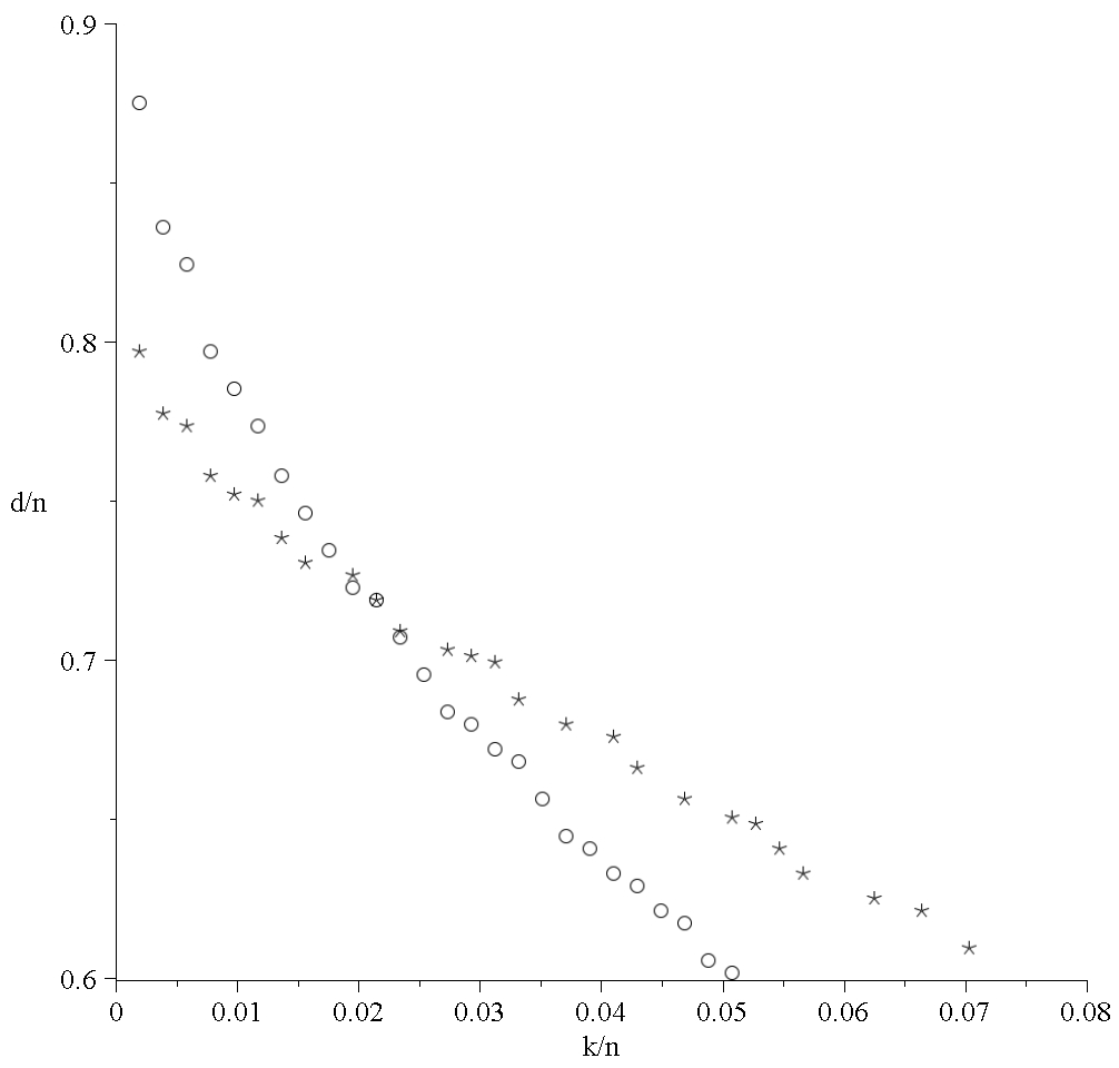
Figure 7: Improved codes from Example 10. A $\circ$ corresponds to $\widetilde{E}_{imp}(\delta)$, and an $\ast$ corresponds to $\widetilde{C}_{fim}(\delta)$.

10 Conclusion

In this paper we proposed a new bound for the minimum distance and the generalised Hamming weights of general linear code for which a generator matrix is known. We demonstrated the usefulness of our bound in the case of affine variety codes where only the first of the two order domain conditions is satisfied. For this purpose we introduced the concept of generalised $C_{ab}$ polynomials. We touched upon the connection to a bound for dual codes introduced in the recent paper [8], but leave an investigation of a possible general relation between the two bounds for further research. It is an interesting question if there exists examples where our new method improves on the Feng-Rao bound for one-point algebraic geometric codes. This would require that we do not choose $v$ as in Remark 14 and that we make extensive use of the polynomials $X_{i}^{q}-X_{i}$. Also this question is left for further research. The usual Feng-Rao bound for primary codes comes with a decoding algorithm that corrects up to half the estimated minimum distance [9]. This result holds when the bound is equipped with the well-behaving property WB. For the case of WWB or OWB no decoding algorithm is known. Finding a decoding algorithm that corrects up to half the value guaranteed by Theorem 13 would impose the missing decoding algorithms mentioned above.
Part of this research was done while the second listed author was visiting East China Normal University. We are grateful to Professor Hao Chen for his hospitality. The authors also gratefully acknowledge the support from the Danish National Research Foundation and the National Science Foundation of China (Grant No. 11061130539) for the Danish-Chinese Center for Applications of Algebraic Geometry in Coding Theory and Cryptography. The authors would like to thank Diego Ruano, Peter Beelen and Ryutaroh Matsumoto for pleasant discussions.

References

- [1] H. E. Andersen and O. Geil. Evaluation codes from order domain theory. Finite Fields Appl., 14(1):92–123, 2008.
- [2] D.A. Cox, J. Little, and D. O’Shea. Ideals, varieties, and algorithms: an introduction to computational algebraic geometry and commutative algebra, volume 10. Springer, 1997.
- [3] G. L. Feng and T. R. N. Rao. A simple approach for construction of algebraic-geometric codes from affine plane curves. IEEE Trans. Inform. Theory, 40(4):1003–1012, 1994.
- [4] J. Fitzgerald and R. F. Lax. Decoding affine variety codes using Gröbner bases. Des. Codes Cryptogr., 13(2):147–158, 1998.
- [5] O. Geil. On codes from norm-trace curves. Finite Fields Appl., 9(3):351–371, 2003.
- [6] O. Geil. Evaluation codes from an affine variety code perspective. In Edgar Martínez-Moro, Carlos Munuera, and Diego Ruano, editors, Advances in algebraic geometry codes, volume 5 of Coding Theory and Cryptology, pages 153–180. World Scientific, Singapore, 2008.
- [7] O. Geil and T. Høholdt. Footprints or generalized Bezout’s theorem. IEEE Trans. Inform. Theory, 46(2):635–641, 2000.
- [8] O. Geil and S. Martin. Further improvements on the Feng-Rao bound for dual codes. arXiv preprint arXiv:1305.1091, 2013.
- [9] O. Geil, R. Matsumoto, and D. Ruano. Feng-Rao decoding of primary codes. Finite Fields Appl., 23:35–52, 2013.
- [10] O. Geil and C. Thommesen. On the Feng-Rao bound for generalized Hamming weights. In M. P.C. Fossorier, H. Imai, S. Lin, and A. Poli, editors, Applied Algebra, Algebraic Algorithms and Error-Correcting Codes, volume 3857 of Lecture Notes in Computer Science, pages 295–306. Springer, 2006.
- [11] M. Grassl. Code Tables: Bounds on the parameters of various types of codes. http://www.codetables.de, Jun. 2013.
- [12] F. Hernando, K. Marshall, and M. E. O’Sullivan. The dimension of subcode-subfields of shortened generalized Reed–Solomon codes. Des. Codes Cryptogr., pages 1–12, 2011.
- [13] T. Høholdt, J. H. van Lint, and R. Pellikaan. Algebraic geometry codes. In Vera S. Pless and William Cary Huffman, editors, Handbook of Coding Theory, volume 1, pages 871–961. Elsevier, Amsterdam, 1998.
- [14] J. Kurihara, T. Uyematsu, and R. Matsumoto. Secret sharing schemes based on linear codes can be precisely characterized by the relative generalized Hamming weight. IEICE Trans. Fundamentals, E95-A(11):2067–2075, Nov. 2012.
- [15] Y. Luo, C. Mitrpant, A.J.H. Vinck, and K. Chen. Some new characters on the wire-tap channel of type II. IEEE Trans. Inform. Theory, 51(3):1222–1229, 2005.
- [16] R. Matsumoto. The curve. http://www.rmatsumoto.org/cab.pdf, 1998.
- [17] S. Miura. Algebraic geometric codes on certain plane curves. Electronics and Communications in Japan (Part III: Fundamental Electronic Science), 76(12):1–13, 1993.
- [18] S. Miura. Study of Error-Correcting Codes based on Algebraic Geometry. PhD thesis, Univ. Tokyo, 1997. (in Japanese).
- [19] S. Miura. Linear codes on affine algebraic curves. Trans. IEICE, J81-A(10):1398–1421, 1998.
- [20] R. Pellikaan. On the existence of order functions. Journal of Statistical Planning and Inference, 94(2):287–301, 2001.
- [21] L. Rédei. Lacunary Polynomials over Finite Fields. North-Holland Publ. Comp., Amsterdam, 1973.
- [22] G. Salazar, D. Dunn, and S. B. Graham. An improvement of the Feng-Rao bound on minimum distance. Finite Fields Appl., 12:313–335, 2006.
- [23] V. K. Wei. Generalized Hamming weights for linear codes. IEEE Trans. Inform. Theory, 37(5):1412–1418, 1991.