Analysis of the semileptonic $\Lambda_{b}\rightarrow\Lambda\ell^{+}\ell^{-}$ transition in topcolor-assisted technicolor (TC2) model

We comparatively analyze the flavor changing neutral current process of the $\Lambda_{b}\rightarrow\Lambda\ell^{+}\ell^{-}$ in the standard model as well as topcolor-assisted technicolor model using the form factors calculated via light cone QCD sum rules in full theory. In particular, we calculate the decay width, branching ratio and lepton forward-backward asymmetry related to this decay channel. We compare the results of the topcolor-assisted technicolor model with those of the standard model and debate how the results of the topcolor-assisted technicolor model depart from the standard model predictions. We also compare our results on the branching ratio and differential branching ratio with recent experimental data provided by CDF and LHCb Collaborations.

PACS number(s): 12.60.-i, 12.60.Nz, 13.30.-a, 13.30.Ce, 14.20.Mr

1 Introduction

The flavor changing neutral current (FCNC) processes in baryonic sector are promising tools in indirectly search for new physics (NP) effects besides the direct searches at large hadron colliders. Hence, both experimental and phenomenological works devoted to the analysis of these channels receive special attention nowadays. The semileptonic FCNC decay of $\Lambda_{b}\rightarrow\Lambda\ell^{+}\ell^{-}$ ($\ell=e,\mu,\tau$) is one of the most important transitions in this respect since a heavy quark with a light di-quark combination of the $\Lambda_{b}$ baryon makes this process significantly different than the B meson decays. Experimentally, the CDF Collaboration at Fermilab has firstly reported their observation of the semileptonic $\Lambda_{b}^{0}\rightarrow\Lambda\mu^{+}\mu^{-}$ decay with a statistical significance of $5.8~{}\sigma$ and $24$ signal events at $\sqrt{s}=1.96$ TeV, collected by the CDF II detector in 2011 [1]. They measured a branching ratio of $[1.73\pm 0.42(stat)\pm 0.55(syst)]\times 10^{-6}$ [1] at muon channel. Recently, the LHCb Collaboration at CERN has also reported their observation of $\Lambda_{b}^{0}\rightarrow\Lambda\mu^{+}\mu^{-}$ with a signal yield of $78\pm 12$, collected by the LHCb detector corresponding to an integrated luminosity of $1.0~{}fb^{-1}$ at $\sqrt{s}=7$ TeV [2]. They measured a branching ratio of $[0.96\pm 0.16(stat)\pm 0.13(syst)\pm 0.21(norm)]\times 10^{-6}$ at muon channel. Until now, there is no direct evidence for the NP effects beyond the standard model (SM) at present particle physics experiments. However, the ATLAS and CMS Collaborations at CERN reported their observations of a new particle like the SM Higgs boson with a mass of $\sim 125$ GeV at a statistical significance of $5~{}\sigma$ in 2012 [3, 4]. Taken into consideration the above experimental progress and recent developments at LHC, with increasing the center of mass energy, we hope we will be able to search for more FCNC decay processes as well as NP effects in near future. Therefore, theoretical calculations on NP effects to the FCNC processes using different scenarios will be required for analysis of the experimental results.

In the present work, we analyze the semileptonic FCNC channel of the $\Lambda_{b}\rightarrow\Lambda\ell^{+}\ell^{-}$ in the topcolor-assisted technicolor (TC2) model. We calculate many parameters such as decay width, branching ratio and forward-backward asymmetry (FBA) and look for the difference between the results with those of the SM predictions. We also compare our results with the above mentioned experimental data.

The technicolor (TC) mechanism provides us with an alternative explanation for the origin of masses of the electroweak gauge bosons $W^{\pm}$ and $Z^{0}$ [5]. Although the TC and extended TC (ETC) models explain the flavor symmetry and electroweak symmetry breakings (EWSB), these models are unable to answer why mass of the top quark is too large [6, 7]. In topcolor models, however, the top quark involves in a new strong interaction, spontaneously broken at some high energy scales but not confining. According to these models, the strong dynamics provide the formation of top quark condensate $\overline{t}t$ which leads to a large dynamical mass for this quark, but with unnatural fine tuning [8, 7]. Hence, a TC model containing “topcolor” scenario (TC2 model) has been developed [6]. This model explains the electroweak and flavor symmetry breakings as well as the large mass of the top quark without unnatural fine tuning. This model predicts the existence of top-pions ($\pi_{t}^{0,\pm}$), the top-Higgs ($h_{t}^{0}$) and the non-universal gauge boson ($Z^{\prime}$), which we are going to discuss the dependences of the physical quantities defining the $\Lambda_{b}\rightarrow\Lambda\ell^{+}\ell^{-}$ transition on the masses of these objects in this article. For more details of the TC2 model and some of its applications see for instance [9, 10, 11, 12] and references therein.

The outline of the article is as follows. In the next section, after briefly introducing the TC2 scenario we present the effective Hamiltonian of the transition under consideration including Wilson coefficients as well as transition amplitude and matrix elements in terms of form factors. In section 3, we calculate the differential decay width in TC2 model and numerically analyze the differential branching ratio, the branching ratio and the lepton forward-backward asymmetry and compare the obtained results with those of the SM as well as existing experimental data.

2 The semileptonic $\Lambda_{b}\rightarrow\Lambda\ell^{+}\ell^{-}$ transition in SM and the topcolor-assisted technicolor models

In this section, first we give a brief overview on TC2 model. Then we present the effective Hamiltonian in both SM and TC2 models and show how the Wilson coefficients entered to the low energy effective Hamiltonian are changed in TC2 model compare to the SM. We also present the transition matrix elements in terms of form factors in full QCD and calculate the transition amplitude of the $\Lambda_{b}\rightarrow\Lambda\ell^{+}\ell^{-}$ in both models.

2.1 The TC2 model

As we previously mentioned, the TC2 model creates an attractive scheme because it combines the TC interaction which is responsible for dynamical EWSB mechanism as an alternative to Higgs scenario as well as topcolor interaction for the third generation at scale of near $\sim 1$ TeV. This model provides an explanation of the electroweak and flavor symmetry breakings and also the large mass of top quark. This model predicts a triplet of strongly coupled pseudo-Nambu-Goldstone bosons, neutral-charged “top-pions” ($\pi_{t}^{0,\pm}$) near the top mass scale, one isospin-singlet boson, the neutral “top-Higgs” ($h_{t}^{0}$) and the non-universal gauge boson ($Z^{\prime}$). Exchange of these new particles generates flavor-changing (FC) effects which lead to changes in the Wilson coefficients compared to the SM [6].

The flavor-diagonal (FD) couplings of top-pions to the fermions are defined as [6, 7, 13, 14, 15]

$$\frac{m_{t}^{*}}{\sqrt{2}F_{\pi}}\frac{\sqrt{\nu_{w}^{2}-F_{\pi}^{2}}}{\nu_{w}}\left[i\bar{t}\gamma^{5}t\pi_{t}^{0}+\sqrt{2}\bar{t}_{R}b_{L}\pi_{t}^{+}+\sqrt{2}\bar{b}_{L}t_{R}\pi_{t}^{-}\right]$$

$$+\frac{m_{b}^{*}}{\sqrt{2}F_{\pi}}\left[i\bar{b}\gamma^{5}b\pi_{t}^{0}+\sqrt{2}\bar{t}_{L}b_{R}\pi_{t}^{+}+\sqrt{2}\bar{b}_{R}t_{L}\pi_{t}^{-}\right]+\frac{m_{l}}{\nu}\bar{l}\gamma^{5}l\pi^{0}_{t},$$ (2.1)

where $m^{*}_{t}=m_{t}(1-\varepsilon)$ and $m_{b}^{*}=m_{b}-0.1~{}\varepsilon~{}m_{t}$ denote the masses of the top and bottom quarks generated by topcolor interactions, respectively. Here, $F_{\pi}$ is the physical top-pion decay constant which is estimated from the Pagels-Stokar formula, $\nu_{w}=\nu/\sqrt{2}=174\rm~{}GeV$, wherein the $\nu$ is defined as the vacuum expectation of the Higgs field and the factor $\frac{\sqrt{\nu_{w}^{2}-F_{\pi}^{2}}}{\nu_{w}}$ represents mixing effect between the Goldstone bosons (techni-pions) and top-pions.

The FC couplings of top-pions to the quarks can be written as [16, 17, 18]

$$\frac{m_{t}^{*}}{\sqrt{2}F_{\pi}}\frac{\sqrt{\nu_{w}^{2}-F_{\pi}^{2}}}{\nu_{w}}\left[iK_{UR}^{tc}K_{UL}^{tt^{*}}\bar{t}_{L}c_{R}\pi_{t}^{0}+\sqrt{2}K_{UR}^{tc^{*}}K_{DL}^{bb}\bar{c}_{R}b_{L}\pi_{t}^{+}+\sqrt{2}K_{UR}^{tc}K_{DL}^{bb^{*}}\bar{b}_{L}c_{R}\pi_{t}^{-}\right.$$

$$\hskip 42.67912pt\left.+\sqrt{2}K_{UR}^{tc^{*}}K_{DL}^{ss}\bar{t}_{R}s_{L}\pi_{t}^{+}+\sqrt{2}K_{UR}^{tc}K_{DL}^{ss^{*}}\bar{s}_{L}t_{R}\pi_{t}^{-}\right],$$ (2.2)

where $K_{UL(R)}$ and $K_{DL(R)}$ are rotation matrices that diagonalize the up-quark and down-quark mass matrices $M_{U}$ and $M_{D}$ for the down-type left and right hand quarks, respectively. The values of the coupling parameters are given as

$$K_{UL}^{tt}\approx K_{DL}^{bb}\approx K_{DL}^{ss}\approx 1,\hskip 28.45274ptK_{UR}^{tc}\leq\sqrt{2\varepsilon-\varepsilon^{2}}.$$ (2.3)

The FD couplings of the new gauge boson $Z^{\prime}$ to the fermions are also given by [6, 7, 13, 16, 14, 15]

$${\cal L}^{FD}_{Z^{\prime}} = -\sqrt{4\pi K_{1}}\left\{Z^{\prime}_{\mu}\left[\frac{1}{2}\bar{\tau}_{L}\gamma^{\mu}\tau_{L}-\bar{\tau}_{R}\gamma^{\mu}\tau_{R}+\frac{1}{6}\bar{t}_{L}\gamma^{\mu}t_{L}+\frac{1}{6}\bar{b}_{L}\gamma^{\mu}b_{L}+\frac{2}{3}\bar{t}_{R}\gamma^{\mu}t_{R}\right.\right.$$ (2.4)

$$- \left.\left.\frac{1}{3}\bar{b}_{R}\gamma^{\mu}b_{R}\right]-\tan^{2}\theta^{\prime}Z^{\prime}_{\mu}\left[\frac{1}{6}\bar{s}_{L}\gamma^{\mu}s_{L}-\frac{1}{3}\bar{s}_{R}\gamma^{\mu}s_{R}-\frac{1}{2}\bar{\mu}_{L}\gamma^{\mu}\mu_{L}-\bar{\mu}_{R}\gamma^{\mu}\mu_{R}\right.\right.$$

$$- \left.\left.\frac{1}{2}\bar{e}_{L}\gamma^{\mu}e_{L}-\bar{e}_{R}\gamma^{\mu}e_{R}\right]\right\},$$

where $K_{1}$ is the coupling constant and it is taken in the region (0.3 - 1), $\theta^{\prime}$ is the mixing angle and $tan\theta^{\prime}=\frac{g_{1}}{\sqrt{4\pi K_{1}}}$ with $g_{1}$ being the ordinary hypercharge gauge coupling constant.

The FC couplings of the non-universal $Z^{\prime}$ gauge boson to the fermions can be written as [19]

$${\cal L}^{FC}_{Z^{\prime}}=-\frac{g_{1}}{2}\cot{\theta^{\prime}}Z^{\prime\mu}\left\{\frac{1}{3}D_{L}^{bb}D_{L}^{bs*}\bar{s}_{L}\gamma_{\mu}b_{L}-\frac{2}{3}D_{R}^{bb}D_{R}^{bs*}\bar{s}_{R}\gamma_{\mu}b_{R}+{\rm h.c.}\right\},$$ (2.5)

where $D_{L}$ and $D_{R}$ are matrices rotate the weak eigen-basis to the mass ones for down-type left and right hand quarks, respectively.

2.2 The effective Hamiltonian and Wilson Coefficients

The $\Lambda_{b}\rightarrow\Lambda\ell^{+}\ell^{-}$ decay is governed by $b\rightarrow s\ell^{+}\ell^{-}$ transition at quark level in SM, whose effective Hamiltonian is given by [20, 21, 22, 23]

$${\cal H}^{eff}_{SM} = \frac{G_{F}\alpha_{em}V_{tb}V_{ts}^{\ast}}{2\sqrt{2}\pi}\Bigg{[}C^{eff}_{9}\bar{s}\gamma_{\mu}(1-\gamma_{5})b\,\bar{\ell}\gamma^{\mu}\ell+C_{10}\bar{s}\gamma_{\mu}(1-\gamma_{5})b\,\bar{\ell}\gamma^{\mu}\gamma_{5}\ell$$ (2.6)

$$- 2m_{b}C^{eff}_{7}\frac{1}{q^{2}}\bar{s}i\sigma_{\mu\nu}q^{\nu}(1+\gamma_{5})b\,\bar{\ell}\gamma^{\mu}\ell\Bigg{]}~{},$$

where $G_{F}$ is the Fermi coupling constant, $\alpha_{em}$ is the fine structure constant, $V_{tb}$ and $V_{ts}^{\ast}$ are elements of the Cabibbo-Kobayashi-Maskawa (CKM) matrix, $q^{2}$ is the transferred momentum squared and the $C^{eff}_{7}$, $C^{eff}_{9}$, $C_{10}$ are the Wilson coefficients. Our main task in the following are to present the expressions of the Wilson coefficients. The Wilson coefficient $C_{7}^{eff}$ in leading log approximation in SM is given by [24, 25, 26, 27]

$$C_{7}^{eff}(\mu_{b})\!\!\! = \!\!\!\eta^{\frac{16}{23}}C_{7}(\mu_{W})+\frac{8}{3}\left(\eta^{\frac{14}{23}}-\eta^{\frac{16}{23}}\right)C_{8}(\mu_{W})+C_{2}(\mu_{W})\sum_{i=1}^{8}h_{i}\eta^{a_{i}}~{},$$

where

$$\eta\!\!\! = \!\!\!\frac{\alpha_{s}(\mu_{W})}{\alpha_{s}(\mu_{b})}~{},$$ (2.8)

and

$$\alpha_{s}(x)=\frac{\alpha_{s}(m_{Z})}{1-\beta_{0}\frac{\alpha_{s}(m_{Z})}{2\pi}\ln(\frac{m_{Z}}{x})}~{},$$ (2.9)

with $\alpha_{s}(m_{Z})=0.118$ and $\beta_{0}=\frac{23}{3}$. The remaining functions in Eq.(2.2) are written as

$$C_{7}(\mu_{W})=-\frac{1}{2}D^{\prime~{}SM}_{0}(x_{t})~{},~{}~{}C_{8}(\mu_{W})=-\frac{1}{2}E^{\prime~{}SM}_{0}(x_{t})~{},~{}~{}C_{2}(\mu_{W})=1~{},$$ (2.10)

where the functions $D^{\prime~{}SM}_{0}(x_{t})$ and $E^{\prime~{}SM}_{0}(x_{t})$ with $x_{t}=\frac{m_{t}^{2}}{m_{W}^{2}}$ are given by

$$D^{\prime~{}SM}_{0}(x_{t})\!\!\! = \!\!\!-\frac{(8x_{t}^{3}+5x_{t}^{2}-7x_{t})}{12(1-x_{t})^{3}}+\frac{x_{t}^{2}(2-3x_{t})}{2(1-x_{t})^{4}}\ln x_{t}~{},$$ (2.11)

and

$$E^{\prime~{}SM}_{0}(x_{t})\!\!\! = \!\!\!-\frac{x_{t}(x_{t}^{2}-5x_{t}-2)}{4(1-x_{t})^{3}}+\frac{3x_{t}^{2}}{2(1-x_{t})^{4}}\ln x_{t}~{}.$$ (2.12)

The coefficients $h_{i}$ and $a_{i}$ in Eq.(2.2), with i running from 1 to 8, are also given by [25, 26]

$$\frac{}{}\begin{array}[]{rrrrrrrrrl}h_{i}=(\!\!&2.2996,&-1.0880,&-\frac{3}{7},&-\frac{1}{14},&-0.6494,&-0.0380,&-0.0186,&-0.0057&\!\!)\vspace{0.1cm},\\ \end{array}$$ (2.13)

and

$$\frac{}{}\begin{array}[]{rrrrrrrrrl}a_{i}=(\!\!&\frac{14}{23},&\frac{16}{23},&\frac{6}{23},&-\frac{12}{23},&0.4086,&-0.4230,&-0.8994,&0.1456&\!\!).\end{array}$$ (2.14)

The Wilson coefficient $C_{9}^{eff}$ in SM is expressed as [25, 26]

$$C_{9}^{eff}(\hat{s}^{\prime}) = C_{9}^{NDR}\eta(\hat{s}^{\prime})+h(z,\hat{s}^{\prime})\left(3C_{1}+C_{2}+3C_{3}+C_{4}+3C_{5}+C_{6}\right)$$ (2.15)

$$-\frac{1}{2}h(1,\hat{s}^{\prime})\left(4C_{3}+4C_{4}+3C_{5}+C_{6}\right)$$

$$-\frac{1}{2}h(0,\hat{s}^{\prime})\left(C_{3}+3C_{4}\right)+\frac{2}{9}\left(3C_{3}+C_{4}+3C_{5}+C_{6}\right),$$

where $\hat{s}^{\prime}=\frac{q^{2}}{m_{b}^{2}}$ with $q^{2}$ lies in the interval $4m_{l}^{2}\leq q^{2}\leq(m_{\Lambda_{b}}-m_{\Lambda})^{2}$. The $C_{9}^{NDR}$ in the naive dimensional regularization (NDR) scheme is given as

$$C_{9}^{NDR} = P_{0}^{NDR}+\frac{Y^{SM}}{\sin^{2}\theta_{W}}-4Z^{SM}+P_{E}E^{SM},$$ (2.16)

where $P_{0}^{NDR}=2.60\pm 0.25$, $\sin^{2}\theta_{W}=0.23$, $Y^{SM}=0.98$ and $Z^{SM}=0.679$ [25, 26, 27]. The last term in Eq.(2.16) is ignored due to smallness of the value of $P_{E}$. The $\eta(\hat{s}^{\prime})$ in Eq.(2.15) is also defined as

$$\eta(\hat{s}^{\prime}) = 1+\frac{\alpha_{s}(\mu_{b})}{\pi}\,\omega(\hat{s}^{\prime}),$$ (2.17)

with

$$\omega(\hat{s}^{\prime}) = -\frac{2}{9}\pi^{2}-\frac{4}{3}\mbox{Li}_{2}(\hat{s}^{\prime})-\frac{2}{3}\ln\hat{s}^{\prime}\ln(1-\hat{s}^{\prime})-\frac{5+4\hat{s}^{\prime}}{3(1+2\hat{s}^{\prime})}\ln(1-\hat{s}^{\prime})-$$ (2.18)

$$\frac{2\hat{s}^{\prime}(1+\hat{s}^{\prime})(1-2\hat{s}^{\prime})}{3(1-\hat{s}^{\prime})^{2}(1+2\hat{s}^{\prime})}\ln\hat{s}^{\prime}+\frac{5+9\hat{s}^{\prime}-6\hat{s}^{\prime 2}}{6(1-\hat{s}^{\prime})(1+2\hat{s}^{\prime})}.$$

The function $h(y,\hat{s}^{\prime})$ is given as

$$h(y,\hat{s}^{\prime}) = -\frac{8}{9}\ln\frac{m_{b}}{\mu_{b}}-\frac{8}{9}\ln y+\frac{8}{27}+\frac{4}{9}x$$ (2.21)

$$-\frac{2}{9}(2+x)|1-x|^{1/2}\left\{\begin{array}[]{ll}\left(\ln\left|\frac{\sqrt{1-x}+1}{\sqrt{1-x}-1}\right|-i\pi\right),&\mbox{for }x\equiv\frac{4z^{2}}{\hat{s}^{\prime}}<1\\ 2\arctan\frac{1}{\sqrt{x-1}},&\mbox{for }x\equiv\frac{4z^{2}}{\hat{s}^{\prime}}>1,\end{array}\right.$$

where $y=1$ or $y=z=\frac{m_{c}}{m_{b}}$ and

$$h(0,\hat{s}^{\prime}) = \frac{8}{27}-\frac{8}{9}\ln\frac{m_{b}}{\mu_{b}}-\frac{4}{9}\ln\hat{s}^{\prime}+\frac{4}{9}i\pi.$$ (2.23)

At $\mu_{b}=5~{}GeV$ scale, the coefficients $C_{j}$ (j=1,…6) are given by [27]

$$C_{j}=\sum_{i=1}^{8}k_{ji}\eta^{a_{i}}\qquad(j=1,...6)\vspace{0.2cm},$$ (2.24)

where the constants $k_{ji}$ are given as

$$\frac{}{}\begin{array}[]{rrrrrrrrrl}k_{1i}=(\!\!&0,&0,&\frac{1}{2},&-\frac{1}{2},&0,&0,&0,&0&\!\!),\vspace{0.1cm}\\ k_{2i}=(\!\!&0,&0,&\frac{1}{2},&\frac{1}{2},&0,&0,&0,&0&\!\!),\vspace{0.1cm}\\ k_{3i}=(\!\!&0,&0,&-\frac{1}{14},&\frac{1}{6},&0.0510,&-0.1403,&-0.0113,&0.0054&\!\!),\vspace{0.1cm}\\ k_{4i}=(\!\!&0,&0,&-\frac{1}{14},&-\frac{1}{6},&0.0984,&0.1214,&0.0156,&0.0026&\!\!),\vspace{0.1cm}\\ k_{5i}=(\!\!&0,&0,&0,&0,&-0.0397,&0.0117,&-0.0025,&0.0304&\!\!),\vspace{0.1cm}\\ k_{6i}=(\!\!&0,&0,&0,&0,&0.0335,&0.0239,&-0.0462,&-0.0112&\!\!).\vspace{0.1cm}\\ \end{array}$$ (2.25)

The Wilson coefficient $C_{10}$ in SM is scale-independent and has the following explicit expression:

$$C_{10}=-\frac{Y^{SM}}{\sin^{2}\theta_{W}}~{}.$$ (2.26)

The effective Hamiltonian for $b\rightarrow s\ell^{+}\ell^{-}$ transition in TC2 model is given by [12]

$${\cal H}^{eff}_{TC2} = \frac{G_{F}\alpha_{em}V_{tb}V_{ts}^{\ast}}{2\sqrt{2}\pi}\Bigg{[}\widetilde{C}^{eff}_{9}\bar{s}\gamma_{\mu}(1-\gamma_{5})b\,\bar{\ell}\gamma^{\mu}\ell+\widetilde{C}_{10}\bar{s}\gamma_{\mu}(1-\gamma_{5})b\,\bar{\ell}\gamma^{\mu}\gamma_{5}\ell$$ (2.27)

$$- 2m_{b}\widetilde{C}^{eff}_{7}\frac{1}{q^{2}}\bar{s}i\sigma_{\mu\nu}q^{\nu}(1+\gamma_{5})b\,\bar{\ell}\gamma^{\mu}\ell+C_{Q_{1}}\bar{s}(1+\gamma_{5})b\bar{\ell}\ell$$

$$+ C_{Q_{2}}\bar{s}(1+\gamma_{5})b\bar{\ell}\gamma_{5}\ell\Bigg{]}~{},$$

where $\widetilde{C}^{eff}_{7}$, $\widetilde{C}^{eff}_{9}$, $\widetilde{C}_{10}$, $C_{Q_{1}}$ and $C_{Q_{2}}$ are new Wilson coefficients. The $\widetilde{C}^{eff}_{7}$, $\widetilde{C}^{eff}_{9}$ and $\widetilde{C}_{10}$ contain contributions from both the SM and TC2 models. The charged top-pions $\pi_{t}^{\pm}$ only give contributions to the Wilson coefficient $\widetilde{C}^{eff}_{7}$ while the non-universal gauge boson $Z^{\prime}$ contributes to the Wilson coefficients $\widetilde{C}^{eff}_{9}$ and $\widetilde{C}_{10}$. In the following, we present the explicit expressions of the Wilson coefficients $C_{7}(\mu_{W})$ and $C_{8}(\mu_{W})$ entered to Eq.(2.2) in TC2 model. The new photonic-and gluonic-penguin diagrams in TC2 model can be gotten by replacement of the internal $W^{\pm}$ lines in SM penguin diagrams with unit-charged scalar ($\pi_{1}^{\pm}$, $\pi_{8}^{\pm}$ and $\pi_{t}^{\pm}$) lines (for more information, see Ref. [9]). As a result, the Wilson coefficients $\widetilde{C}_{7}(\mu_{W})$ and $\widetilde{C}_{8}(\mu_{W})$ in TC2 take the following forms [12, 28]:

$$\widetilde{C}_{7}(\mu_{W})=-\frac{1}{2}D^{\prime~{}TC2tot}_{0}(x_{t},z_{t})~{},~{}~{}\widetilde{C}_{8}(\mu_{W})=-\frac{1}{2}E^{\prime~{}TC2tot}_{0}(x_{t},z_{t})~{},$$ (2.28)

where

$$D^{\prime~{}TC2tot}_{0}(x_{t},z_{t}) = D_{0}^{\prime~{}SM}(x_{t})+D_{0}^{\prime~{}TC2}(z_{t}),$$

$$E^{\prime~{}TC2tot}_{0}(x_{t},z_{t}) = E_{0}^{\prime~{}SM}(x_{t})+E_{0}^{\prime~{}TC2}(z_{t}),$$ (2.29)

and

$$D_{0}^{\prime~{}TC2}(z_{t}) = \frac{1}{8\sqrt{2}G_{F}F_{\pi}^{2}}\left[-\frac{22-53z_{t}+25z_{t}^{2}}{18(1-z_{t})^{3}}-\frac{3z_{t}-8z_{t}^{2}+4z_{t}^{3}}{3(1-z_{t})^{4}}{\rm log}[z_{t}]\right],$$

$$E_{0}^{\prime~{}TC2}(z_{t}) = \frac{1}{8\sqrt{2}G_{F}F_{\pi}^{2}}\left[-\frac{5-19z_{t}+20z_{t}^{2}}{6(1-z_{t})^{3}}+\frac{z_{t}^{2}-2z_{t}^{3}}{(1-z_{t})^{4}}{\rm log}[z_{t}]\right],$$ (2.30)

with $z_{t}={m^{*}_{t}}^{2}/m_{\pi_{t}^{\pm}}^{2}$.
There are new contributions coming from the non-universal gauge boson $Z^{\prime}$ in TC2 model to the $Y^{SM}$ and $Z^{SM}$ entered to the ${C}_{9}^{NDR}$ in Eq.(2.15) [12]. The $\widetilde{C}_{9}^{NDR}$ in TC2 model is given by

$$\widetilde{C}_{9}^{NDR}=P_{0}^{NDR}+\frac{Y^{TC2tot}(y_{t})}{\sin^{2}\theta_{W}}-4Z^{TC2tot}(y_{t}),$$ (2.31)

where

$$Y^{TC2tot}(y_{t}) = Y^{SM}+Y^{TC2}(y_{t}),$$

$$Z^{TC2tot}(y_{t}) = Z^{SM}+Z^{TC2}(y_{t}).$$ (2.32)

The functions $Y^{TC2}(y_{t})$ and $Z^{TC2}(y_{t})$ are given by the following expressions in the case of $e$ or $\mu$ in the final state [11, 12]:

$$Y^{TC2}(y_{t})=Z^{TC2}(y_{t}) = \frac{-tan^{2}\theta^{\prime}M_{Z}^{2}}{M_{Z^{\prime}}^{2}}\Big{[}K_{ab}(y_{t})+K_{c}(y_{t})+K_{d}(y_{t})\Big{]},$$ (2.33)

with $y_{t}=m_{t}^{*2}/m_{W}^{2}$. In the case of $\tau$ as final leptonic state, the factor $-tan^{2}\theta^{\prime}$ in the above equation is replaced by 1. The functions in Eq.(2.33) are also defined as [29]

$$K_{ab}(y_{t}) = \frac{8}{3}(tan^{2}\theta^{\prime}-1)\frac{F_{1}(y_{t})}{(v_{d}+a_{d})},$$

$$K_{c}(y_{t}) = \frac{16F_{2}(y_{t})}{3(v_{u}-a_{u})}-\frac{8F_{3}(y_{t})}{3(v_{u}+a_{u})},$$

$$K_{d}(y_{t}) = \frac{16F_{4}(y_{t})}{3(v_{u}-a_{u})}+\frac{8F_{5}(y_{t})}{3(v_{u}+a_{u})},$$ (2.34)

where

$$F_{1}(y_{t}) = -\Big{[}0.5(Q-1)\sin^{2}\theta_{W}+0.25\Big{]}\Bigg{\{}y_{t}^{2}ln(y_{t})/(y_{t}-1)^{2}-y_{t}/(y_{t}-1)$$

$$- y_{t}\Big{[}0.5\Big{(}-0.5772+ln(4\pi)-ln(M_{W}^{2})\Big{)}+0.75-0.5\Big{(}x^{2}ln(y_{t})/(y_{t}-1)^{2}-1/(y_{t}-1)\Big{)}\Big{]}\Bigg{\}}$$

$$\Big{[}(1+y_{t})/(y_{t}-2)\Big{]},$$

$$F_{2}(y_{t}) = \Big{(}0.5Q\sin^{2}\theta_{W}-0.25\Big{)}\Big{[}y_{t}^{2}ln(y_{t})/(y_{t}-1)^{2}-2y_{t}ln(y_{t})/(y_{t}-1)^{2}+y_{t}/(y_{t}-1)\Big{]},$$

$$F_{3}(y_{t}) = -Q\sin^{2}\theta_{W}\Big{[}y_{t}/(y_{t}-1)-y_{t}ln(y_{t})/(y_{t}-1)^{2}\Big{]},$$

$$F_{4}(y_{t}) = 0.25\Big{(}4\sin^{2}\theta_{W}/3-1\Big{)}\Big{[}y_{t}^{2}ln(y_{t})/(y_{t}-1)^{2}-y_{t}-y_{t}/(y_{t}-1)\Big{]},$$

$$F_{5}(y_{t}) = -0.25Q\sin^{2}\theta_{W}y_{t}\Big{[}-0.5772+ln(4\pi)-ln(M_{W}^{2})+1-y_{t}ln(y_{t})/(y_{t}-1)\Big{]}$$ (2.35)

$$- \sin^{2}\theta_{W}/6\Big{[}y_{t}^{2}ln(y_{t})/(y_{t}-1)^{2}-y_{t}-y_{t}/(y_{t}-1)\Big{]},$$

and $a_{u,d}=I_{3}$, $v_{u,d}=I_{3}-2Q_{u,d}\sin^{2}\theta_{W}$ with $u$ and $d$ representing the up and down type quarks, respectively.
The Wilson coefficients $C_{Q_{1}}$ and $C_{Q_{2}}$ appeared in the effective Hamiltonian in TC2 model belong to the neutral top-pion $\pi_{t}^{0}$ and top-Higgs $h_{t}^{0}$ contributing to the rare decays. The coefficient $C_{Q_{1}}$ in TC2 model is given by [11]

$$C_{Q_{1}}=\frac{\sqrt{\nu_{w}^{2}-F_{\pi}^{2}}}{\nu_{w}}\left(\frac{m_{b}^{*}m_{l}\nu}{2\sqrt{2}sin^{2}\theta_{w}F_{\pi}m_{h_{t}^{0}}^{2}}C_{0}(x_{t})+\frac{V_{ts}m_{l}m_{t}m_{b}^{*2}M_{W}^{2}}{4\sqrt{2}g_{2}^{4}F_{\pi}^{2}m_{h_{t}^{0}}^{2}}C(x_{s})\right),$$ (2.36)

where the Inami-Lim function $C_{0}(x_{t})$ is defined by [27]

$$C_{0}(x_{t}) = \frac{x_{t}}{8}\left[\frac{x_{t}-6}{x_{t}-1}+\frac{3x_{t}+2}{(x_{t}-1)^{2}}\ln x_{t}\right].$$ (2.37)

The $C(x_{s})$ function in Eq.(2.36) is also given as [12]

$$C(x_{s}) = \frac{F_{6}(x)}{-[0.5(Q-1)\sin^{2}\theta_{W}+0.25]},$$ (2.38)

with

$$F_{6}(x_{s}) = -\Big{[}0.5(Q-1)\sin^{2}\theta_{W}+0.25\Big{]}\Bigg{\{}x_{s}^{2}ln(x_{s})/(x_{s}-1)^{2}-x_{s}/(x_{s}-1)$$ (2.39)

$$- x_{s}\Big{[}0.5\Big{(}-0.5772+ln(4\pi)-ln(M_{W}^{2})\Big{)}+0.75-0.5\Big{(}x^{2}ln(x_{s})/(x_{s}-1)^{2}$$

$$- 1/(x_{s}-1)\Big{)}\Big{]}\Bigg{\}},$$

where $x_{s}={m^{*}_{t}}^{2}/m_{\pi_{t}^{0}}^{2}$ and the $g_{2}$ is the $SU(2)$ coupling constant. Since, the neutral top-Higgs coupling with fermions differ from that of neutral top-pion by a factor of $\gamma_{5}$, the form of $C_{Q_{2}}$ is the same as $C_{Q_{1}}$ except for the masses of the scalar particles [11].

2.3 Transition amplitude and matrix elements

The transition amplitude for $\Lambda_{b}\rightarrow\Lambda\ell^{+}\ell^{-}$ decay is obtained by sandwiching the effective Hamiltonian between the initial and final baryonic states

$${\cal M}^{\Lambda_{b}\rightarrow\Lambda\ell^{+}\ell^{-}}=\langle\Lambda(p_{\Lambda})\mid{\cal H}^{eff}\mid\Lambda_{b}(p_{\Lambda_{b}})\rangle,$$ (2.40)

where $p_{\Lambda_{b}}$ and $p_{\Lambda}$ are momenta of the $\Lambda_{b}$ and $\Lambda$ baryons, respectively. In order to calculate the transition amplitude, we need to define the following matrix elements in terms of twelve form factors in full QCD:

$$\langle\Lambda(p_{\Lambda})\mid\bar{s}\gamma_{\mu}(1-\gamma_{5})b\mid\Lambda_{b}(p_{\Lambda_{b}})\rangle\!\!\! = \!\!\!\bar{u}_{\Lambda}(p_{\Lambda})\Bigg{[}\gamma_{\mu}f_{1}(q^{2})+{i}\sigma_{\mu\nu}q^{\nu}f_{2}(q^{2})+q^{\mu}f_{3}(q^{2})$$

$$- \!\!\!\gamma_{\mu}\gamma_{5}g_{1}(q^{2})-{i}\sigma_{\mu\nu}\gamma_{5}q^{\nu}g_{2}(q^{2})-q^{\mu}\gamma_{5}g_{3}(q^{2})\vphantom{\int_{0}^{x_{2}}}\Bigg{]}u_{\Lambda_{b}}(p_{\Lambda_{b}})~{},$$

$$\langle\Lambda(p_{\Lambda})\mid\bar{s}i\sigma_{\mu\nu}q^{\nu}(1+\gamma_{5})b\mid\Lambda_{b}(p_{\Lambda_{b}})\rangle\!\!\! = \!\!\!\bar{u}_{\Lambda}(p_{\Lambda})\Bigg{[}\gamma_{\mu}f_{1}^{T}(q^{2})+{i}\sigma_{\mu\nu}q^{\nu}f_{2}^{T}(q^{2})+q^{\mu}f_{3}^{T}(q^{2})$$

$$+ \!\!\!\gamma_{\mu}\gamma_{5}g_{1}^{T}(q^{2})+{i}\sigma_{\mu\nu}\gamma_{5}q^{\nu}g_{2}^{T}(q^{2})+q^{\mu}\gamma_{5}g_{3}^{T}(q^{2})\vphantom{\int_{0}^{x_{2}}}\Bigg{]}u_{\Lambda_{b}}(p_{\Lambda_{b}})~{},$$

and

$$\langle\Lambda(p_{\Lambda})\mid\bar{s}(1+\gamma_{5})b\mid\Lambda_{b}(p_{\Lambda_{b}})\rangle\!\!\! = \!\!\!\frac{1}{m_{b}}\bar{u}_{\Lambda}(p_{\Lambda})\Bigg{[}{\not\!q}f_{1}(q^{2})+{i}q^{\mu}\sigma_{\mu\nu}q^{\nu}f_{2}(q^{2})+q^{2}f_{3}(q^{2})$$

$$- \!\!\!{\not\!q}\gamma_{5}g_{1}(q^{2})-{i}q^{\mu}\sigma_{\mu\nu}\gamma_{5}q^{\nu}g_{2}(q^{2})-q^{2}\gamma_{5}g_{3}(q^{2})\vphantom{\int_{0}^{x_{2}}}\Bigg{]}u_{\Lambda_{b}}(p_{\Lambda_{b}})~{},$$

where the $u_{\Lambda_{b}}$ and $u_{\Lambda}$ are spinors of the initial and final baryons. By the way, the $f^{(T)}_{i}$ and $g^{(T)}_{i}$ with $i=1,2$ and $3$ are transition form factors.

Using the above transition matrix elements, we find the transition amplitude for $\Lambda_{b}\rightarrow\Lambda\ell^{+}\ell^{-}$ in TC2 model as

$${\cal M}_{TC2}^{\Lambda_{b}\rightarrow\Lambda\ell^{+}\ell^{-}}=\frac{G_{F}\alpha_{em}V_{tb}V_{ts}^{\ast}}{2\sqrt{2}\pi}\Bigg{\{}$$

$$\Big{[}{\bar{u}}_{\Lambda}({p}_{\Lambda})(\gamma_{\mu}[{\cal A}_{1}R+{\cal B}_{1}L]+{i}\sigma_{\mu\nu}q^{\nu}[{\cal A}_{2}R+{\cal B}_{2}L]+q^{\mu}[{\cal A}_{3}R+{\cal B}_{3}L])u_{\Lambda_{b}}(p_{\Lambda_{b}})\Big{]}\,(\bar{\ell}\gamma^{\mu}\ell)$$

$$+ \Big{[}{\bar{u}}_{\Lambda}({p}_{\Lambda})(\gamma_{\mu}[{\cal D}_{1}R+{\cal E}_{1}L]+{i}\sigma_{\mu\nu}q^{\nu}[{\cal D}_{2}R+{\cal E}_{2}L]+q^{\mu}[{\cal D}_{3}R+{\cal E}_{3}L])u_{\Lambda_{b}}(p_{\Lambda_{b}})\Big{]}\,(\bar{\ell}\gamma^{\mu}\gamma_{5}\ell)$$

$$+ \Big{[}{\bar{u}}_{\Lambda}({p}_{\Lambda})({\not\!q}[{\cal G}_{1}R+{\cal H}_{1}L]+{i}q^{\mu}\sigma_{\mu\nu}q^{\nu}[{\cal G}_{2}R+{\cal H}_{2}L]+q^{2}[{\cal G}_{3}R+{\cal H}_{3}L])u_{\Lambda_{b}}(p_{\Lambda_{b}})\Big{]}\,(\bar{\ell}\ell)$$

$$+ \Big{[}{\bar{u}}_{\Lambda}({p}_{\Lambda})({\not\!q}[{\cal K}_{1}R+{\cal S}_{1}L]+{i}q^{\mu}\sigma_{\mu\nu}q^{\nu}[{\cal K}_{2}R+{\cal S}_{2}L]+q^{2}[{\cal K}_{3}R+{\cal S}_{3}L])u_{\Lambda_{b}}(p_{\Lambda_{b}})\Big{]}\,(\bar{\ell}\gamma_{5}\ell)\Bigg{\}}~{},$$

where $R=(1+\gamma_{5})/2$ and $L=(1-\gamma_{5})/2$. The calligraphic coefficients are defined as

$${\cal A}_{1}\!\!\! = \!\!\!(f_{1}-g_{1})~{}\widetilde{C}_{9}^{eff}~{}-~{}2m_{b}\frac{1}{q^{2}}~{}(f_{1}^{T}+g_{1}^{T})~{}\widetilde{C}_{7}^{eff}~{},~{}~{}~{}~{}~{}~{}~{}~{}~{}~{}{\cal G}_{1}=\frac{1}{m_{b}}~{}(f_{1}-g_{1})~{}C_{Q_{1}}~{},~{}$$

$${\cal A}_{2}={\cal A}_{1}(1\rightarrow 2)~{},~{}~{}~{}~{}~{}~{}~{}~{}~{}~{}~{}~{}~{}~{}~{}~{}~{}~{}~{}~{}~{}~{}~{}~{}~{}~{}~{}~{}~{}~{}~{}~{}~{}~{}~{}~{}~{}~{}~{}~{}~{}~{}~{}~{}~{}~{}~{}~{}~{}~{}{\cal G}_{2}={\cal G}_{1}\left(1\rightarrow 2\right)~{},~{}~{}~{}~{}$$

$${\cal A}_{3}={\cal A}_{1}\left(1\rightarrow 3\right)~{},~{}~{}~{}~{}~{}~{}~{}~{}~{}~{}~{}~{}~{}~{}~{}~{}~{}~{}~{}~{}~{}~{}~{}~{}~{}~{}~{}~{}~{}~{}~{}~{}~{}~{}~{}~{}~{}~{}~{}~{}~{}~{}~{}~{}~{}~{}~{}~{}~{}~{}{\cal G}_{3}={\cal G}_{1}\left(1\rightarrow 3\right)~{},~{}~{}~{}~{}$$

$${\cal B}_{1}\!\!\! = \!\!\!{\cal A}_{1}(g_{1}\rightarrow-g_{1}~{};~{}g_{1}^{T}\rightarrow-g_{1}^{T})~{},~{}~{}~{}~{}~{}~{}~{}~{}~{}~{}~{}~{}~{}~{}~{}~{}~{}~{}~{}~{}~{}~{}~{}~{}~{}~{}~{}~{}~{}{\cal H}_{1}={\cal G}_{1}(g_{1}\rightarrow-g_{1})~{},~{}~{}~{}~{}~{}$$

$${\cal B}_{2}={\cal B}_{1}\left(1\rightarrow 2\right)~{},~{}~{}~{}~{}~{}~{}~{}~{}~{}~{}~{}~{}~{}~{}~{}~{}~{}~{}~{}~{}~{}~{}~{}~{}~{}~{}~{}~{}~{}~{}~{}~{}~{}~{}~{}~{}~{}~{}~{}~{}~{}~{}~{}~{}~{}~{}~{}~{}~{}~{}{\cal H}_{2}={\cal H}_{1}\left(1\rightarrow 2\right)~{},~{}~{}~{}$$

$${\cal B}_{3}={\cal B}_{1}\left(1\rightarrow 3\right)~{},~{}~{}~{}~{}~{}~{}~{}~{}~{}~{}~{}~{}~{}~{}~{}~{}~{}~{}~{}~{}~{}~{}~{}~{}~{}~{}~{}~{}~{}~{}~{}~{}~{}~{}~{}~{}~{}~{}~{}~{}~{}~{}~{}~{}~{}~{}~{}~{}~{}~{}{\cal H}_{3}={\cal H}_{1}\left(1\rightarrow 3\right)~{},~{}~{}~{}$$

$${\cal D}_{1}\!\!\! = \!\!\!(f_{1}-g_{1})~{}\widetilde{C}_{10}~{},~{}~{}~{}~{}~{}~{}~{}~{}~{}~{}~{}~{}~{}~{}~{}~{}~{}~{}~{}~{}~{}~{}~{}~{}~{}~{}~{}~{}~{}~{}~{}~{}~{}~{}~{}~{}~{}~{}~{}~{}~{}~{}~{}~{}~{}~{}~{}{\cal K}_{1}=\frac{1}{m_{b}}~{}(f_{1}-g_{1})~{}C_{Q_{2}}~{},~{}$$

$${\cal D}_{2}={\cal D}_{1}\left(1\rightarrow 2\right)~{},~{}~{}~{}~{}~{}~{}~{}~{}~{}~{}~{}~{}~{}~{}~{}~{}~{}~{}~{}~{}~{}~{}~{}~{}~{}~{}~{}~{}~{}~{}~{}~{}~{}~{}~{}~{}~{}~{}~{}~{}~{}~{}~{}~{}~{}~{}~{}~{}~{}~{}{\cal K}_{2}={\cal K}_{1}\left(1\rightarrow 2\right)~{},~{}~{}~{}~{}$$

$${\cal D}_{3}={\cal D}_{1}\left(1\rightarrow 3\right)~{},~{}~{}~{}~{}~{}~{}~{}~{}~{}~{}~{}~{}~{}~{}~{}~{}~{}~{}~{}~{}~{}~{}~{}~{}~{}~{}~{}~{}~{}~{}~{}~{}~{}~{}~{}~{}~{}~{}~{}~{}~{}~{}~{}~{}~{}~{}~{}~{}~{}~{}{\cal K}_{3}={\cal K}_{1}\left(1\rightarrow 3\right)~{},~{}~{}~{}~{}~{}$$

$${\cal E}_{1}={\cal D}_{1}(g_{1}\rightarrow-g_{1})~{},~{}~{}~{}~{}~{}~{}~{}~{}~{}~{}~{}~{}~{}~{}~{}~{}~{}~{}~{}~{}~{}~{}~{}~{}~{}~{}~{}~{}~{}~{}~{}~{}~{}~{}~{}~{}~{}~{}~{}~{}~{}~{}~{}~{}~{}~{}~{}{\cal S}_{1}={\cal K}_{1}(g_{1}\rightarrow-g_{1})~{},~{}$$

$${\cal E}_{2}={\cal E}_{1}\left(1\rightarrow 2\right)~{},~{}~{}~{}~{}~{}~{}~{}~{}~{}~{}~{}~{}~{}~{}~{}~{}~{}~{}~{}~{}~{}~{}~{}~{}~{}~{}~{}~{}~{}~{}~{}~{}~{}~{}~{}~{}~{}~{}~{}~{}~{}~{}~{}~{}~{}~{}~{}~{}~{}~{}~{}~{}{\cal S}_{2}={\cal S}_{1}\left(1\rightarrow 2\right)~{},~{}~{}~{}~{}~{}$$

$${\cal E}_{3}={\cal E}_{1}\left(1\rightarrow 3\right)~{},~{}~{}~{}~{}~{}~{}~{}~{}~{}~{}~{}~{}~{}~{}~{}~{}~{}~{}~{}~{}~{}~{}~{}~{}~{}~{}~{}~{}~{}~{}~{}~{}~{}~{}~{}~{}~{}~{}~{}~{}~{}~{}~{}~{}~{}~{}~{}~{}~{}~{}~{}~{}{\cal S}_{3}={\cal S}_{1}\left(1\rightarrow 3\right)~{}.~{}~{}~{}~{}~{}$$

3 Physical Observables

In this section, we calculate some physical observables such as differential decay width, differential branching ratio, branching ratio and the lepton forward-backward asymmetry for the decay channel under consideration.

3.1 The differential decay width

In the present subsection, using the above-mentioned amplitude, we find the differential decay rate in terms of form factors in full theory in TC2 model as

$$\frac{d^{2}\Gamma}{d\hat{s}dz}(z,\hat{s})=\frac{G_{F}^{2}\alpha^{2}_{em}m_{\Lambda_{b}}}{16384\pi^{5}}|V_{tb}V_{ts}^{*}|^{2}v\sqrt{\lambda(1,r,\hat{s})}\,\Bigg{[}{\cal T}_{0}(\hat{s})+{\cal T}_{1}(\hat{s})z+{\cal T}_{2}(\hat{s})z^{2}\Bigg{]}~{},$$

(3.46)

where $v=\sqrt{1-\frac{4m_{\ell}^{2}}{q^{2}}}$ is the lepton velocity, $\lambda=\lambda(1,r,\hat{s})=(1-r-\hat{s})^{2}-4r\hat{s}$ is the usual triangle function with $\hat{s}=q^{2}/m^{2}_{\Lambda_{b}}$, $r=m^{2}_{\Lambda}/m^{2}_{\Lambda_{b}}$, $z=\cos\theta$ and $\theta$ is the angle between momenta of the lepton $l^{+}$ and the $\Lambda_{b}$ in the center of mass of leptons. The calligraphic, ${\cal T}_{0}(\hat{s})$, ${\cal T}_{1}(\hat{s})$ and ${\cal T}_{2}(\hat{s})$ functions are obtained as

$${\cal T}_{0}(\hat{s})\!\!\! = \!\!\!32m_{\ell}^{2}m_{\Lambda_{b}}^{4}\hat{s}(1+r-\hat{s})\Big{(}\left|{\cal D}_{3}\right|^{2}+\left|{\cal E}_{3}\right|^{2}\Big{)}$$

$$+ \!\!\!64m_{\ell}^{2}m_{\Lambda_{b}}^{3}(1-r-\hat{s})\,\mbox{\rm Re}\Big{[}{\cal D}_{1}^{\ast}{\cal E}_{3}+{\cal D}_{3}{\cal E}_{1}^{\ast}\Big{]}$$

$$+ \!\!\!64m_{\Lambda_{b}}^{2}\sqrt{r}(6m_{\ell}^{2}-m_{\Lambda_{b}}^{2}\hat{s}){\rm Re}\Big{[}{\cal D}_{1}^{\ast}{\cal E}_{1}\Big{]}$$

$$+ \!\!\!64m_{\ell}^{2}m_{\Lambda_{b}}^{3}\sqrt{r}\Bigg{\{}2m_{\Lambda_{b}}\hat{s}{\rm Re}\Big{[}{\cal D}_{3}^{\ast}{\cal E}_{3}\Big{]}+(1-r+\hat{s}){\rm Re}\Big{[}{\cal D}_{1}^{\ast}{\cal D}_{3}+{\cal E}_{1}^{\ast}{\cal E}_{3}\Big{]}\Bigg{\}}$$

$$+ \!\!\!32m_{\Lambda_{b}}^{2}(2m_{\ell}^{2}+m_{\Lambda_{b}}^{2}\hat{s})\Bigg{\{}(1-r+\hat{s})m_{\Lambda_{b}}\sqrt{r}\,\mbox{\rm Re}\Big{[}{\cal A}_{1}^{\ast}{\cal A}_{2}+{\cal B}_{1}^{\ast}{\cal B}_{2}\Big{]}$$

$$- \!\!\!m_{\Lambda_{b}}(1-r-\hat{s})\,\mbox{\rm Re}\Big{[}{\cal A}_{1}^{\ast}{\cal B}_{2}+{\cal A}_{2}^{\ast}{\cal B}_{1}\Big{]}-2\sqrt{r}\Big{(}\mbox{\rm Re}\Big{[}{\cal A}_{1}^{\ast}{\cal B}_{1}\Big{]}+m_{\Lambda_{b}}^{2}\hat{s}\,\mbox{\rm Re}\Big{[}{\cal A}_{2}^{\ast}{\cal B}_{2}\Big{]}\Big{)}\Bigg{\}}$$

$$+ \!\!\!8m_{\Lambda_{b}}^{2}\Bigg{\{}4m_{\ell}^{2}(1+r-\hat{s})+m_{\Lambda_{b}}^{2}\Big{[}(1-r)^{2}-\hat{s}^{2}\Big{]}\Bigg{\}}\Big{(}\left|{\cal A}_{1}\right|^{2}+\left|{\cal B}_{1}\right|^{2}\Big{)}$$

$$+ \!\!\!8m_{\Lambda_{b}}^{4}\Bigg{\{}4m_{\ell}^{2}\Big{[}\lambda+(1+r-\hat{s})\hat{s}\Big{]}+m_{\Lambda_{b}}^{2}\hat{s}\Big{[}(1-r)^{2}-\hat{s}^{2}\Big{]}\Bigg{\}}\Big{(}\left|{\cal A}_{2}\right|^{2}+\left|{\cal B}_{2}\right|^{2}\Big{)}$$

$$- \!\!\!8m_{\Lambda_{b}}^{2}\Bigg{\{}4m_{\ell}^{2}(1+r-\hat{s})-m_{\Lambda_{b}}^{2}\Big{[}(1-r)^{2}-\hat{s}^{2}\Big{]}\Bigg{\}}\Big{(}\left|{\cal D}_{1}\right|^{2}+\left|{\cal E}_{1}\right|^{2}\Big{)}\$$

$$+ \!\!\!8m_{\Lambda_{b}}^{5}\hat{s}v^{2}\Bigg{\{}-8m_{\Lambda_{b}}\hat{s}\sqrt{r}\,\mbox{\rm Re}\Big{[}{\cal D}_{2}^{\ast}{\cal E}_{2}\Big{]}+4(1-r+\hat{s})\sqrt{r}\,\mbox{\rm Re}\Big{[}{\cal D}_{1}^{\ast}{\cal D}_{2}+{\cal E}_{1}^{\ast}{\cal E}_{2}\Big{]}$$

$$- \!\!\!4(1-r-\hat{s})\,\mbox{\rm Re}\Big{[}{\cal D}_{1}^{\ast}{\cal E}_{2}+{\cal D}_{2}^{\ast}{\cal E}_{1}\Big{]}+m_{\Lambda_{b}}\Big{[}(1-r)^{2}-\hat{s}^{2}\Big{]}\Big{(}\left|{\cal D}_{2}\right|^{2}+\left|{\cal E}_{2}\right|^{2}\Big{)}\Bigg{\}}$$

$$- \!\!\!8m_{\Lambda_{b}}^{4}\Bigg{\{}4m_{\ell}\Big{[}(1-r)^{2}-\hat{s}(1+r)\Big{]}\,\mbox{\rm Re}\Big{[}{\cal D}_{1}^{\ast}{\cal K}_{1}+{\cal E}_{1}^{\ast}{\cal S}_{1}\Big{]}$$

$$+ \!\!\!(4m_{\ell}^{2}-m_{\Lambda_{b}}^{2}\hat{s})\Big{[}(1-r)^{2}-\hat{s}(1+r)\Big{]}\,\Big{(}\left|{\cal G}_{1}\right|^{2}+\left|{\cal H}_{1}\right|^{2}\Big{)}$$

$$+ \!\!\!4m_{\Lambda_{b}}^{2}\sqrt{r}\hat{s}^{2}(4m_{\ell}^{2}-m_{\Lambda_{b}}^{2}\hat{s})\,\mbox{\rm Re}\Big{[}{\cal G}_{3}^{\ast}{\cal H}_{3}\Big{]}\Bigg{\}}$$

$$- \!\!\!8m_{\Lambda_{b}}^{5}\hat{s}\Bigg{\{}2\sqrt{r}(4m_{\ell}^{2}-m_{\Lambda_{b}}^{2}\hat{s})\,(1-r+\hat{s})\,\mbox{\rm Re}\Big{[}{\cal G}_{1}^{\ast}{\cal G}_{3}+{\cal H}_{1}^{\ast}{\cal H}_{3}\Big{]}$$

$$+ \!\!\!4m_{\ell}\sqrt{r}(1-r+\hat{s})\mbox{\rm Re}\Big{[}{\cal D}_{1}^{\ast}{\cal K}_{3}+{\cal E}_{1}^{\ast}{\cal S}_{3}+{\cal D}_{3}^{\ast}{\cal K}_{1}+{\cal E}_{3}^{\ast}{\cal S}_{1}\Big{]}$$

$$+ \!\!\!4m_{\ell}(1-r-\hat{s})\mbox{\rm Re}\Big{[}{\cal D}_{1}^{\ast}{\cal S}_{3}+{\cal E}_{1}^{\ast}{\cal K}_{3}+{\cal D}_{3}^{\ast}{\cal S}_{1}+{\cal E}_{3}^{\ast}{\cal K}_{1}\Big{]}$$

$$+ \!\!\!2(1-r-\hat{s})(4m_{\ell}^{2}-m_{\Lambda_{b}}^{2}\hat{s})\,\mbox{\rm Re}\Big{[}{\cal G}_{1}^{\ast}{\cal H}_{3}+{\cal H}_{1}^{\ast}{\cal G}_{3}\Big{]}$$

$$- \!\!\!m_{\Lambda_{b}}\Big{[}(1-r)^{2}-\hat{s}(1+r)\Big{]}\Big{(}\left|{\cal K}_{1}\right|^{2}+\left|{\cal S}_{1}\right|^{2}\Big{)}\Bigg{\}}$$

$$- \!\!\!32m_{\Lambda_{b}}^{4}\sqrt{r}\hat{s}\Bigg{\{}2m_{\ell}\mbox{\rm Re}\Big{[}{\cal D}_{1}^{\ast}{\cal S}_{1}+{\cal E}_{1}^{\ast}{\cal K}_{1}\Big{]}+(4m_{\ell}^{2}-m_{\Lambda_{b}}^{2}\hat{s})\,\mbox{\rm Re}\Big{[}{\cal G}_{1}^{\ast}{\cal H}_{1}\Big{]}\Bigg{\}}$$

$$+ \!\!\!8m_{\Lambda_{b}}^{6}\hat{s}^{2}\Bigg{\{}4\sqrt{r}\,\mbox{\rm Re}\Big{[}{\cal K}_{1}^{\ast}{\cal S}_{1}\Big{]}+2m_{\Lambda_{b}}\sqrt{r}(1-r+\hat{s})\mbox{\rm Re}\Big{[}{\cal K}_{1}^{\ast}{\cal K}_{3}+{\cal S}_{1}^{\ast}{\cal S}_{3}\Big{]}$$

$$+ 2m_{\Lambda_{b}}(1-r-\hat{s})\mbox{\rm Re}\Big{[}{\cal K}_{1}^{\ast}{\cal S}_{3}+{\cal S}_{1}^{\ast}{\cal K}_{3}\Big{]}$$

$$- \!\!\!(4m_{\ell}^{2}-m_{\Lambda_{b}}^{2}\hat{s})(1+r-\hat{s})\Big{(}\left|{\cal G}_{3}\right|^{2}+\left|{\cal H}_{3}\right|^{2}\Big{)}$$

$$- \!\!\!4m_{\ell}(1+r-\hat{s})\mbox{\rm Re}\Big{[}{\cal D}_{3}^{\ast}{\cal K}_{3}+{\cal E}_{3}^{\ast}{\cal S}_{3}\Big{]}-8m_{\ell}\sqrt{r}\mbox{\rm Re}\Big{[}{\cal D}_{3}^{\ast}{\cal S}_{3}+{\cal E}_{3}^{\ast}{\cal K}_{3}\Big{]}\Bigg{\}}$$

$$+ \!\!\!8m_{\Lambda_{b}}^{8}\hat{s}^{3}\Bigg{\{}(1+r-\hat{s})\Big{(}\left|{\cal K}_{3}\right|^{2}+\left|{\cal S}_{3}\right|^{2}\Big{)}+4\sqrt{r}\mbox{\rm Re}\Big{[}{\cal K}_{3}^{\ast}{\cal S}_{3}\Big{]}\Bigg{\}},$$

$${\cal T}_{1}(\hat{s}) = -32m_{\Lambda_{b}}^{4}m_{\ell}\sqrt{\lambda}v(1-r)Re\Big{(}{\cal A}_{1}^{*}{\cal G}_{1}+{\cal B}_{1}^{*}{\cal H}_{1}\Big{)}$$

$$- 16m_{\Lambda_{b}}^{4}\hat{s}v\sqrt{\lambda}\Bigg{\{}2Re\Big{(}{\cal A}_{1}^{*}{\cal D}_{1}\Big{)}-2Re\Big{(}{\cal B}_{1}^{*}{\cal E}_{1}\Big{)}$$

$$+ 2m_{\Lambda_{b}}Re\Big{(}{\cal B}_{1}^{*}{\cal D}_{2}-{\cal B}_{2}^{*}{\cal D}_{1}+{\cal A}_{2}^{*}{\cal E}_{1}-{\cal A}_{1}^{*}{\cal E}_{2}\Big{)}$$

$$+ 2m_{\Lambda_{b}}m_{\ell}Re\Big{(}{\cal A}_{1}^{*}{\cal H}_{3}+{\cal B}_{1}^{*}{\cal G}_{3}-{\cal A}_{2}^{*}{\cal H}_{1}-{\cal B}_{2}^{*}{\cal G}_{1}\Big{)}\Bigg{\}}$$

$$+ 32m_{\Lambda_{b}}^{5}\hat{s}~{}v\sqrt{\lambda}\Bigg{\{}m_{\Lambda_{b}}(1-r)Re\Big{(}{\cal A}_{2}^{*}{\cal D}_{2}-{\cal B}_{2}^{*}{\cal E}_{2}\Big{)}$$

$$+ \sqrt{r}Re\Big{(}{\cal A}_{2}^{*}{\cal D}_{1}+{\cal A}_{1}^{*}{\cal D}_{2}-{\cal B}_{2}^{*}{\cal E}_{1}-{\cal B}_{1}^{*}{\cal E}_{2}\Big{)}$$

$$- \sqrt{r}m_{\ell}Re\Big{(}{\cal A}_{1}^{*}{\cal G}_{3}+{\cal B}_{1}^{*}{\cal H}_{3}+{\cal A}_{2}^{*}{\cal G}_{1}+{\cal B}_{2}^{*}{\cal H}_{1}\Big{)}\Bigg{\}}$$

$$+ 32m_{\Lambda_{b}}^{6}m_{\ell}\sqrt{\lambda}v\hat{s}^{2}Re\Big{(}{\cal A}_{2}^{*}{\cal G}_{3}+{\cal B}_{2}^{*}{\cal H}_{3}\Big{)},$$

and

$${\cal T}_{2}(\hat{s})\!\!\! = \!\!\!-8m_{\Lambda_{b}}^{4}v^{2}\lambda\Big{(}\left|{\cal A}_{1}\right|^{2}+\left|{\cal B}_{1}\right|^{2}+\left|{\cal D}_{1}\right|^{2}+\left|{\cal E}_{1}\right|^{2}\Big{)}$$

$$+ \!\!\!8m_{\Lambda_{b}}^{6}\hat{s}v^{2}\lambda\Big{(}\left|{\cal A}_{2}\right|^{2}+\left|{\cal B}_{2}\right|^{2}+\left|{\cal D}_{2}\right|^{2}+\left|{\cal E}_{2}\right|^{2}\Big{)}~{}.$$

We integrate Eq.(3.1) over $z$ in the interval $[-1,1]$ in order to obtain the differential decay width only with respect to $\hat{s}$. Consequently, we get

$$\frac{d\Gamma}{d\hat{s}}(\hat{s})=\frac{G_{F}^{2}\alpha^{2}_{em}m_{\Lambda_{b}}}{8192\pi^{5}}|V_{tb}V_{ts}^{*}|^{2}v\sqrt{\lambda}\,\Bigg{[}{{\cal T}_{0}(\hat{s})+\frac{1}{3}{\cal T}_{2}(\hat{s})}\Bigg{]}~{}.$$ (3.50)

3.2 The differential branching ratio

In this part, we would like to analyze the differential branching ratio of the transition under consideration at different lepton channels. For this aim, using the differential decay width in Eq.(3.50), we discuss the variation of the differential branching ratio with respect to $q^{2}$ and other related parameters. For this aim, we need some the input parameters as presented in Tables 1 and 2.

Input Parameters	Values
$m_{e}$	$0.51\times 10^{-3}$ $GeV$
$m_{\mu}$	$0.1056$ $GeV$
$m_{\tau}$	$1.776$ $GeV$
$m_{c}$	$1.275$ $GeV$
$m_{b}$	$4.18$ $GeV$
$m_{t}$	$160$ $GeV$
$m_{W}$	$80.4$ $GeV$
$m_{Z}$	$91.2$ $GeV$
$m_{\Lambda_{b}}$	$5.620$ $GeV$
$m_{\Lambda}$	$1.1156$ $GeV$
$\tau_{\Lambda_{b}}$	$1.425\times 10^{-12}$ $s$
$\hbar$	$6.582\times 10^{-25}GeVs$
$G_{F}$	$1.17\times 10^{-5}$ $GeV^{-2}$
$\alpha_{em}$	$1/137$
$|V_{tb}V_{ts}^{*}|$	$0.041$

Table 1: The values of some input parameters ​​used in the numerical analysis. The quarks masses are in $\overline{MS}$ scheme [30].

Input Parameters	Values
$m_{\pi_{t}^{0}}$	$(200-500)$ $GeV$
$m_{\pi_{t}^{+}}$	$(350-600)$ $GeV$
$m_{h_{t}^{0}}$	$(200-500)$ $GeV$
$M_{Z^{\prime}}$	$(1200-1800)$ $GeV$
$F_{\pi}$	$50$ $GeV$
$\varepsilon$	$(0.06-0.1)$
$K_{1}$	$(0.3-1)$

Table 2: The values of some input parameters related to TC2 model ​​used in the numerical analysis [12].

We also use the typical values $m_{\pi_{t}^{0}}=m_{h_{t}^{0}}=300~{}GeV$, $m_{\pi_{t}^{+}}=450~{}GeV$, $M_{Z^{\prime}}=1500~{}GeV$, $\varepsilon=0.08$ and $K_{1}=0.4$ in our numerical calculations [12].

As other input parameters, we need the form factors calculated via light cone QCD sum rules in full theory [31]. The fit function for $f_{1}$, $f_{2}$, $f_{3}$, $g_{1}$, $g_{2}$, $g_{3}$, $f^{T}_{2}$, $f^{T}_{3}$, $g^{T}_{2}$ and $g^{T}_{3}$ is given by [31] (for an alternative parametrization of form factors see [32])

$$f^{(T)}_{i}(q^{2})[g^{(T)}_{i}(q^{2})]=\frac{a}{\Bigg{(}1-\displaystyle\frac{q^{2}}{m_{fit}^{2}}\Bigg{)}}+\frac{b}{\Bigg{(}1-\displaystyle\frac{q^{2}}{m_{fit}^{2}}\Bigg{)}^{2}}~{},$$ (3.51)

where the $a,~{}b$ and $m_{fit}^{2}$ are the fit parameters presented in Table 3. The values of corresponding form factors at $q^{2}=0$ are also presented in Table 3.

	a	b	$m_{fit}^{2}$	form factors at $q^{2}=0$
$f_{1}$	$-0.046$	$0.368$	$39.10$	$0.322\pm 0.112$
$f_{2}$	$0.0046$	$-0.017$	$26.37$	$-0.011\pm 0.004$
$f_{3}$	$0.006$	$-0.021$	$22.99$	$-0.015\pm 0.005$
$g_{1}$	$-0.220$	$0.538$	$48.70$	$0.318\pm 0.110$
$g_{2}$	$0.005$	$-0.018$	$26.93$	$-0.013\pm 0.004$
$g_{3}$	$0.035$	$-0.050$	$24.26$	$-0.014\pm 0.005$
$f_{2}^{T}$	$-0.131$	$0.426$	$45.70$	$0.295\pm 0.105$
$f_{3}^{T}$	$-0.046$	$0.102$	$28.31$	$0.056\pm 0.018$
$g_{2}^{T}$	$-0.369$	$0.664$	$59.37$	$0.294\pm 0.105$
$g_{3}^{T}$	$-0.026$	$-0.075$	$23.73$	$-0.101\pm 0.035$

Table 3: The fit parameters $a$, $b$ and $m_{fit}^{2}$ appear in the fit function of the form factors $f_{1}$, $f_{2}$, $f_{3}$, $g_{1}$, $g_{2}$, $g_{3}$, $f^{T}_{2}$, $f^{T}_{3}$, $g^{T}_{2}$ and $g^{T}_{3}$ together with the values of the corresponding form factors at $q^{2}=0$ in full theory for $\Lambda_{b}\rightarrow\Lambda\ell^{+}\ell^{-}$ decay [31].

In addition, the fit function of the form factors $f^{T}_{1}$ and $g^{T}_{1}$ is given by [31]

$$f^{T}_{1}(q^{2})[g^{T}_{1}(q^{2})]=\frac{c}{\Bigg{(}1-\displaystyle\frac{q^{2}}{m_{fit}^{{}^{\prime}2}}\Bigg{)}}-\frac{c}{\Bigg{(}1-\displaystyle\frac{q^{2}}{m_{fit}^{{}^{\prime\prime}2}}\Bigg{)}^{2}}~{},$$ (3.52)

where the $c$, $m^{{}^{\prime}2}_{fit}$ and $m^{{}^{\prime\prime}2}_{fit}$ are the fit parameters which we present their values together with the values of corresponding form factors at $q^{2}=0$ in Table 4.

	c	$m_{fit}^{{}^{\prime}2}$	$m_{fit}^{{}^{\prime\prime}2}$	form factors at $q^{2}=0$
$f_{1}^{T}$	$-1.191$	$23.81$	$59.96$	$0\pm 0.0$
$g_{1}^{T}$	$-0.653$	$24.15$	$48.52$	$0\pm 0.0$

Table 4: The fit parameters $c$, $m_{fit}^{{}^{\prime}2}$ and $m_{fit}^{{}^{\prime\prime}2}$ in the fit function of the form factors $f^{T}_{1}$ and $g^{T}_{1}$ together with the values of the related form factors at $q^{2}=0$ in full theory for $\Lambda_{b}\rightarrow\Lambda\ell^{+}\ell^{-}$ decay [31].

The dependences of the differential branching ratio on $q^{2}$, $m_{\pi_{t}^{+}}$ and $M_{Z^{\prime}}$ in the cases of $\mu$ and $\tau$ leptons in both SM and TC2 models are shown in Figures 1-6. In each figure we show the dependences of the differential branching ratio on different observables for both central values of the form factors (left panel) and form factors with their uncertainties (right panel). Note that, the results for the case of $e$ are very close to those of $\mu$, so we do not present the results for $e$ in our figures. We also depict the recent experimental results on the differential branching ratio in $\mu$ channel provided by the CDF [1] and LHCb [2] Collaborations in Figure 1. From these figures, we conclude that

• for both lepton channels, there are considerable differences between predictions of the SM and TC2 models on the differential branching ratio with respect to $q^{2}$, $m_{\pi_{t}^{+}}$ and $M_{Z^{\prime}}$ when the central values of the form factors are considered.

• Although the swept regions by both models coincide somewhere, but adding the uncertainties of form factors can not totally kill the differences between two models predictions on the differential branching ratio.

• In the case of differential branching ratio in terms of $q^{2}$ at $\mu$ channel (Figure 1), the experimental data by CDF and LHCb Collaborations are overall close to the SM predictions for $q^{2}\leq 16~{}GeV^{2}$. When $q^{2}>16~{}GeV^{2}$ the experimental data lie in the common region swept by the SM and TC2 models.

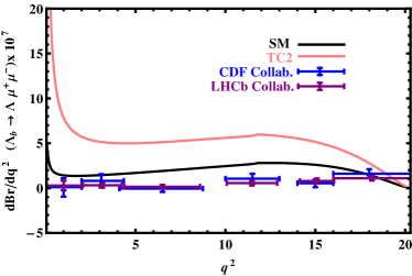
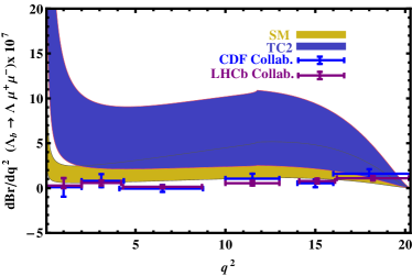
Figure 1: The dependence of the differential branching ratio (in $GeV^{-2}$ unit) on $q^{2}$ ($GeV^{2}$) for $\Lambda_{b}\rightarrow\Lambda\mu^{+}\mu^{-}$ decay channel in the SM and TC2 models using the central values of the form factors (left panel) and form factors with their uncertainties (right panel). The recent experimental results by CDF [1] and LHCb [2] are also presented in both figures.

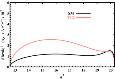
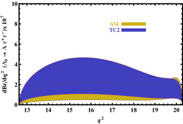
Figure 2: The dependence of the differential branching ratio (in $GeV^{-2}$ unit) on $q^{2}$ ($GeV^{2}$) for $\Lambda_{b}\rightarrow\Lambda\tau^{+}\tau^{-}$ decay channel in the SM and TC2 models using the central values of the form factors (left panel) and form factors with their uncertainties (right panel).

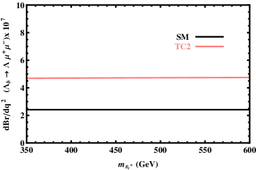
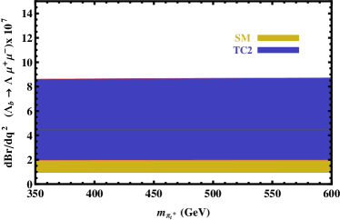
Figure 3: The dependence of the differential branching ratio (in $GeV^{-2}$ unit) on $m_{\pi_{t}^{+}}$ for $\Lambda_{b}\rightarrow\Lambda\mu^{+}\mu^{-}$ decay channel in the SM and TC2 models using the central values of the form factors (left panel) and form factors with their uncertainties (right panel).

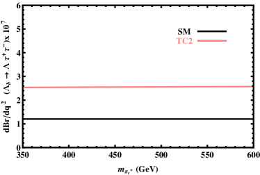
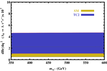
Figure 4: The same as figure 3 but for $\Lambda_{b}\rightarrow\Lambda\tau^{+}\tau^{-}$ decay channel.

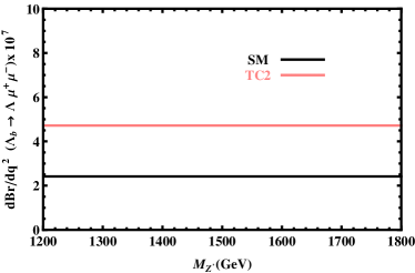
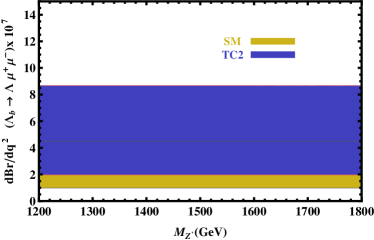
Figure 5: The dependence of the differential branching ratio (in $GeV^{-2}$ unit) on $M_{Z^{\prime}}$ for $\Lambda_{b}\rightarrow\Lambda\mu^{+}\mu^{-}$ decay channel in the SM and TC2 models using the central values of the form factors (left panel) and form factors with their uncertainties (right panel).

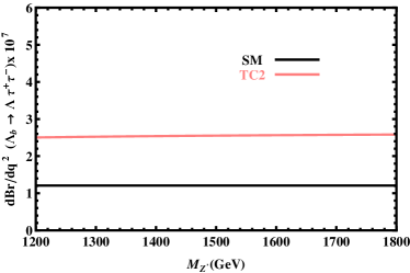
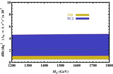
Figure 6: The same as figure 5 but for $\Lambda_{b}\rightarrow\Lambda\tau^{+}\tau^{-}$ decay channel.

To better compare the results, we depict the numerical values of the differential branching ratio at different values of $q^{2}$ in its allowed region for all lepton channels and both SM and TC2 models in Tables (5-7). We also present the experimental data in $\mu$ channel provided by the CDF [1] and LHCb [2] Collaborations in Table 5. With a quick glance in these tables, we see that

• in the case of $\mu$, the experimental data on the differential branching ratio especially those provided by the CDF Collaboration coincide/are close with/to the intervals predicted by the SM in all ranges of the $q^{2}$. Within the errors, the results of TC2 are consistent with the data by CDF Collaboration in the intervals $[2.00-4.30],~{}[10.09-12.86]$ and $[16.00-20.30]$ for the $q^{2}$ and with the data by LHCb Collaboration only for the interval $[16.00-20.30]$ for the $q^{2}$.

• In all lepton channels and within the errors, the intervals predicted by the TC2 model for the differential branching ratio coincide partly with the intervals predicted by the SM approximately in all ranges of the $q^{2}$.

These results show that although central values of the theoretical results differ considerably with the experimental data, considering the errors of form factors bring the intervals predicted by theory in both models close to the experimental data especially in the case of SM.

	SM	TC2	CDF [1]	LHCb [2]
$q^{2}$	$dBr/dq^{2}[10^{-7}]$	$dBr/dq^{2}[10^{-7}]$	$dBr/dq^{2}[10^{-7}]$	$dBr/dq^{2}[10^{-7}]$
$0.00-2.00$	$(0.60-2.58)$	$(3.29-14.36)$	$0.15\pm 2.01\pm 0.05$	$0.28\pm 0.38\pm 0.40\pm 0.06$
$2.00-4.30$	$(0.61-2.65)$	$(2.16-9.33)$	$1.84\pm 1.66\pm 0.59$	$0.31\pm 0.26\pm 0.07\pm 0.07$
$4.30-8.68$	$(0.80-3.48)$	$(2.17-9.31)$	$-0.20\pm 1.64\pm 0.08$	$0.15\pm 0.17\pm 0.02\pm 0.03$
$10.09-12.86$	$(1.11-4.93)$	$\small{(2.46-10.62)}$	$2.97\pm 1.47\pm 0.95$	$0.56\pm 0.21\pm 0.16\pm 0.12$
$14.18-16.00$	$(1.05-4.78)$	$(2.13-9.37)$	$0.96\pm 0.73\pm 0.31$	$0.79\pm 0.24\pm 0.15\pm 0.17$
$16.00-20.30$	$(0.54-2.57)$	$(1.06-4.84)$	$6.97\pm 1.88\pm 2.23$	$1.10\pm 0.18\pm 0.17\pm 0.24$

Table 5: Numerical values of the differential branching ratio in $GeV^{-2}$ for different intervals of $q^{2}$ ($GeV^{2}$) for $\Lambda_{b}\rightarrow\Lambda\mu^{+}\mu^{-}$ decay channel in SM and TC2 models obtained using the typical values of the masses $m_{\pi^{+}_{t}}=450~{}GeV$ and $M_{Z^{\prime}}=1500~{}GeV$. We also show the experimental values on the differential branching ratio provided by the CDF [1] and LHCb [2] Collaborations in this Table.

	SM	TC2
$q^{2}$	$dBr/dq^{2}[10^{-7}]$	$dBr/dq^{2}[10^{-7}]$
$0.00-2.00$	$(0.60-2.59)$	$(3.29-14.37)$
$2.00-4.30$	$(0.61-2.65)$	$(2.17-9.34)$
$4.30-8.68$	$(0.80-3.49)$	$(2.17-9.32)$
$10.09-12.86$	$(1.11-4.94)$	$(2.46-10.63)$
$14.18-16.00$	$(1.05-4.78)$	$(2.13-9.37)$
$16.00-20.30$	$(0.54-2.57)$	$(1.06-4.84)$

Table 6: Numerical values of the differential branching ratio in $GeV^{-2}$ for different intervals of $q^{2}$ ($GeV^{2}$) for $\Lambda_{b}\rightarrow\Lambda e^{+}e^{-}$ decay channel in SM and TC2 models obtained using the typical values of the masses $m_{\pi^{+}_{t}}=450~{}GeV$ and $M_{Z^{\prime}}=1500~{}GeV$.

	SM	TC2
$q^{2}$	$dBr/dq^{2}[10^{-7}]$	$dBr/dq^{2}[10^{-7}]$
$12.60-12.86$	$(0.11-0.53)$	$(0.28-1.22)$
$14.18-16.00$	$(0.47-2.15)$	$(1.05-4.61)$
$16.00-20.30$	$(0.43-1.96)$	$(0.77-3.46)$

Table 7: Numerical values of the differential branching ratio in $GeV^{-2}$ for different intervals of $q^{2}$ ($GeV^{2}$) for $\Lambda_{b}\rightarrow\Lambda\tau^{+}\tau^{-}$ decay channel in SM and TC2 models obtained using the typical values of the masses $m_{\pi^{+}_{t}}=450~{}GeV$ and $M_{Z^{\prime}}=1500~{}GeV$.

3.3 The branching ratio

In this part, we calculate the values of the branching ratio of the transition under consideration both in SM and TC2 models. For this aim, we need to multiply the total decay width by the lifetime of the initial baryon $\Lambda_{b}$ and divide by $\hbar$. Taking into account the typical values for $m_{\pi_{t}^{+}}$ and $M_{Z^{\prime}}$, we present the numerical results obtained from our calculations for both models together with the existing experimental data provided by the CDF [1] and LHCb [2] Collaborations in Table 8. As can be seen from this Table,

• although the central values of the branching ratios in TC2 model are roughly ($2-3.5$ times) bigger than those of the SM, adding the errors of form factors ends up in coinciding the intervals of the values predicted by the two models for all lepton channels.

• The orders of branching ratio show that the $\Lambda_{b}\rightarrow\Lambda\ell^{+}\ell^{-}$ decay can be accessible at the LHC for all leptons. As already mentioned, this decay at $\mu$ channel has been previously observed by the CDF and LHCb Collaborations.

• As it is expected, the value of the branching ratio decreases with increasing the mass of the final lepton.

• In the case of $\mu$ channel, the experimental data on the branching ratio coincide with the interval predicted by the SM within the errors, but these data considerably differ from the interval predicted by the TC2 model.

	$BR~{}(\Lambda_{b}\rightarrow\Lambda~{}e^{+}~{}e^{-})[10^{-6}]$	$BR~{}(\Lambda_{b}\rightarrow\Lambda~{}\mu^{+}~{}\mu^{-})[10^{-6}]$	$BR~{}(\Lambda_{b}\rightarrow\Lambda~{}\tau^{+}~{}\tau^{-})[10^{-6}]$
SM	$(1.81-8.06)$	$(1.64-7.30)$	$(0.34-1.51)$
TC2	$(6.62-29.03)$	$(4.55-19.81)$	$(0.63-2.77)$
CDF [1]	$-$	$1.73\pm 0.42\pm 0.55$	$-$
LHCb [2]	$-$	$0.96\pm 0.16\pm 0.13\pm 0.21$	$-$

Table 8: Numerical values of the branching ratio of $\Lambda_{b}\rightarrow\Lambda~{}\ell^{+}~{}\ell^{-}$ for $m_{\pi_{t}^{+}}=450~{}GeV$ and $M_{Z^{\prime}}=1500~{}GeV$ in SM and TC2 models together with the experimental data provided by the CDF [1] and LHCb [2] Collaborations.

In order to see how the TC2 model predictions deviate from those of SM, we plot the variations of branching ratios on $m_{\pi_{t}^{+}}$ and $M_{Z^{\prime}}$ in Figures 7-10. From these figures we see that

• there are big differences between the predictions of SM and TC2 models on branching ratio with respect to $m_{\pi_{t}^{+}}$ and $M_{Z^{\prime}}$ when the central values of the form factors are considered.

• The branching ratios remain approximately unchanged when the masses of $m_{\pi_{t}^{+}}$ and $M_{Z^{\prime}}$ are varied in the regions presented in the figures for both leptons.

• Adding the uncertainties of form factors ending up in intersections between the swept regions of two models, but can not totally kill the differences between two models predictions.

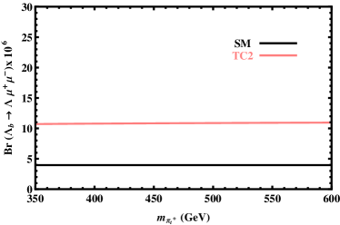
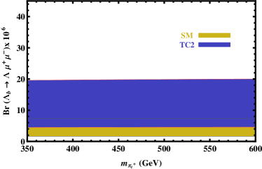
Figure 7: The dependence of the branching ratio on $m_{\pi_{t}^{+}}$ for $\Lambda_{b}\rightarrow\Lambda\mu^{+}\mu^{-}$ decay channel in the SM and TC2 models using the central values of the form factors (left panel) and form factors with their uncertainties (right panel).

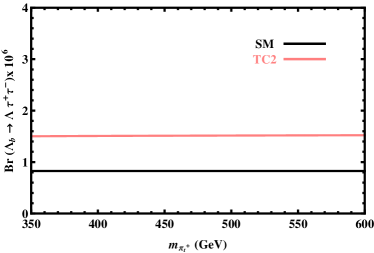
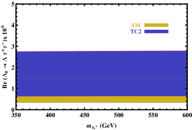
Figure 8: The same as figure 7 but for $\Lambda_{b}\rightarrow\Lambda\tau^{+}\tau^{-}$ transition.

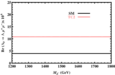
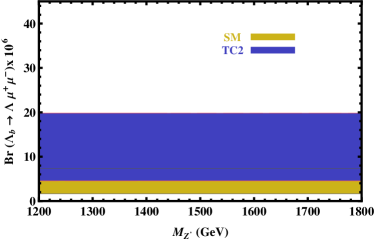
Figure 9: The same as figure 7 but with respect to $M_{Z^{\prime}}$.

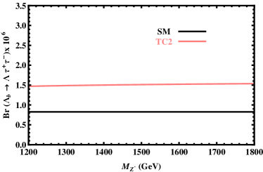
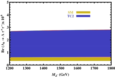
Figure 10: The same as figure 9 but for $\Lambda_{b}\rightarrow\Lambda\tau^{+}\tau^{-}$ transition.

3.4 The FBA

The present subsection embraces our analysis on the lepton forward-backward asymmetry (${\cal A}_{FB}$) in both the SM and TC2 models. The FBA is one of the most important tools to investigate the NP beyond the SM and it is defined as

$${\cal A}_{FB}(\hat{s})=\frac{\displaystyle{\int_{0}^{1}\frac{d\Gamma}{d\hat{s}dz}}(z,\hat{s})\,dz-\displaystyle{\int_{-1}^{0}\frac{d\Gamma}{d\hat{s}dz}}(z,\hat{s})\,dz}{\displaystyle{\int_{0}^{1}\frac{d\Gamma}{d\hat{s}dz}}(z,\hat{s})\,dz+\displaystyle{\int_{-1}^{0}\frac{d\Gamma}{d\hat{s}dz}}(z,\hat{s})\,dz}~{}.$$ (3.53)

The dependences of the FBA on $q^{2}$, $m_{\pi_{t}^{+}}$ and $M_{Z^{\prime}}$ for the decay under consideration in both $\mu$ and $\tau$ channels are depicted in Figures 11-16. A quick glance at these figures leads to the following results

• the effects of the uncertainties of form factors on ${\cal A}_{FB}$ are smaller compared to the differential branching ratio and branching ratio discussed in the previous figures.

• In Figure 11 where the dependence of ${\cal A}_{FB}$ on $q^{2}$ at $\mu$ channel is discussed, we see considerable differences between two models predictions at lower values of $q^{2}$ for both figures at left and right panels. At higher values of $q^{2}$, two models have approximately the same predictions. In $\tau$ case (Figure 12), two models have roughly the same results.

• In the case of ${\cal A}_{FB}$ in terms of $m_{\pi_{t}^{+}}$ and $\mu$ channel, the uncertainties of form factors end up in some common regions between two models predictions. In the case of $\tau$ channel, the difference between two models results exists even considering the uncertainties of form factors.

• In the case of ${\cal A}_{FB}$ on $M_{Z^{\prime}}$ and $\mu$ channel, we see a small difference between the SM and TC2 models predictions when the central values of form factors are considered. Taking into account uncertainties of form factors causes some intersections between two models predictions. In the case of $\tau$ (Figure 16), we see considerable discrepancies between two models predictions which can not be killed by the uncertainties of form factors.

• The ${\cal A}_{FB}$ is sensitive to $q^{2}$ for both leptons. The ${\cal A}_{FB}$ is also sensitive to $M_{Z^{\prime}}$ only for the case of $\tau$. However, this quantity remains roughly unchanged with respect to changes in $m_{\pi_{t}^{+}}$ for both lepton channels as well as with respect to $M_{Z^{\prime}}$ only for $\mu$ channel.

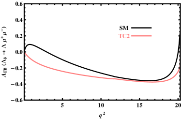
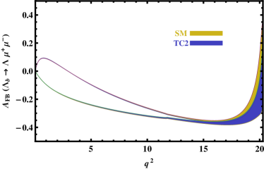
Figure 11: The dependence of the FBA on $q^{2}$ for $\Lambda_{b}\rightarrow\Lambda\mu^{+}\mu^{-}$ decay channel in the SM and TC2 models using the central values of the form factors (left panel) and form factors with their uncertainties (right panel).

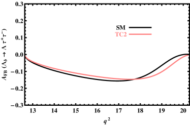
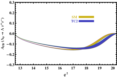
Figure 12: The same as figure 11 but for $\Lambda_{b}\rightarrow\Lambda\tau^{+}\tau^{-}$ decay channel.

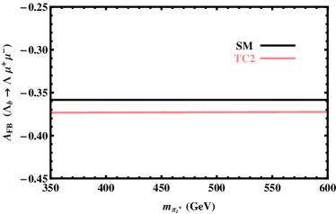
Figure 13: The same as figure 11 but with respect to $m_{\pi_{t}^{+}}$

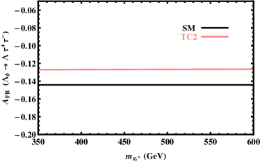
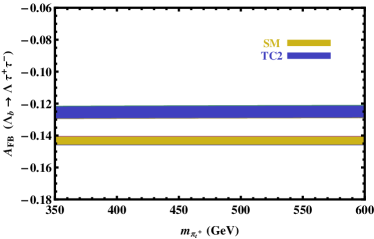
Figure 14: The same as figure 13 but for $\Lambda_{b}\rightarrow\Lambda\tau^{+}\tau^{-}$ decay channel.

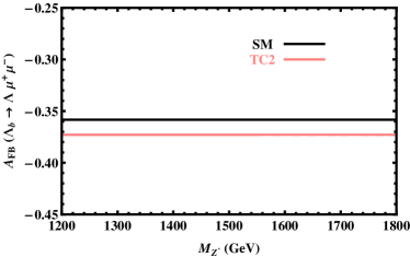
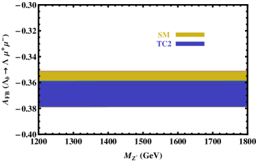
Figure 15: The same as figure 11 but with respect to $M_{Z^{\prime}}$.

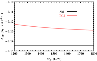
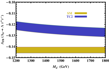
Figure 16: The same as figure 15 but for $\Lambda_{b}\rightarrow\Lambda\tau^{+}\tau^{-}$ decay channel.

4 Conclusion

In the present work, we have performed a comprehensive analysis of the baryonic FCNC $\Lambda_{b}\rightarrow\Lambda\ell^{+}\ell^{-}$ channel both in the SM and TC2 scenarios. In particular, we discussed the sensitivity of the differential branching ratio, branching ratio and lepton FBA on $q^{2}$ and the model parameters $m_{\pi_{t}^{+}}$ and $M_{Z^{\prime}}$ using the form factors calculated via light cone QCD sum rules as the main inputs. We saw overall considerable differences between two models’ predictions, which can not be totally killed by the uncertainties of form factors as the main sources of errors. However, the existing experimental data provided by the CDF and LHCb Collaborations in the case of differential branching ratio with respect to $q^{2}$ are very close to the SM results approximately in all ranges of $q^{2}$ when the errors of the form factors are considered. Only in some intervals of $q^{2}$, the experimental data on the differential branching ratio lie in the intervals predicted by the TC2 model within the errors. From the experimental side, we think we should have more data on different physical quantities defining the decay under consideration at different lepton channels as well as different baryonic and mesonic processes. This will help us in searching for NP effects especially those in the TC2 model as an alternative EWSB scenario to the Higgs mechanism.

5 Acknowledgement

We would like to thank Y. Erkuzu for her contribution in early stages of the calculations.

References

- [1] T. Aaltonen et al. [ CDF Collaboration ], “Observation of the Baryonic Flavor-Changing Neutral Current Decay ”, Phys. Rev. Lett. 107, 201802 (2011) [arXiv:1107.3753 [hep-ex]].
- [2] The LHCb Collaboration, “Measurement of the differential branching fraction of the decay ” [arXiv:1306.2577 [hep-ex]].
- [3] The ATLAS Collaboration, “Observation of a new particle in the search for the Standard Model Higgs boson with the ATLAS detector at the LHC”, Phys. Lett. B 716, 1 (2012) [arXiv:1207.7214 [hep-ex]].
- [4] The CMS Collaboration, “Observation of a new boson at a mass of 125 GeV with the CMS experiment at the LHC”, Phys. Lett. B 716, 30 (2012) [arXiv:1207.7235 [hep-ex]].
- [5] R. K. Kaul, “Technicolor”, Rev. Mod. Phys. 55, 449 (1983).
- [6] C. T. Hill, “Topcolor Assisted Technicolor”, Phys. Lett. B 345, 483 (1995) [arXiv:hep-ph/9411426].
- [7] K. Lane, E. Eichten, “Natural Topcolor–Assisted Technicolor”, Phys. Lett. B 352, 382 (1995) [arXiv:hep-ph/9503433].
- [8] D. Kominis, “Flavor-Changing Neutral Current Constraints in Topcolor-Assisted Technicolor”, Phys. Lett. B 358, 312 (1995) [arXiv:hep-ph/9506305].
- [9] Z. Xiao, W. Li, L. Guo, G. Lu, “Charmless decays , , and effects of new strong and electroweak penguins in Topcolor-assisted Technicolor model”, Eur. Phys. J. C 18, 681 (2001) [arXiv:hep-ph/0011175].
- [10] Z. Xiao, L. Guo, “Charmless hadronic decays in the Topcolor-assisted Technicolor model”, Commun. Theor. Phys. 40, 77 (2003) [arXiv:hep-ph/0306292].
- [11] W. Liu, C.-X. Yue, H.-D. Yang, “Rare decays and in the topcolor-assisted technicolor model”, Phys. Rev. D 79, 034008 (2009) [arXiv:0901.3463 [hep-ph]].
- [12] L.-X. Lü, X.-Q. Yang, Z.-C. Wang, “ decays in the topcolor-assisted technicolor model”, JHEP 1207, 157 (2012) [arXiv:1204.3361 [hep-ph]].
- [13] K. Lane, “A New Model of Topcolor-Assisted Technicolor”, Phys. Lett. B 433, 96 (1998) [arXiv:hep-ph/9805254].
- [14] C. T. Hill, E. H. Simmons, “Strong Dynamics and Electroweak Symmetry Breaking”, Phys. Rept. 381, 235 (2003); Erratum-ibid. 390, 553 (2004) [arXiv:hep-ph/0203079].
- [15] G. Cvetic, “Top quark condensation”, Rev. Mod. Phys. 71, 513 (1999) [arXiv:hep-ph/9702381].
- [16] G. Buchalla, G. Burdman, C.T. Hill, D. Kominis, “GIM Violation and New Dynamics of the Third Generation”, Phys. Rev. D 53, 5185 (1996) [arXiv:hep-ph/9510376].
- [17] H.-J. He, C.-P. Yuan, “New Method for Detecting Charged (Pseudo-)Scalars at Colliders”, Phys. Rev. Lett. 83, 28 (1999) [arXiv:hep-ph/9810367].
- [18] G. Burdman, “Scalars from Top-condensation Models at Hadron Colliders”, Phys. Rev. Lett. 83, 2888 (1999) [arXiv:hep-ph/9905347].
- [19] C. T. Hill, “Topcolor”, FERMILAB-CONF-97-032-T, September (1998) [arXiv:hep-ph/9702320].
- [20] G. Buchalla, A. J. Buras, M. E. Lautenbacher, “Weak Decays Beyond Leading Logarithms”, Rev. Mod. Phys. 68, 1125 (1996) [arXiv:hep-ph/9512380].
- [21] G. Bobeth, A. J. Buras, F. Krüger, J. Urban, “QCD Corrections to , , and in the MSSM”, Nucl. Phys. B 630, 87 (2002) [arXiv:hep-ph/0112305].
- [22] W. Altmannshofer, P. Ball, A. Bharucha, A. J. Buras, D. M. Straub, M. Wick, “Symmetries and Asymmetries of Decays in the Standard Model and Beyond”, JHEP 0901, 019 (2009) [arXiv: 0811.1214[hep-ph]].
- [23] A. Ghinculov, T. Hurth, G. Isidori, Y. P. Yao, “The rare decay to NNLL precision for arbitrary dilepton invariant mass”, Nucl. Phys. B 685, 351 (2004) [arXiv:hep-ph/0312128].
- [24] A. J. Buras, M. Misiak, M. Münz, S. Pokorski, “Theoretical Uncertainties and Phenomenological Aspects of Decay”, Nucl. Phys. B 424, 374 (1994) [arXiv:hep-ph/9311345].
- [25] M. Misiak, “The and decays with next-to-leading logarithmic QCD-corrections”, Nucl. Phys. B 393, 23 (1993); Erratum-ibid B 439, 161 (1995).
- [26] A. J. Buras, M. Muenz, “Effective Hamiltonian for Beyond Leading Logarithms in the NDR and HV Schemes”, Phys. Rev. D 52, 186 (1995) [arXiv:hep-ph/9501281].
- [27] A. J. Buras, “Weak Hamiltonian, CP Violation and Rare Decays”, C97-07-28, September 5 (1997) [arXiv:hep-ph/9806471].
- [28] Z. Xiao, C.-D. Lü, W. Huo, “Technicolor corrections on decays in QCD factorization”, Phys. Rev. D 67, 094021 (2003) [arXiv:hep-ph/0301221].
- [29] C.-X. Yue, J. Zhang, W. Liu, “Rare decays in the TC2 model and the LHT model”, Nucl. Phys. B 832, 342 (2010) [arXiv:1002.2010 [hep-ph]].
- [30] J. Beringer et al. (Particle Data Group), Phys. Rev. D 86, 010001 (2012).
- [31] T. M. Aliev, K. Azizi, M. Savci, “Analysis of the decay in QCD”, Phys. Rev. D 81, 056006 (2010) [arXiv:1001.0227 [hep-ph]].
- [32] T. Feldmann and M. W. Y. Yip, “Form Factors for Transitions in SCET”, Phys. Rev. D 85, 014035 (2012); Erratum-ibid. D 86, 079901 (2012) [arXiv:1111.1844 [hep-ph]].