Asymptotically AdS Charged Black Holes in String Theory with Gauss-Bonnet Correction in Various Dimensions

Abstract

We study charged black hole solutions in Einstein-Maxwell-Gauss-Bonnet theory with the dilaton field which is the low-energy effective theory of the heterotic string. The spacetime is $D$-dimensional and assumed to be static and plane symmetric with the $(D-2)$-dimensional constant curvature space and asymptotically anti-de Sitter. By imposing the boundary conditions of the existence of the regular black hole horizon and proper behavior at infinity where the Breitenlohner-Freedman bound should be satisfied, we construct black hole solutions numerically. We give the relations among the physical quantities of the black holes such as the horizon radius, the mass, the temperature, and so on. The properties of the black holes do not depend on the dimensions qualitatively, which is different from the spherically symmetric and asymptotically flat case. There is nonzero lower limit for the radius of the event horizon below which no solution exists. The temperature of the black hole becomes smaller as the horizon radius is smaller but remains nonzero when the lower limit is attained.

I Introduction

It is expected that quantum gravity plays the significant role in studying physics at strong gravity such as a black hole singularity. Since the ten-dimensional superstring theories or eleven-dimensional M-theory are the leading candidates for the quantum theory of gravity, it is interesting to use the low-energy effective theories of string/M theories to explore the problem. The effective theories are the supergravities which typically involve not only the metric but also the dilaton field (as well as several gauge fields). It is known that there are additional correction terms of higher orders in the curvature to the lowest effective supergravity action, the Gauss-Bonnet (GB) term coupled to the dilaton field in heterotic string MT .

When the dilaton field is set to a constant, the total action consists of the cosmological constant, Einstein-Hilbert and GB terms, which are the first three terms in the Lovelock theory Lovelock ; Zumino . There have been many works on the black hole solutions in the Lovelock theory GG ; KMR ; TYM ; CNO . Solutions in $D=4$ with GB term have been discussed in TYM . Boulware and Deser BD discovered static, spherically symmetric black hole solutions of such models in more than four dimensions. In the system with a negative cosmological constant, black holes can have horizons with nonspherical topology such as torus, hyperboloid, and other compactified submanifolds. These solutions were originally found in general relativity and are called topological black holes bro84 . Topological black hole solutions were studied also in the Einstein-GB theory Cai . However, the dilaton is not considered in most of the works. It is one of the important ingredients in string theory, so it is significant to study how its presence modifies the solutions. Unfortunately, it is not possible to find analytic solutions when the dilaton is present and is coupled to the GB term. We have to study this by numerical analysis. For related solutions, see TM ; BGO ; MOS1 ; CGOO ; MOS2 ; CGK ; MOW .

In a series of papers GOT1 ; GOT2 ; OT3 ; OT4 ; OT5 , we have studied neutral black hole solutions in the low-energy effective heterotic string, namely the Einstein theory plus the GB term coupled to the dilaton field MT . We have studied these solutions for asymptotically flat, anti-de Sitter (AdS) and de Sitter cases with suitable cosmological constants, and exhibited their properties including mass, temperature, entropy and their relations. These neutral solutions are useful for studying modifications of the black hole solutions by higher order effects induced by string theories. In particular, we have studied how the singularity may be modified and showed that they may be significantly modified. Also those solutions in AdS spacetime have been useful to study the corrections to the ratio of shear viscosity to entropy density vis ; CNOS .

Given this situation, it is natural to extend the black holes to charged ones. In our more recent paper OT6 , we have studied asymptotically flat charged black hole solutions in these theories. In fact, in the study of superconductors and superfluidity using the AdS/CFT correspondence, charged black hole solutions play important roles Gubser . Hence it is significant to extend our above asymptotically flat solutions to charged AdS ones. We should also consider the inclusion of the dilaton field. One of the purposes of this paper is to study asymptotically AdS charged black hole solutions with higher order corrections as well as the dilaton field.

There is another reason for our study of the solutions in such a system. In our above study of the neutral black holes GOT1 ; GOT2 ; OT3 ; OT4 ; OT5 , we did not consider the higher derivative term of the dilaton field. It is known, however, that such terms are also present in the effective theory MT . Hence we should incorporate this term as well and study how this modifies the solutions. We have studied this problem in the paper for asymptotically flat solutions OT6 , and found that there is not much qualitative difference. We will show that this is also true for the asymptotically AdS solutions. Thus the results in our earlier papers should be useful.

This paper is organized as follows. In Sec. II, we first present the action and give basic equations to solve for the system of Einstein-Maxwell-Gauss-Bonnet term (EMGB) coupled to the dilaton field with a cosmological constant. We then discuss symmetries which can be used to obtain solutions with different charge, mass and cosmological constant, given a solution for a charge, mass and cosmological constant. Boundary conditions and asymptotic behaviors are explored and parameter regions for the existence of the desired black hole solutions are determined. We show that the extreme black hole solutions with degenerate horizon can exist only when parameters take special values. In Sec. III, we choose the parameters for which we construct the black hole solutions, and discuss how the neutral solutions are modified in the presence of higher derivative terms of dilaton. Then the results for charged black holes are given and discussed for $D=4,5,6$ and 10. Section IV is devoted to conclusions and discussions.

II Dilatonic Einstein-Maxwell-Gauss-Bonnet theory

II.1 Action and basic equations

We consider the following low-energy effective action for the heterotic string theory in one scheme MT :

$$S = \frac{1}{2\kappa_{D}^{2}}\int d^{D}x\sqrt{-g}\Bigg{[}R-\frac{1}{2}(\partial\phi)^{2}-\frac{1}{4}e^{-\gamma\phi}F^{2}+\alpha_{2}e^{-\gamma\phi}\Big{\{}R^{2}_{\rm GB}+\frac{3}{16}(\partial\phi)^{4}\Big{\}}-\Lambda e^{\lambda\phi}\Bigg{]},$$ (1)

where $\kappa_{D}^{2}$ is a $D$-dimensional gravitational constant, $\phi$ a dilaton field, $F$ a gauge field strength, $\gamma=1/2$, $\alpha_{2}=\alpha^{\prime}/8$ is a numerical coefficient given in terms of the Regge slope parameter $\alpha^{\prime}$, $\lambda$ is a constant parameter, and $R^{2}_{\rm GB}=R_{\mu\nu\rho\sigma}R^{\mu\nu\rho\sigma}-4R_{\mu\nu}R^{\mu\nu}+R^{2}$ is the GB term. The field redefinition ambiguity MT ; MOW is applied to put the action into the above form. The three-form field $H_{\mu\nu\rho}$ is set to zero. This is allowed since it is a solution of the field equations. We investigated the neutral black hole solutions in the similar system without Maxwell field in Refs. GOT1 ; GOT2 ; OT3 ; OT4 ; OT5 . However, we did not take into account the higher order term of the dilaton field $(\partial\phi)^{4}$. Here we briefly discuss the modification due to this term as well as the charged solutions.

To construct black hole solutions, let us consider the metric and field strength:

$$ds_{D}^{2}=-B(r)e^{-2\delta(r)}dt^{2}+B(r)^{-1}dr^{2}+r^{2}h_{ij}dx^{i}dx^{j},~{}~{}F_{0r}=\frac{df(r)}{dr},$$ (2)

where $h_{ij}dx^{i}dx^{j}$ represents the line element of a $(D-2)$-dimensional constant curvature space with zero curvature and volume $\Sigma_{0}$.

The field equations following from the action (1) are

$$\bigl{(}B\tilde{r}^{D-3}\bigr{)}^{\prime}\frac{D-2}{\tilde{r}^{D-4}}h+\frac{1}{2}B\tilde{r}^{2}{\phi^{\prime}}^{2}+(D-1)_{4}\,e^{-\gamma\phi}\frac{B^{2}}{\tilde{r}^{2}}+4(D-2)_{3}\,\gamma e^{-\gamma\phi}B^{2}(\phi^{\prime\prime}-\gamma{\phi^{\prime}}^{2})$$

$$\hskip 14.22636pt-2(D-1)_{3}\,\gamma e^{-\gamma\phi}\phi^{\prime}\frac{B^{2}}{\tilde{r}}+\frac{\tilde{r}^{2}}{2}e^{2\delta-\gamma\phi}f^{\prime 2}-\frac{3}{16}B^{2}\tilde{r}^{2}e^{-\gamma\phi}\phi^{\prime 4}+\tilde{r}^{2}\tilde{\Lambda}e^{\lambda\phi}=0\,,~{}~{}$$ (3)

$$\delta^{\prime}(D-2)\tilde{r}h+\frac{1}{2}\tilde{r}^{2}{\phi^{\prime}}^{2}+2(D-2)_{3}\,\gamma e^{-\gamma\phi}B(\phi^{\prime\prime}-\gamma{\phi^{\prime}}^{2})-\frac{3}{8}\tilde{r}^{2}B\phi^{\prime 4}e^{-\gamma\phi}=0\,,$$ (4)

$$(e^{-\delta}\tilde{r}^{D-2}B\phi^{\prime})^{\prime} = \gamma(D-2)_{3}e^{-\gamma\phi-\delta}\tilde{r}^{D-4}\Big{[}(D-4)_{5}\frac{B^{2}}{\tilde{r}^{2}}+2(B^{\prime}-2\delta^{\prime}B)B^{\prime}+4B^{2}U(r)+4\frac{D-4}{\tilde{r}}(B^{\prime}-\delta^{\prime}B)B\Big{]}$$ (5)

$$+\gamma\tilde{r}^{D-2}e^{-\gamma\phi}\Big{(}\frac{1}{2}e^{\delta}f^{\prime 2}+\frac{3}{16}e^{-\delta}B^{2}\phi^{\prime 4}\Big{)}$$

$$+\frac{3}{4}\tilde{r}^{D-2}B\phi^{\prime 2}e^{-\delta-\gamma\phi}\Big{\{}3B\phi^{\prime\prime}+\Big{[}2B^{\prime}-\Big{(}\delta^{\prime}+\gamma\phi^{\prime}-\frac{D-2}{r}\Big{)}B\Big{]}\phi^{\prime}\Big{\}}+\tilde{r}^{D-2}\lambda\tilde{\Lambda}e^{-\delta+\lambda\phi},$$

$$(f^{\prime}e^{\delta-\gamma\phi}\tilde{r}^{D-2})^{\prime}=0,$$ (6)

where we have defined the dimensionless variables: $\tilde{r}=r/\sqrt{\alpha_{2}}$, $\tilde{\Lambda}=\alpha_{2}\Lambda$, and the primes in the field equations denote the derivatives with respect to $\tilde{r}$. Namely the length is measured in the unit of $\sqrt{\alpha_{2}}$. In what follows, we omit tilde on the variables for simplicity. We have also defined

$$(D-m)_{n} = (D-m)(D-m-1)(D-m-2)\cdots(D-n),$$

$$h = 1+2(D-3)e^{-\gamma\phi}\Big{[}-(D-4)\frac{B}{r^{2}}+\gamma\phi^{\prime}\frac{3B}{r}\Big{]},$$ (7)

$$\tilde{h} = 1+2(D-3)e^{-\gamma\phi}\Big{[}-(D-4)\frac{B}{r^{2}}+\gamma\phi^{\prime}\frac{2B}{r}\Big{]},$$ (8)

$$U(r) = (2\tilde{h})^{-1}\Bigg{[}-\frac{(D-3)_{4}}{r^{2}}-2\frac{D-3}{r}\Big{(}\frac{B^{\prime}}{B}-\delta^{\prime}\Big{)}-\frac{1}{2}\phi^{\prime 2}+(D-3)e^{-\gamma\phi}\Bigg{\{}(D-4)_{6}\frac{B}{r^{4}}$$ (9)

$$\hskip 28.45274pt+4(D-4)_{5}\frac{B}{r^{3}}\Big{(}\frac{B^{\prime}}{B}-\delta^{\prime}-\gamma\phi^{\prime}\Big{)}+4(D-4)\gamma\frac{B}{r^{2}}\Big{(}\gamma\phi^{\prime 2}+\frac{D-2}{r}\phi^{\prime}-\Phi\Big{)}$$

$$\hskip 28.45274pt+8\frac{\gamma\phi^{\prime}}{r}\biggl{[}\Big{(}\frac{B^{\prime}}{2}-\delta^{\prime}B\Big{)}\Big{(}\gamma\phi^{\prime}-\delta^{\prime}+\frac{2}{r}\Big{)}-\frac{D-4}{2r}B^{\prime}\biggr{]}+4(D-4)\Big{(}\frac{B^{\prime}}{2B}-\delta^{\prime}\Big{)}\frac{B^{\prime}}{r^{2}}-\frac{4\gamma}{r}\Phi(B^{\prime}-2\delta^{\prime}B)\Bigg{\}}$$

$$\hskip 28.45274pt+\frac{1}{2B}e^{2\delta-\gamma\phi}f^{\prime 2}+\frac{3}{16}B\phi^{\prime 4}e^{-\gamma\phi}-\frac{1}{B}{\Lambda}e^{\lambda\phi}\Biggr{]},$$

$$\Phi = \phi^{\prime\prime}+\Big{(}\frac{B^{\prime}}{B}-\delta^{\prime}+\frac{D-2}{r}\Big{)}\phi^{\prime}.$$ (10)

The original field equations involve the function $U(r)$ defined by

$$U(r)\equiv\Big{(}\frac{B^{\prime}}{2B}-\delta^{\prime}\Big{)}^{\prime}+\Big{(}\frac{B^{\prime}}{2B}-\delta^{\prime}\Big{)}^{2}+\frac{B^{\prime}}{2B}\Big{(}\frac{B^{\prime}}{2B}-\delta^{\prime}\Big{)}.$$ (11)

However in the field equations we have two equations involving $\delta^{\prime\prime}$, one of which can be used to eliminate $\delta^{\prime\prime}$ from $U(r)$ and obtain the expression (9). The resulting equations are the above set of equations with only the first derivative of $\delta$.

The field equation for the Maxwell field (6) is easily integrated to give

$$f^{\prime}=\frac{q}{r^{D-2}}e^{\gamma\phi-\delta},$$ (12)

where $q$ is a constant corresponding to the charge. So we can simply substitute this into our basic equations, and do not have to integrate the field equation for the Maxwell field simultaneously.

Our task is now reduced to setting boundary conditions for the metric functions $B,\>\delta$ and the dilaton field $\phi$, and integrate the above set of equations GOT1 ; GOT2 ; OT3 ; OT4 ; OT5 .

II.2 Symmetry and scaling

Before proceeding to the numerical analysis, it is useful to consider several symmetries of our field equations (or our model). First, our field equations (3)-(5) are invariant under the scaling transformation

$$B\to a^{2}B,~{}~{}r\to ar,~{}~{}q\to a^{D-2}q,$$ (13)

with an arbitrary nonzero constant $a$. If a black hole solution with the horizon radius $r_{H}$ is obtained, we can generate solutions with different horizon radii and charge but the same $\Lambda$ by this scaling transformation.

Second, there is the shift symmetry under

$$\phi\to\phi-\phi_{\ast},~{}~{}\Lambda\to e^{(\lambda-\gamma)\phi_{\ast}}\Lambda,~{}~{}B\to e^{-\gamma\phi_{\ast}}B,$$ (14)

where $\phi_{\ast}$ is an arbitrary constant. This changes the magnitude of the cosmological constant. Hence, given a solution with some value of the cosmological constant, this symmetry may be used to generate solutions for different values of the cosmological constant.

The final one is another shift symmetry under

$$\delta\to\delta-\delta_{\ast},~{}~{}t\to e^{-\delta_{\ast}}t,$$ (15)

with an arbitrary constant $\delta_{\ast}$, which may be used to shift the asymptotic value of $\delta$ to zero.

We will use these symmetries to obtain general black hole solutions after constructing solutions for given charge and cosmological constant.

II.3 Boundary conditions and asymptotic behaviors

In this paper we consider nonextreme solutions which have a nondegenerate black hole horizon. At the horizon $r_{H}$, we impose the conditions

$$B_{H}=0,~{}~{}B_{H}^{\prime}\neq 0,$$ (16)

where $B_{H}=B(r_{H})$. Here and in what follows, quantities evaluated at the horizon are represented by a subscript $H$. At the horizon, Eqs. (3)–(6) together with (7)–(12) give

$$B_{H}^{\prime} = -\frac{1}{D-2}\Big{[}r_{H}\Lambda e^{\lambda\phi_{H}}+\frac{q^{2}}{2r_{H}^{2D-5}}e^{\gamma\phi_{H}}\Big{]},$$ (17)

$$\phi_{H}^{\prime} = 2\gamma\frac{(D-2)_{3}}{r_{H}^{2}}e^{-\gamma\phi_{H}}B_{H}^{\prime}+\frac{1}{B_{H}^{\prime}}\Big{[}\lambda\Lambda e^{\lambda\phi_{H}}+\frac{\gamma q^{2}}{2r_{H}^{2D-4}}e^{\gamma\phi_{H}}\Big{]},$$ (18)

$$\delta_{H}^{\prime} = -\frac{1}{2(D-2)}r_{H}(\phi_{H}^{\prime})^{2}.$$ (19)

In the asymptotic region of $r\to\infty$, we assume

$$B \sim b_{2}r^{2}-\frac{2M}{r^{\mu}}+\cdots,$$

$$\delta \sim \delta_{0}+\frac{\delta_{1}}{r^{\sigma}}+\cdots,$$ (20)

$$\phi \sim \phi_{0}+\frac{\phi_{1}}{r^{\nu}}+\cdots,$$

with finite constants $b_{2}>0$, $M$, $\delta_{0}$, $\delta_{1}$, $\phi_{0}$, $\phi_{1}$ and positive constants $\mu$, $\sigma$, $\nu$; $b_{2}$ is related to the AdS radius.

In order to understand the asymptotic behaviors of our dilatonic system, it is convenient to study the “effective potential” for the dilaton. Its field equation can be written as

$$\kern 1.0pt\vbox{\hrule height=0.9pt\hbox{\vrule width=0.9pt\hskip 2.0pt\vbox{\vskip 5.5pt}\hskip 3.0pt\vrule width=0.3pt}\hrule height=0.3pt}\kern 1.0pt\phi=\frac{dV_{\rm eff}}{d\phi},$$ (21)

where the effective potential is defined by

$$V_{\rm eff}=-e^{-\gamma\phi}\Big{[}R_{\rm GB}^{2}+\frac{3}{16}(\partial\phi)^{4}-\frac{1}{4}F^{2}\Big{]}+\Lambda e^{\lambda\phi}.$$ (22)

A similar effective potential was analyzed in our earlier paper GOT2 for neutral AdS black holes in the absence of the Maxwell field and higher derivative term in the dilaton. Actually these additional contributions do not change the asymptotic behavior and we can take the results there. According to that analysis, we can have asymptotically AdS solutions only for $\lambda>0$. (The basic reason is that the potential (22) must have a maximum to which the dilaton $\phi$ tends at $r\to\infty$, and this is possible only for $\lambda>0$.) So hereafter we restrict our analysis to this case.

II.4 Asymptotic expansion

We now analyze the asymptotic behaviors of the solutions (see Ref. GOT2 ). Substituting the asymptotic behaviors (II.3) into the field equations (3) and (5) and using the original definition (11) of the function $U$, we require that the leading terms (proportional to $r^{2}$) should vanish. This gives

$$(D-1)_{4}e^{-\gamma\phi_{0}}b_{2}^{2}-(D-1)_{2}b_{2}-\Lambda e^{\lambda\phi_{0}}=0,$$ (23)

$$(D)_{3}\gamma e^{-\gamma\phi_{0}}b_{2}^{2}+\lambda\Lambda e^{\lambda\phi_{0}}=0,$$ (24)

which determine $b_{2}$ and $\phi_{0}$, while $\delta_{0}$ can be arbitrary due to the shift symmetry (15). Since $\gamma$ is positive and $\Lambda$ is negative, it follows from (24) that $\lambda$ should be positive in accordance to what we stated above. These are the same set of equations as in the neutral case GOT2 , and we can take the results from there. There we find that there are sensible solutions for $\lambda\neq\gamma$, to which we restrict our following discussions. Then Eqs. (23) and (24) give

$$b_{2}^{2} = -\frac{\lambda\Lambda}{(D)_{3}\gamma}\Big{[}\frac{D(D-3)}{(D-1)_{2}}(-\Lambda)\frac{\gamma}{\lambda}\Big{(}1+\frac{(D-4)\lambda}{D\gamma}\Big{)}^{2}\Big{]}^{(\gamma+\lambda)/(\gamma-\lambda)},$$ (25)

$$e^{\phi_{0}} = \Big{[}\frac{D(D-3)}{(D-1)_{2}}(-\Lambda)\frac{\gamma}{\lambda}\Big{(}1+\frac{(D-4)\lambda}{D\gamma}\Big{)}^{2}\Big{]}^{1/(\gamma-\lambda)}.$$ (26)

We find that the contributions from the field strength of the Maxwell field and the higher order dilaton terms are also subleading compared to other terms present in the neutral case, so the analysis of the next leading terms in Eqs. (3)–(5) is again completely the same as in Ref. GOT2 . Now let us summarize the results obtained there. First we have

$$(D-4)\lambda-D\gamma\neq 0,~{}~{}~{}~{}\mu=\nu-2=\sigma-2.$$ (27)

The asymptotic forms of the field functions are given by

$$B \sim b_{2}r^{2}-\frac{2M_{+}}{r^{\nu_{+}-2}}-\frac{2M_{0}}{r^{D-3}}+\cdots,$$

$$\delta \sim \frac{\delta_{+}}{r^{\nu_{+}}}+\cdots,$$ (28)

$$\phi \sim \phi_{0}+\frac{\phi_{+}}{r^{\nu_{+}}}+\cdots,$$

where we have set $\delta_{0}=0$ using the shift symmetry (15) and have defined

$$\nu_{\pm}=\frac{D-1}{2}\left(1\pm\sqrt{1-\frac{m^{2}}{m_{BF}^{2}}}\;\right),$$ (29)

and

$$m_{BF}^{2}\equiv-\frac{(D-1)^{2}}{4}b_{2},~{}~{}~{}m^{2}\equiv-\frac{(D)_{2}\lambda\gamma(\lambda-\gamma)[(D-4)\lambda+D\gamma]}{(D-4)^{2}\lambda^{2}-D^{2}\gamma^{2}-8(D-1)_{2}\lambda^{2}\gamma^{2}}b_{2}.$$ (30)

The mass square $m_{BF}^{2}$ is that of Breitenlohner and Freedman (BF) bound BF . In the asymptotic expansion of $\phi$ in (II.4), there would be a term $1/r^{\nu_{-}}$ in general, but we choose the boundary value $\phi_{H}$ such that this term is absent.

The function $B$ has the term $1/r^{\nu_{+}-2}$, but it can be shown that this term cancels out from the $g_{tt}$ component of the metric due to the condition that the next leading terms in the field equations cancel out (we have $M_{+}+b_{2}\delta_{+}=0$ from that condition, see Eq. (3.23) in Ref. GOT2 ). This leads to

$$g_{tt}=Be^{-2\delta}\sim b_{2}r^{2}-\frac{2M_{0}}{r^{D-3}}+\cdots.$$ (31)

This behavior is also confirmed by our numerical analysis. The value $M_{0}$ thus gives the gravitational mass of the black hole. Consequently it is convenient to define the mass function $m_{g}(r)$ by

$$-g_{tt}=b_{2}r^{2}-\frac{2m_{g}(r)}{r^{D-3}}.$$ (32)

We also have to impose the conditions

$$m^{2}<0,~{}~{}~{}\mbox{and}~{}~{}~{}m^{2}\geq m_{BF}^{2},$$ (33)

in order for our black hole solutions to exist and be stable. The first condition gives the allowed parameter regions

$$\lambda<\gamma,$$ (34)

or

$$\lambda>\frac{D\gamma}{\sqrt{(D-4)^{2}-8(D-1)_{2}\gamma^{2}}},~{}~{}~{}\mbox{and}~{}~{}~{}0<\gamma<\frac{D-4}{\sqrt{8(D-1)_{2}}}.$$ (35)

In constructing our black hole solutions, we choose the parameters in these regions.

Here we briefly comment on the extreme black hole solutions. At the degenerate horizon, where $B^{\prime}_{H}=0$, we have

$$r_{H}\Lambda e^{\lambda\phi_{H}}+\frac{q^{2}}{2r_{H}^{2D-5}}e^{\gamma\phi_{H}}=0,$$ (36)

by Eq. (17), and

$$\lambda\Lambda e^{\lambda\phi_{H}}+\frac{\gamma q^{2}}{2r_{H}^{2D-4}}e^{\gamma\phi_{H}}=0,$$ (37)

by the regularity of $\phi^{\prime}_{H}$ in Eq. (18). These equations give the conditions

$$\gamma=\lambda,~{}~{}~{}~{}~{}\Lambda+\frac{q^{2}}{2r_{H}^{2D-4}}=0.$$ (38)

When $\gamma=\lambda$, Eqs. (23) and (24) give

$$\Lambda=-\frac{(D)_{1}}{4(D-2)_{3}}.$$ (39)

These are the necessary conditions on the existence of the extreme solution. We thus see that the existence of the extreme black hole solutions depends on the very specific choice of parameters in our system and is not generic. Unless we make such a choice, we cannot have extreme solutions.

Let us also comment on the charge of the Maxwell field. By the existence of the cosmological constant $\Lambda$, the asymptotic value of the dilaton field is not zero but takes nonzero finite value $\phi_{0}$ determined by Eq. (26). This changes the coefficient of the field strength $f^{\prime}$ at infinity as $q\to qe^{-\gamma\phi_{0}}$. This means that the effective charge of the solution is $q_{\rm eff}=qe^{-\gamma\phi_{0}}$. We treat, however, the $q$ as the parameter of the solution in the following analysis.

II.5 Thermodynamical variables

The Hawking temperature is given by the periodicity of the Euclidean time on the horizon as

$$T_{H}\!\!\!\!\! =\frac{e^{-\delta_{H}}}{4\pi}B_{H}^{\prime}$$ (40)

$$=-\frac{e^{-\delta_{H}}}{4\pi(D-2)}\biggl{[}r_{H}\Lambda e^{\lambda\phi_{H}}+\frac{q^{2}e^{\gamma\phi_{H}}}{2r_{H}^{2D-5}}\biggr{]}.$$

Note that the cosmological constant is negative $\Lambda<0$, and the temperature becomes positive. Also this vanishes if extreme condition is satisfied.

Using the definition of entropy in the diffeomorphism invariant system in Ref. Wald , we obtain

$$S=-2\pi\int_{\Sigma}\frac{\partial{\cal L}}{\partial R_{\mu\nu\rho\sigma}}\epsilon_{\mu\nu}\epsilon_{\rho\sigma},$$ (41)

where $\Sigma$ is the event horizon $(D-2)$-surface, ${\cal L}$ is the Lagrangian density, $\epsilon_{\mu\nu}$ denotes the volume element binormal to $\Sigma$. This entropy has desirable properties such that it obeys the first law of black hole thermodynamics and that it is expected to obey even the second law Jacobson . For our present model, this gives

$$S=\frac{r_{H}^{D-2}\Sigma_{0}}{4}.$$ (42)

$\Sigma_{0}$ is the volume of the unit constant curvature space. This is the same form as the Bekenstein-Hawking entropy, i.e., a quarter of the horizon area.

III Numerical solutions of the dilatonic black holes

III.1 Parameters and scaling symmetry

We construct the black hole solutions numerically. For this purpose, we have to choose the parameters for our black hole solutions so as to satisfy the condition (33). We choose the following values as a typical example in various dimensions:

$$\gamma=\frac{1}{2},~{}~{}~{}\lambda=\frac{1}{3},~{}~{}~{}\delta_{0}=0,~{}~{}~{}\Lambda=-1,~{}~{}~{}q=1,~{}~{}~{}\phi_{-}=0.$$ (43)

The last condition $\phi_{-}=0$ means that the asymptotic behavior of $\phi$ in (II.4) is chosen such that the term like $1/r^{\nu_{-}}$ is absent. This is achieved by choosing suitable $\phi_{H}$. It should not be difficult to get solutions for other values of parameters in the allowed region.

We next fix the radius of the event horizon $r_{H}$, and choose the value of the dilaton field $\phi_{H}$ at the horizon, and determine the other fields by (17)-(19). Once a solution for one $r_{H}$, mass and charge is found, we can use the symmetry (13) to obtain other solutions by changing

$$r_{H}\to ar_{H},~{}~{}M_{0}\to a^{D-1}M_{0},~{}~{}q\to a^{D-2}q,$$ (44)

where $a$ is a constant parameter. Similarly, given a solution for a cosmological constant, we can generate solutions for different cosmological constants but the same $r_{H}$ and $q$ using transformation (14):

$$M_{0}\to b^{2\gamma/(\gamma-\lambda)}M_{0},~{}~{}\Lambda\to b^{2}\Lambda,~{}~{}\phi\to\phi+\frac{2}{\gamma-\lambda}\ln b,$$ (45)

with a constant parameter $b$.

III.2 Neutral black holes

Before proceeding to the charged solution which is the main issue of the paper, let us comment on the neutral solutions. Because the present system (1) includes the higher order term of the dilaton field $(\partial\phi)^{4}$, which is neglected in the previous analysis in Refs. GOT1 ; GOT2 ; OT3 ; OT4 ; OT5 , we should check how different our solutions may be from those without the higher order term. In the neutral case the following relation was derived by combining the symmetries (44) and (45):

$$M_{0}=m_{0}|\Lambda|^{\gamma/(\gamma-\lambda)}\>r_{H}^{\>D-1},$$ (46)

where $m_{0}$ is a coefficient.

We have constructed the neutral solutions numerically with the higher derivative term $(\partial\phi)^{4}$ included. Here we summarize the obtained values of the physical parameters in Table 1 for $D=4,\>5,\>6$, and 10. Since the solutions are qualitatively similar for dimensions beyond six, we do not give them explicitly, but $D=10$ is the critical dimension in superstring theories and is important for applications. The word “on” (“off”) in the column of $(\partial\phi)^{4}$ means that the higher order term of the dilaton field is (not) included. The values for “off” are those obtained in our previous paper GOT2 . It can be seen that the effect of the higher order term is tiny. The difference in the values of physical quantities becomes smaller as the dimension of the spacetime $D$ gets higher, and are less than 1% for all parameters in each dimensions. Hence we can conclude that the analysis in Ref. GOT2 is valid with enough accuracy.

Table 1: Values of the physical parameters of the neutral black hole solutions obtained by numerical calculations. The rows with $(\partial\phi)^{4}$ “on” (“off”) means that the higher order term of the dilaton field is (not) included. “off” case is obtained in GOT2 .

$D$	$(\partial\phi)^{4}$	$\phi_{H}$	$\delta_{H}$	$m_{0}$	$T$
4	off	$-$0.098566425	$-$0.028926580	0.08300	0.039632717
	on	$-$0.098650689	$-$0.028953439	0.08300	0.039632668
5	off	2.767015400	$-$0.021880831	0.14006	0.068192735
	on	2.766998583	$-$0.021886221	0.14006	0.068192721
6	off	4.154180204	$-$0.016209541	0.15948	0.080751210
	on	4.154175817	$-$0.016210949	0.15948	0.080751206
10	off	6.291642457	$-$0.002453368	0.13216	0.081203391
	on	6.291639521	$-$0.002453809	0.13216	0.081203348

III.3 Charged black holes

We now turn to the charged solutions. We fix the parameters as $r_{H}=1$, $q=1$ and $\Lambda=-1$. We then integrate the field equations (3)-(5) outward from the horizon numerically with the additional conditions  (17)-(19). By integrating the field equations with the value $\phi_{H}$, we have found that the dilaton field increases monotonically to $\phi_{0}$ at infinity.

With the parameters (43), we have constructed the black hole solutions and found $b_{2}$ and the asymptotic value of the dilaton field $\phi_{0}$. They are summarized in Table 2. These values do not depend on the charge $q$. For $D=4$, the asymptotic value of the dilaton field vanishes.

Table 2: The AdS curvature radius $b_{2}$ and the asymptotic value of the dilaton field $\phi_{0}$ for the parameter $\gamma=\frac{1}{2}$, $\lambda=\frac{1}{3}$, $\Lambda=-1$ in each dimension.

$D$	$b_{2}$	$\phi_{0}$
4	0.16667	0
5	1.50205	0.29147
6	0.24346	2.84082
10	0.15886	6.30143

Figures 1–4 show the relations $r_{H}$-$\phi_{H}$, $r_{H}$-$\delta_{H}$, $M_{0}$-$r_{H}$, and $r_{H}$-$T$ of the obtained black hole solutions in $D=4$, 5, 6 and 10, respectively. The solutions are shown for the charge $q=1$. By the scaling symmetries, these relations do not change if we make replacement $r_{H}\to r_{H}/q^{\frac{1}{D-2}}$, $M_{0}\to M_{0}/(|\Lambda|^{3}q^{\frac{D-1}{D-2}})$, $T\to T/(|\Lambda|^{3}q^{\frac{1}{D-2}})$, $\phi_{H}\to\phi_{H}-6\ln|\Lambda|$. $\delta_{H}$ is kept invariant under the symmetries. What this means is that if we replace the variables by this rule, these figures remain the same and we can get the relations among physical quantities including mass, horizon radius and temperature for the black hole solutions with other values of charges and cosmological constants. Those of the neutral solutions are also plotted for comparison. In particular, in diagrams (a) and (b) in Figs. 1–4, the blue horizontal lines show the values of $\phi_{H}$ and $\delta_{H}$ which are constant for neutral solutions and are given in Table 1. Their values for charged solutions asymptotically approach these values for neutral solutions because the effects of the charges become smaller for larger horizon radius $r_{H}$. To show precisely how $\phi_{H}$ and $\delta_{H}$ behaves near the horizontal line, we insert enlarged figures around there as an inset.

Figure 1: Various relations between the parameters for $D=4$ black hole solutions in (dilatonic) EMGB systems. (a) $r_{H}$-$\phi_{H}$ diagram (b) $r_{H}$-$\delta_{H}$ diagram (c) $M_{0}$-$r_{H}$ diagram (d) $r_{H}$-$T$ diagram. Thick (red) lines for the charged solutions with $q=1$ and thin (blue) lines for the neutral solutions. Below the dashed (green) curve in (c), there is no solution for any $q$.

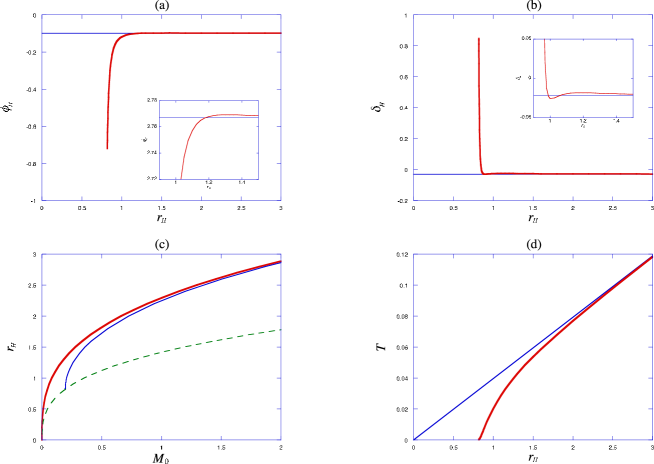
Figure 2: Various relations between the parameters for $D=5$ black hole solutions in (dilatonic) EMGB systems. (a) $r_{H}$-$\phi_{H}$ diagram (b) $r_{H}$-$\delta_{H}$ diagram (c) $M_{0}$-$r_{H}$ diagram (d) $r_{H}$-$T$ diagram. Thick (red) lines for the charged solutions with $q=1$ and thin (blue) lines for the neutral solutions. Below the dashed (green) curve in (c), there is no solution for any $q$.

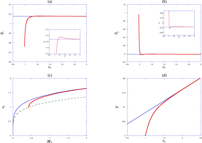
Figure 3: Various relations between the parameters for $D=6$ black hole solutions in (dilatonic) EMGB systems. (a) $r_{H}$-$\phi_{H}$ diagram (b) $r_{H}$-$\delta_{H}$ diagram (c) $M_{0}$-$r_{H}$ diagram (d) $r_{H}$-$T$ diagram. Thick (red) lines for the charged solutions with $q=1$ and thin (blue) lines for the neutral solutions. Below the dashed (green) curve in (c), there is no solution for any $q$.

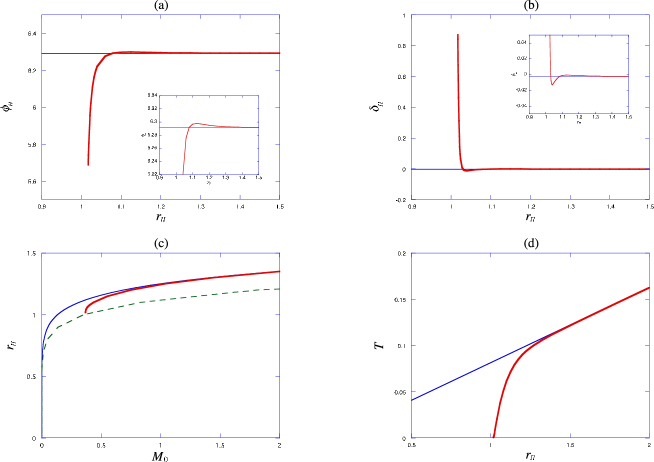
Figure 4: Various relations between the parameters for $D=10$ black hole solutions in (dilatonic) EMGB systems. (a) $r_{H}$-$\phi_{H}$ diagram (b) $r_{H}$-$\delta_{H}$ diagram (c) $M_{0}$-$r_{H}$ diagram (d) $r_{H}$-$T$ diagram. Thick (red) lines for the charged solutions with $q=1$ and thin (blue) lines for the neutral solutions. Below the dashed (green) curve in (c), there is no solution for any $q$.

Several features can be read off from the diagrams. Firstly we see that the qualitative behaviors of the diagrams do not depend on the dimensions $D$ much. For the neutral solutions, there are infinitesimally small black hole solutions in all dimensions as the horizon radius becomes small. This can be seen from the relation (46) in this case. The horizon becomes degenerate ($B_{H}^{\prime}\to 0$) and the temperature approaches zero in the limit of zero horizon radius. For the charged black holes away from the small horizon radius, mass and temperature similarly become smaller for smaller horizon. However, the situation drastically changes near small horizon radius and there is no such limit of zero horizon radius. There is nonzero lower limit for the radius of the event horizon below which no solution exists like Reissner-Nordström solution. However, the solution in the lower limit is not the extreme solution because it can exist only for $\lambda=\gamma$ as shown in (38), which is not satisfied here. The lower limits are found to be $r_{H}^{\ast}=0.8201,\;0.9491,\;0.9891,\;1.0173$ for $D=4,\;5,\;6,\;10$, respectively. Around these limits, the numerical calculation becomes unstable and it is difficult to say anything definite about the nature of this lower limit.

For $D=4$, $\phi_{H}$ is negative for all $r_{H}$, while it is positive for $D\geq 5$. $\phi_{H}$ becomes small rapidly as the horizon radius of the solution approaches the lower limit. On the other hand, $\delta_{H}$ increases sharply towards this limit. For the mass of the black hole, there is the lower limit $M_{0}^{\ast}=0.1940,\;0.360,\;0.426,\;0.368$ for $D=4,\;5,\;6,\;10$, respectively. From the data of the lower limit and the scaling symmetries, we find that the curve connecting the lower limits for each $q$ is

$$M_{0}^{\ast}=m^{\ast}|\Lambda|^{\gamma/(\gamma-\lambda)}\>{r_{H}^{\ast}}^{D-1}~{}~{}~{}(\;=m^{\ast}|\Lambda|^{3}\>{r_{H}^{\ast}}^{D-1}~{}\mbox{ for the choice~{}(\ref{para})}).$$ (47)

where $m^{\ast}=0.376,\;0.421,\;0.440,\;0.350$ for $D=4,\;5,\;6,\;10$, respectively. This is plotted by the dashed curves in the $M_{0}$-$r_{H}$ diagrams for any $q$. Below these curves there is no black hole solution. While the temperature seems to be zero in the lower limit in the $r_{H}$-$T$ diagrams, it is not the case. In fact the solutions at the lower limit have tiny but nonzero temperature $T^{\ast}=2.157\times 10^{-4},\;4.413\times 10^{-4},\;4.520\times 10^{-4},\;5.480\times 10^{-4}$ for $D=4,\;5,\;6,\;10$, respectively.

It is expected that the difference between charged and neutral solutions becomes small for large black holes, and this is confirmed in our solutions.

We have discussed qualitative properties of the black hole solutions. To evaluate actually physical quantities, it is necessary to have quantitative results. In order to get idea on what are the typical physical quantities, here we tabulate them for the black hole solutions in Table 3. The parameters change rapidly around the lower limit.

Table 3: Typical values of the physical quantities of the charged dilatonic black hole solutions for $\Lambda=-1$, $q=1$.

$D$	$r_{H}$	$M_{0}$	$\delta_{H}$	$\phi_{H}$	$\phi_{H}^{\prime}$	$T$
4	0.8201	0.194	0.8469	$-$0.7198	19.54	$2.157\times 10^{-4}$
	0.9	0.197	$-$0.03054	$-$0.1815	0.6084	0.009058
	1.0	0.205	$-$0.02611	$-$0.1097	0.1584	0.02001
	1.5	0.359	$-$0.02697	$-$0.09817	0.1913	0.05355
	2.0	0.725	$-$0.02826	$-$0.09835	0.1646	0.07678
5	0.9491	0.360	0.8358	2.159	25.21	$4.413\times 10^{-4}$
	1.0	0.364	$-$0.02594	2.671	1.058	0.01456
	1.2	0.446	$-$0.01857	2.768	0.08905	0.05991
	1.5	0.810	$-$0.02049	2.768	0.1403	0.09508
	2.0	2.298	$-$0.02161	2.767	0.1258	0.13467
6	0.9891	0.426	0.9610	3.520	34.30	$4.520\times 10^{-4}$
	1.0	0.426	0.1062	3.834	10.73	0.003386
	1.2	0.55	$-$0.01345	4.157	0.01678	0.07425
	1.4	0.96	$-$0.01495	4.156	0.08153	0.1053
	1.6	1.74	$-$0.01574	4.155	0.09288	0.1262
	1.8	3.06	$-$0.01602	4.154	0.08903	0.1440
10	1.0173	0.368	0.8703	5.688	63.624	$5.480\times 10^{-4}$
	1.1	0.438	$-$0.001355	6.297	$-$0.3420	0.06160
	1.15	0.552	$-$0.0008287	6.297	$-$0.3041	0.07914
	1.2	0.75	$-$0.001380	6.295	$-$0.2440	0.08992
	1.3	1.44	$-$0.002105	6.293	$-$0.1827	0.10330
	1.4	2.76	$-$0.002343	6.292	$-$0.1579	0.1129

IV Conclusions

In this paper we have studied asymptotically AdS charged black hole solutions in the dilatonic EMGB theory including the cosmological constant in various dimensions. The theory originates from the low-energy effective theory of the heterotic string. The spacetime is assumed to be static and plane symmetric, and should be regular outside of the black hole horizon. The system of the field equations has some symmetries which are used to obtain solutions with different masses and charges.

As the inner boundary conditions, we have assumed the existence of the regular black hole horizon. At infinity, the dilaton field decays fast enough for satisfying the BF bound for the stability. By these conditions, it is shown that the extreme black hole solution with degenerate horizon can exist only when the theoretical parameters satisfy very stringent conditions, and the existence of these is non-generic in the parameter space. Hence we only consider the solutions with non-degenerate horizon. The system of the field equations is complex so it is difficult to obtain an analytical solution. Hence we have investigated the solutions numerically.

Since the system in this paper includes the higher order term of the dilaton field, we have also analyzed the neutral solutions to see the difference from the solutions we obtained in Ref. GOT2 , which do not include such term. The numerical analysis shows that there is only difference less than 1% in the physical parameters between these solutions. The higher order term of the dilaton field does not much affect the solutions.

For the charged solutions, we have obtained the relations between the physical quantities (mass, temperature and horizon radius) for $D=4,5,6$ and 10. It is found that the properties of the solutions are qualitatively the same independently of the dimensions. We find that the mass and temperature become smaller for smaller horizon. However, there is a nonzero lower limit for the radius of the event horizon below which no solution exists. This is in sharp contrast to the neutral black holes where the horizon radius can go to zero together with the mass and temperature. We have shown the regions where no solution exists in the mass-horizon radius diagram. We have also confirmed that the difference between charged and neutral solutions becomes smaller for larger black holes.

With these solutions, we should be able to find corrections to those results obtained by applying the AdS/CFT correspondence to condensed matter physics. It would be extremely interesting to explore this direction.

References

- (1) R. R. Metsaev and A. A. Tseytlin, “Order alpha-prime (Two Loop) Equivalence of the String Equations of Motion and the Sigma Model Weyl Invariance Conditions: Dependence on the Dilaton and the Antisymmetric Tensor,” Nucl. Phys. B 293 (1987) 385.
- (2) D. Lovelock, “The Einstein tensor and its generalizations,” J. Math. Phys. 12 (1971) 498; “The four-dimensionality of space and the einstein tensor,” J. Math. Phys. 13 (1972) 874.
- (3) B. Zumino, “Gravity Theories in More Than Four-Dimensions,” Phys. Rept. 137 (1986) 109.
- (4) J. T. Wheeler, “Symmetric Solutions To The Gauss-Bonnet Extended Einstein Equations,” Nucl. Phys. B 268 (1986) 737; D. L. Wiltshire, Phys. Lett. B 169 (1986) 36; R. C. Myers and J. Z. Simon, “Black Hole Thermodynamics in Lovelock Gravity,” Phys. Rev. D 38 (1988) 2434; G. Giribet, J. Oliva and R. Troncoso, “Simple compactifications and black p-branes in Gauss-Bonnet and Lovelock theories,” JHEP 0605 (2006) 007 [arXiv:hep-th/0603177]; R. G. Cai and N. Ohta, “Black holes in pure Lovelock gravities,” Phys. Rev. D 74 (2006) 064001 [arXiv:hep-th/0604088]. For reviews and references, see C. Garraffo and G. Giribet, “The Lovelock Black Holes,” Mod. Phys. Lett. A 23 (2008) 1801 [arXiv:0805.3575 [gr-qc]] and C. Charmousis, “Higher order gravity theories and their black hole solutions,” Lect. Notes Phys. 769 (2009) 299 [arXiv:0805.0568 [gr-qc]].
- (5) P. Kanti, N. E. Mavromatos, J. Rizos, K. Tamvakis and E. Winstanley, “Dilatonic Black Holes in Higher Curvature String Gravity,” Phys. Rev. D 54 (1996) 5049 [arXiv:hep-th/9511071].
- (6) T. Torii, H. Yajima and K. -i. Maeda, “Dilatonic black holes with Gauss-Bonnet term,” Phys. Rev. D 55 (1997) 739 [gr-qc/9606034].
- (7) M. Cvetic, S. Nojiri and S. D. Odintsov, “Black hole thermodynamics and negative entropy in deSitter and anti-deSitter Einstein-Gauss-Bonnet gravity,” Nucl. Phys. B 628 (2002) 295 [arXiv:hep-th/0112045].
- (8) D. G. Boulware and S. Deser, “String Generated Gravity Models,” Phys. Rev. Lett. 55 (1985) 2656; “Effective Gravity Theories With Dilatons,” Phys. Lett. B 175 (1986) 409.
- (9) J. D. Brown, J. Creighton and R. B. Mann, “Temperature, energy and heat capacity of asymptotically anti-de Sitter black holes,” Phys. Rev. D 50 (1994) 6394 [gr-qc/9405007].
- (10) R. G. Cai, “Gauss-Bonnet black holes in AdS spaces,” Phys. Rev. D 65 (2002) 084014 [arXiv:hep-th/0109133].
- (11) T. Torii and H. Maeda, “Spacetime structure of static solutions in Gauss-Bonnet gravity: Neutral case,” Phys. Rev. D 71 (2005) 124002 [arXiv:hep-th/0504127]; Phys. Rev. D 72 (2005) 064007 [arXiv:hep-th/0504141].
- (12) K. Bamba, Z. K. Guo and N. Ohta, “Accelerating Cosmologies in the Einstein-Gauss-Bonnet Theory with Dilaton,” Prog. Theor. Phys. 118 (2007) 879 [arXiv:0707.4334 [hep-th]].
- (13) K. -i. Maeda, N. Ohta and Y. Sasagawa, “Black Hole Solutions in String Theory with Gauss-Bonnet Curvature Correction,” Phys. Rev. D 80 (2009) 104032 [arXiv:0908.4151 [hep-th]];
- (14) C. M. Chen, D. V. Gal’tsov, N. Ohta and D. G. Orlov, “Global solutions for higher-dimensional stretched small black holes,” Phys. Rev. D 81 (2010) 024002 [arXiv:0910.3488 [hep-th]].
- (15) K. -i. Maeda, N. Ohta and Y. Sasagawa, “AdS Black Hole Solution in Dilatonic Einstein-Gauss-Bonnet Gravity,” Phys. Rev. D 83 (2011) 044051 [arXiv:1012.0568 [hep-th]].
- (16) C. Charmousis, B. Gouteraux and E. Kiritsis, “Higher-derivative scalar-vector-tensor theories: black holes, Galileons, singularity cloaking and holography,” JHEP 1209 (2012) 011 [arXiv:1206.1499 [hep-th]].
- (17) K. -i. Maeda, N. Ohta and R. Wakebe, “Accelerating Universes in String Theory via Field Redefinition,” Eur. Phys. J. C 72 (2012) 1949 [arXiv:1111.3251 [hep-th]].
- (18) Z. K. Guo, N. Ohta and T. Torii, “Black Holes in the Dilatonic Einstein-Gauss-Bonnet Theory in Various Dimensions I – Asymptotically Flat Black Holes –,” Prog. Theor. Phys. 120 (2008) 581 [arXiv:0806.2481 [gr-qc]].
- (19) Z. K. Guo, N. Ohta and T. Torii, “Black Holes in the Dilatonic Einstein-Gauss-Bonnet Theory in Various Dimensions II – Asymptotically AdS Topological Black Holes –,” Prog. Theor. Phys. 121 (2009) 253 [arXiv:0811.3068 [gr-qc]].
- (20) N. Ohta and T. Torii, “Black Holes in the Dilatonic Einstein-Gauss-Bonnet Theory in Various Dimensions III – Asymptotically AdS Black Holes with –,” Prog. Theor. Phys. 121 (2009) 959 [arXiv:0902.4072 [hep-th]].
- (21) N. Ohta and T. Torii, “Black Holes in the Dilatonic Einstein-Gauss-Bonnet Theory in Various Dimensions IV - Topological Black Holes with and without Cosmological Term,” Prog. Theor. Phys. 122 (2009) 1477 [arXiv:0908.3918 [hep-th]].
- (22) N. Ohta and T. Torii, “Global Structure of Black Holes in String Theory with Gauss-Bonnet Correction in Various Dimensions,” Prog. Theor. Phys. 124 (2010) 207 [arXiv:1004.2779 [hep-th]].
-
(23)
A. Buchel and J. T. Liu,
“Universality of the shear viscosity in supergravity,”
Phys. Rev. Lett. 93 (2004) 090602
[arXiv:hep-th/0311175];
P. Kovtun, D. T. Son and A. O. Starinets, “Viscosity in strongly interacting quantum field theories from black hole physics,” Phys. Rev. Lett. 94 (2005) 111601 [arXiv:hep-th/0405231];
A. Buchel, J. T. Liu and A. O. Starinets, “Coupling constant dependence of the shear viscosity in N=4 supersymmetric Yang-Mills theory,” Nucl. Phys. B 707 (2005) 56 [arXiv:hep-th/0406264];
M. Brigante, H. Liu, R. C. Myers, S. Shenker and S. Yaida, “The Viscosity Bound and Causality Violation,” Phys. Rev. Lett. 100 (2008) 191601 [arXiv:0802.3318 [hep-th]]. - (24) R. -G. Cai, Z. -Y. Nie, N. Ohta and Y. -W. Sun, “Shear Viscosity from Gauss-Bonnet Gravity with a Dilaton Coupling,” Phys. Rev. D 79 (2009) 066004 [arXiv:0901.1421 [hep-th]].
- (25) N. Ohta and T. Torii, “Charged Black Holes in String Theory with Gauss-Bonnet Correction in Various Dimensions,” Phys. Rev. D 86 (2012) 104016 [arXiv:1208.6367 [hep-th]].
- (26) S. S. Gubser, “Breaking an Abelian gauge symmetry near a black hole horizon,” Phys. Rev. D 78 (2008) 065034 [arXiv:0801.2977 [hep-th]].
- (27) P. Breitenlohner and D. Z. Freedman, “Stability In Gauged Extended Supergravity,” Annals Phys. 144 (1982) 249.
-
(28)
R. M. Wald,
“Black hole entropy is the Noether charge,”
Phys. Rev. D 48 (1993) 3427
[arXiv:gr-qc/9307038];
V. Iyer and R. M. Wald, “Some properties of Noether charge and a proposal for dynamical black hole entropy,” Phys. Rev. D 50 (1994) 846 [arXiv:gr-qc/9403028]. - (29) T. Jacobson, G. Kang and R. C. Myers, “On black hole entropy,” Phys. Rev. D 49 (1994) 6587 [gr-qc/9312023]; “Increase of black hole entropy in higher curvature gravity,” Phys. Rev. D 52 (1995) 3518 [gr-qc/9503020].