Impact of E-ELT laser light on Cherenkov Telescope Array cameras

Abstract

As one of the options, the Cherenkov Telescope Array (CTA) Consortium is considering the possibility to install its Southern array in Chile, in the Atacama Desert. The envisaged site is situated about 5 km from the future European Extremely Large Telescope (E-ELT), which will operate 8 parallel DC lasers emitting at 589.2 nm, to create an artificial 6.8 magnitude star at an altitude of 90 km. The guide stars are used for the adaptive optics of the telescope. Although having the artificial stars in the field-of-view of a CTA telescope would happen rather seldom, and can be avoided by coordinated scheduling, the laser beams may cross the field-of-view of a telescope more frequently and leave spurious light tracks, hence complicating the analysis of the shower images. We derive an approximate formula to estimate the expected number of photons from molecular and aerosol scattering of the laser light beam into the field-of-view of a camera pixel. We then present several specific cases of laser influence on the CTA camera pixels, based on the selected direction of the laser beam, using the expected quantum efficiency of the camera photomultipliers at the given wavelength.

1 Introduction

Chile is now being considered seriously as a possible host country for the Southern array of the CTA  [1]. If accepted, the array would be installed in the Paranal - Cerro Armazones plateau, close to the location of the future European Extremely Large Telescope (E-ELT), which belongs to the European Southern Observatory (ESO). The most promising candidate site lies at a distance of about 5 km from the E-ELT, taking advantage of the infrastructure built for that installation. The E-ELT will operate 8 powerful DC lasers to create artificial guide-stars for the adaptive optics of its primary mirror. These lasers will operate at elevations of as low as 20^∘ and could therefore cross the field-of-view of the CTA telescopes nearby. The reflected laser light could then leave spurious light tracks in the cameras, affecting the analysis of the shower images or possibly triggering fake events.

We present here formulae to perform quick calculations for the amount of expected light from the laser beams in any of the CTA cameras, for a given distance to the E-ELT lasers and laser pointing angles. Inserting concrete values for typical case scenarios, and one absolutely worst case, will yield absolute numbers which can then be compared with other sources of background light, such as faint stars and/or the night-sky background.

2 The lasers

The E-ELT will operate 8 DC, extremely well collimated, lasers at a wavelength of 589.2 nm, each with a power of 20 W. The lasers will excite a layer of sodium atoms in the mesosphere (reaching about 90 km altitude a.s.l. for vertical shots) which then re-emit the laser-light and appear to “glow”. These so-called sodium laser guide stars most likely use circularly polarized laser light to achieve maximum impact [2]. The following table provides the relevant data:

Parameter	Value	Comments
Number of lasers	8	Fired in parallel
DC power	20 W	$5.9\cdot 10^{19}$ ph/s/laser
Max. distance	42 m
betw. lasers
Distance on ground	5 km	depends on exact
to the CTA		location of the CTA
Beam width	0.5 m
Beam opening	0.01 mrad
angle
Operation elevation	20–90∘	mostly above 45∘
Altitude	3 km a.s.l.

3 Scattering of the laser light

First, we consider Rayleigh scattering of light in dry air. Light of wavelength $\lambda$ and polarization angle $\phi$ is scattered by air molecules at a scattering angle $\theta$ with respect to the direction from which the photon impinges, with the following cross section [3]:

$$\frac{d\sigma(\phi,\theta,\lambda)}{d\Omega} = \frac{9\pi^{2}\cdot(n^{2}-1)^{2}}{\lambda^{4}\cdot N_{s}^{2}\cdot(n+2)^{2}}\cdot\big{(}\frac{6+3\rho}{6-7\rho}\big{)}\cdot$$ (1)

$$\cdot\big{(}\cos^{2}(\phi)\cos^{2}(\theta)+\sin^{2}(\phi)\big{)}~{}.$$

In the above formula, $N_{s}$ is the molecular concentration, $n$ the refractive index of air and $\rho$ the de-polarization ratio. Note that since $(n^{2}-1)/(n+2)$ is proportional to $N_{s}$, the resulting expression depends only on the particle mixture, and is independent of particle density as well as temperature and pressure [4]. Hence we can pick one reference condition for ($T,P$), which is typically made for the standard reference case $T_{s}=288.15$ K and $P_{s}=1013.25$ mbar.
$N_{s}$ is then $2.547\cdot 10^{25}$ m^-3. The combination $(n^{2}-1)/(n+2)$ yields $1.84\times 10^{-4}$ at $\lambda=589$ nm [5]. The King factor $(6+3\rho)/(6-7\rho)$ describes the effect of molecular anisotropy and amounts to about 1.05 [6]. Multiplying with the number density of molecules at a given height $h$, we obtain the volume scatter coefficient $\beta(\lambda,\theta,\phi,h)$:

$$\beta_{\mathrm{mol}}(589~{}\mathrm{nm},\theta,\phi,h) \approx 10^{-6}\cdot$$ (2)

$$\cdot\big{(}\cos^{2}(\phi)\cos^{2}(\theta)+\sin^{2}(\phi)\big{)}\cdot$$

$$\cdot\frac{N(h)}{N_{s}}~{}\mathrm{m^{-1}\,sr^{-1}}~{}.$$

Assuming un-polarized light, or a circularly polarized light beam seen over a field-of-view much larger than the wavenumber of a 589 nm light wave, the equation reduces to:

$$\beta_{\mathrm{mol}}(589~{}\mathrm{nm},\theta,h)\approx 10^{-6}\cdot\frac{\cos^{2}(\theta)+1}{2}\cdot\frac{N(h)}{N_{s}}~{}\mathrm{m^{-1}\,sr^{-1}}~{}.$$ (3)

We then consider a US standard troposphere [7] with:

$$\frac{N(h)}{N_{s}}\approx(1-2.3\cdot 10^{-5}\cdot h)^{4.256}~{}.$$ (4)

Aerosols scatter light more efficiently than molecules, due to their larger sizes. In order to reliably estimate the effect of aerosols on the scattering of the laser light, their size distribution and height dependency need to be known. We have not found any aerosol model for Paranal; however, the optical extinction has been described in great detail by [8]. Aerosol extinction at 589 nm is found to be $k_{\mathrm{aer}}(589~{}\mathrm{nm})=0.027\pm 0.004(\mathrm{stat.})\pm 0.004(\mathrm{syst.})$, where the systematic uncertainty represents the measured night-to-night variations. Since the AOD is an integral value over the entire troposphere, we further need a model for the height distribution of aerosols. First we consider that stratospheric aerosols contribute to $k_{\mathrm{strato}}=0.005$ to the measured aerosol extinction. Moreover, we can expect that at astronomical sites during the night only a nocturnal boundary layer of aerosols extends to about 2000 m above the ground, possibly showing residuals of the day-time planetary boundary layer at its edges. A fair approximation may be dividing the aerosol extinction by 2000 m to derive a constant aerosol extinction coefficient for heights from ground to 2000 m above it:

$$\beta_{\mathrm{aer}}(589~{}\mathrm{nm})_{\mathrm{tot}}\approx(1.0\pm 0.3)\cdot 10^{-5}~{}\mathrm{m^{-1}}~{}.$$ (5)

The extinction coefficient contains an absorption part and a scattering part; however, for continental clean environments, we can assume that more than 95% is due to scattering (i.e. the single scattering albedo is greater than 0.95). Furthermore, we can use the Henyey-Greenstein formula [9] to estimate the angular distribution of scattered light:

$$\beta_{\mathrm{aer}}(589~{}\mathrm{nm},\theta) \approx (1.0\pm 0.3)\cdot 10^{-5}\cdot\frac{1-g^{2}}{4\pi}\cdot$$ (6)

$$\bigg{(}\frac{1}{(1+g^{2}-2g\cos\theta)^{3/2}}+$$

$${}+f\frac{3\cos^{2}\theta-1}{2\cdot(1+g^{2})^{3/2}}\bigg{)}~{}\mathrm{m^{-1}}~{},$$

where $g$ varies between 0 and 1 and represents the mean value of $\cos(\theta)$. The parameter $f$ characterizes the strength of the second component to the backward scattering peak. Typical values for clear atmospheres and desert environments are $g\approx 0.6,f\approx 0.4$ [10]. Inserting these numbers, we obtain a very approximate expression for the aerosol volume scattering cross section, valid if the laser light is observed at heights below $\sim$2 km above ground:

$$\beta_{\mathrm{aer}}(589~{}\mathrm{nm},\theta) \approx (3.3\pm 1.0)\cdot 10^{-7}\cdot$$ (7)

$$\cdot\bigg{(}\frac{1}{(1-\cos\theta)^{3/2}}+$$

$${}+0.19\cdot(3\cos\theta-1)\bigg{)}~{}\mathrm{m^{-1}}~{}.$$

Contrary to the Rayleigh scattering case on molecules, this value can show large variations, depending on atmospheric conditions. For instance, a layer of haze can dramatically increase the aerosol scattering cross section, while scattering at heights above 2 km will probably result in a negligible contribution.

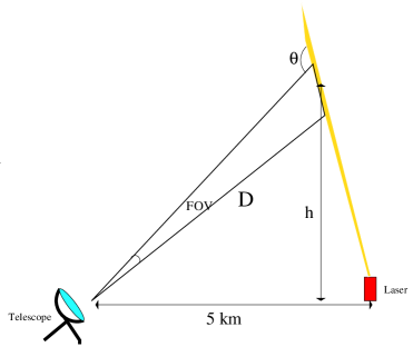
Fig. 1: Sketch of the chosen geometry conventions.

4 Amount of spurious light in individual CTA pixels

We can now derive the amount of light observed by a single pixel, assuming that the camera of a CTA telescope observes the laser beam at an angle $\theta$ with respect to the optical axis of the telescope, defined such that if both laser and telescope optical axes are parallel, then $\theta=\pi$, if the axes cross perpendicularly, then $\theta=\pi/2$ (see figure 1). Moreover, the laser is sufficiently collimated that the observed beam width is always smaller than the pixel FOV. The pixel will then observe a part of the laser track, corresponding to its field-of-view (FOV):

$$d_{\mathrm{track}}=\frac{\textit{FOV}_{\mathrm{pix}}\cdot D}{\sin(\theta)}~{},$$ (8)

where $D$ is the distance of the telescope to the laser beam at the place where the optical axis and the beam cross. The observed photon flux inside one laser’s track is:

$$N_{\mathrm{laser}}=\frac{P_{\mathrm{laser}}\cdot\lambda}{h\,c}\approx 5.9\cdot 10^{19}\quad\mathrm{s^{-1}}~{}.$$ (9)

Assuming that $D$ is large, we can approximate the scattering angle as constant throughout the crossing of the beam through the FOV of the pixel. The observed laser track will scatter into a solid angle $\Omega=A_{\mathrm{tel}}/D^{2}$, where $A_{\mathrm{tel}}$ is the area of the telescope mirror. Assuming a photo-multiplier quantum efficiency (QE) at 589 nm $\textit{QE}_{589\,\mathrm{nm}}$ and a combined reflection and photo-electron (phe) collection efficiency of $\xi\sim 0.9$, we obtain:

$$N_{\mathrm{pixel}} \approx N_{\mathrm{laser}}\cdot\xi\cdot\textit{QE}_{589\,\mathrm{nm}}\cdot\frac{A_{\mathrm{tel}}}{D^{2}}\cdot\frac{\textit{FOV}_{\mathrm{pix}}\cdot D}{\sin(\theta)}$$ (10)

$$\cdot\big{(}\beta_{\mathrm{mol}}(589~{}\mathrm{nm},\theta,h)+\beta_{\mathrm{aer}}(589~{}\mathrm{nm},\theta,h)\big{)}$$

$$\approx 8.2\cdot 10^{13}\cdot\textit{QE}_{589\,\mathrm{nm}}\cdot\frac{\textit{FOV}_{\mathrm{pix}}\cdot A_{\mathrm{tel}}}{D\cdot\sin(\theta)}\cdot$$

$$\cdot\bigg{(}\big{(}0.32-7.4\cdot 10^{-6}\cdot H\big{)}^{4.256}\cdot(\cos^{2}\theta+1)+$$

$$+(1-\Theta(h,2~{}\mathrm{km}))\cdot\big{(}\frac{0.21}{(1-\cos\theta)^{3/2}}+$$

$${}+0.04\cdot(3\cos\theta-1)\big{)}\bigg{)}~{}\mathrm{s^{-1}}~{},$$

where $\Theta(x)$ is the Heaviside function, $H$ is the altitude of the scattering point, i.e. 3 km, and $h$ the height above ground at which the laser is observed.

Eq. 10 allows us to draw the following preliminary conclusions:

1. Those cameras will be affected most which have the highest combination of $\textit{FOV}_{\mathrm{pix}}\cdot A_{\mathrm{tel}}\cdot\textit{QE}_{589\,\mathrm{nm}}$.

2. Although the function $(1-\cos^{2}(\theta))/\sin(\theta)$ has a (divergent) maximum at $\theta=0$, i.e. parallel beams, this does not mean that a laser beam parallel to the optical telescope axis will yield the highest (back)scatter return. Since we have neglected the reduction of the solid angle with increasing distance, this is an artificial effect of Eq. 10. However, at $\theta=0.9\pi$, $(1-\cos^{2}(\theta))/\sin(\theta)$ has only increased by a factor of two, suggesting that Eq. 10 is at least not valid for viewing angles higher than that value.

3. Apart from the effect described in point 2, the distance $D$ to the laser beam reduces the amount of registered light linearly. This is due to the combination of reduced solid angle (which goes with $D^{-2}$) and the increased part of the track spanned by the FOV of a pixel (which goes with $D$, due to the one-dimensional propagation of the laser beam).

5 Case scenarios

The following table gives an overview of the relevant parameters of each CTA camera under consideration:

Camera	Mirror area	Pixel FOV	$A\cdot$FOV
	(m2)	(mrad)	$(\mathrm{m}^{2}\cdot\mathrm{rad})$
LST	415	1.7	0.71
MST-DC	113	3	0.34
MST-SC	$\sim$50	1.17	0.06
SST-DC	12.5	4.14	0.05
SST-SC	$\sim$6	2.9	0.02

One can see that the highest spurious signal is expected for the LSTs, except the distance from one MST to the laser beam is a factor two smaller than the one from the LSTs. The E-ELT lasers are located at a distance of 5 km from the CTA, but the largest distance that an MST can have w.r.t. the LSTs, is only 1 km, the worst-case distance of an MST to E-ELT would be 4 km. Since the effect of a decrease in distance by a factor 0.8 is much less than an increase of $A\cdot\textit{FOV}$ by a factor 2.1, we consider only the LST case further.

Worst case scenario We remark that this scenario is highly improbable to happen. The laser is shooting at 70^∘ zenith angle towards the CTA, the LSTs are looking into the direction of the laser, at 20^∘ zenith angle. The distance to the laser beam is then as low as 1700 m, scattering occurs at 4500 m a.s.l., aerosol scattering takes place and increases the amount of scattered light. In this case, the scattering angle $\theta$ is 90 degrees and:

$$N_{\mathrm{pixel}}=(13\pm 3)\cdot\textit{QE}_{589\,\mathrm{nm}}\cdot N_{\mathrm{lasers}}~{}~{}\mathrm{ph.e./ns}~{},$$ (11)

However, in this case, the beam will likely appear broader in the camera, since seen out of focus. Therefore, the amount of light will appear rather distributed among a row of two to three pixels.

A typical bad case Both ELT and the CTA observe at 45^∘ zenith angle, with the laser pointing towards the CTA. The distance to the laser beam is then 3500 m, scattering occurs at 5500 m a.s.l., aerosol scattering can be disregaded. In this case, the scattering angle $\theta$ is again 90 degrees and:

$$N_{\mathrm{pixel}}=3.3\cdot\textit{QE}_{589\,\mathrm{nm}}\cdot N_{\mathrm{lasers}}~{}~{}\mathrm{ph.e./ns}~{},$$ (12)

A typical good case. The CTA observes at 30^∘ zenith angle, the lasers pointing upwards. The distance to the laser beam is then 10000 m, scattering occurs at 11700 m a.s.l., aerosol scattering can be disregarded. In this case, the scattering angle $\theta$ is 120 degrees and:

$$N_{\mathrm{pixel}}=0.8\cdot\textit{QE}_{589\,\mathrm{nm}}\cdot N_{\mathrm{lasers}}~{}~{}\mathrm{ph.e./ns}~{},$$ (13)

Figure 2 shows the equivalent $B$ star magnitude in one pixel vs. the photomultiplier QE at the laser wavelength. The magnitudes have been derived assuming the flux of Vega from [11] and a common photomultiplier $\mathrm{QE}_{440\,\mathrm{nm}}=0.35$ at 440 nm wavelength, and a spectral width of the QE of $d\lambda/\lambda=0.2$. A global atmospheric extinction of $z=0.25$ is further assumed for the $B$-filter.

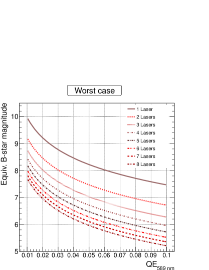
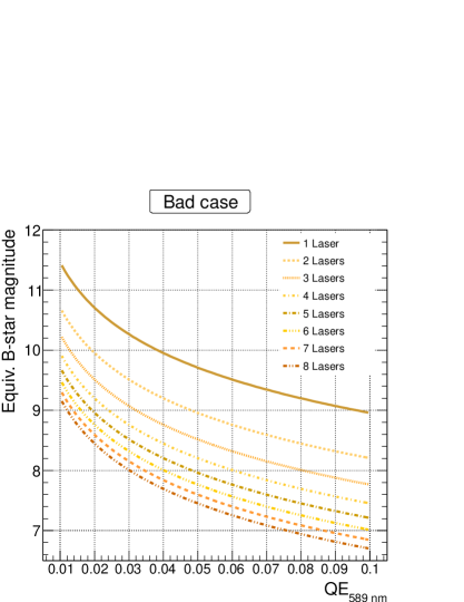
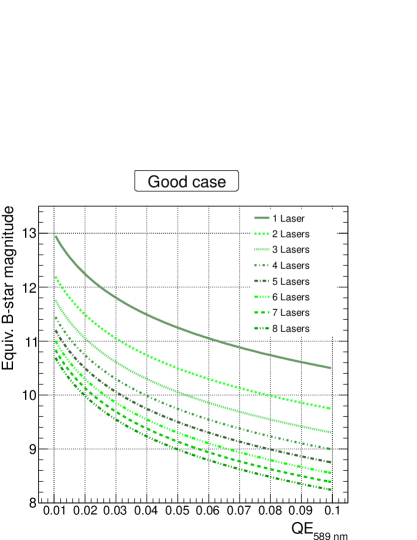
Fig. 2: Equivalent star $B$-magnitude for LST pixels for different QE values at 589 nm, and for three different pointing scenarios. The different lines represent the number of lasers observed at the same time in one camera pixel.

6 Discussion and Conclusions

We expect from negotiations with the provider that the QEs of the photomultipliers, used for the LST, will oscillate between roughly 2% and 7% at 590 nm wavelength. While the night sky background at the Chilean site is expected to produce roughly 0.2 phe/ns per LST pixel, the expected signal seen from an E-ELT lasers for a typical good case is 0.02 phe/ns in the case of photo-multipliers with less than 2% QE at 589 nm and 0.06 phe/ns for the case of 7% QE. In this situation, the laser photons should not affect data significantly, since their amount is much lower than the light-of-night sky. The typical bad case, together with 2% QE, corresponds to the typical good case with 7% QE and should still be acceptable, both in terms of spurious islands in the image and in terms of fake triggers. This possibility is rather small, since the ultra-collimated laser light is seen far from the telesopes, and should hit pixels in one single row. Therefore any next-neighbor logic of the trigger, if applied, should reject these events.

However, having rows of 8^m stars throughout the camera, as would typical for the bad case with 7% QE, could compromise the analysis already and should be avoided. A completely different case is the absolute worst case situation: here, we can get more than an order of magnitude higher phe-fluxes than the night-sky background, and the images would be strongly affected. Both cases should be avoided, but should not occur frequently, since the E-ELT lasers must point to low elevations, and towards the CTA for this to occur.

Another possible solution would be to exclude the pixels in the camera hit by the laser light in the reconstruction software, given that the laser direction should be known at any moment. Since the laser light is received during each shower event, the track can affect the direction and energy reconstruction of the event.

If the numbers plugged into formula 10 are correct, i.e. if the core of CTA lies at least 5 km from the site of the E-ELT, and if LST QEs are below 7% at 589 nm (better even $<2$%), and not more than 8 lasers are fired synchronously at the E-ELT, then the effect of the laser tracks in the CTA cameras should be sufficiently small in typical situations that it will not compromise trigger rates and image reconstruction.

Only the bad and worst case situation will have an effect on the recorded images and should be avoided, especially if the photo-multiplier QE is higher than 2% at 589 nm. The worst case (E-ELT lasers pointing at very low elevation towards CTA), must be avoided. However, this should happen so rarely that it can probably be avoided by coordinated scheduling.

Acknowledgements: We gratefully acknowledge support from the agencies and organizations listed in this page: http://www.cta-observatory.org/?q=node/22.

References

- [1] Acharya, B.S. et al., Astrop. Phys, 43 (2013) pp. 3–18.
- [2] Holzlöhner R., Rochester S. M., Bonaccini Calia D., Budker D., Higbie J. M. and Hackenberg W., A&A 510 (2010) A20.
- [3] Penndorf, R., J. of the Opt. Soc. of America 47 (1957) pp. 176-182.
- [4] Bodhaine, B. A., Am. Meteor. Soc. 16 (1999) pp. 1854-1861.
- [5] Peck E. R. and Reeder K., J. of the Opt. Soc. of America 62 (1972) pp. 958-962.
- [6] Tomasi, C. et al., Applied Optics 44 (2005) p. 3320.
- [7] U.S. Standard Atmosphere, NOAA Document S/T 76-1562 (1976).
- [8] Patat, F. et al., A&A 527 (2011) A91.
- [9] Henyey L. G. and Greenstein J. L., Astrophys. J. 93 (1941) pp. 70-83.
- [10] Louedec K. and Losno R., Eur. Phys. J. Plus 127 (2012) p. 97, arXiv:1208.6275.
- [11] Bohlin R., ASP Conference Series 999 (2007), astro-ph/0608715v1.