QuickXsort: Efficient Sorting with $n\log n-1.399n+o(n)$ Comparisons on Average

Abstract

In this paper we generalize the idea of QuickHeapsort leading to the notion of QuickXsort. Given some external sorting algorithm X, QuickXsort yields an internal sorting algorithm if X satisfies certain natural conditions.

With QuickWeakHeapsort and QuickMergesort we present two examples for the QuickXsort-construction. Both are efficient algorithms that incur approximately $n\log n-1.26n+o(n)$ comparisons on the average. A worst case of $n\log n+\mathcal{O}(n)$ comparisons can be achieved without significantly affecting the average case.

Furthermore, we describe an implementation of MergeInsertion for small $n$. Taking MergeInsertion as a base case for QuickMergesort, we establish a worst-case efficient sorting algorithm calling for $n\log n-1.3999n+o(n)$ comparisons on average. QuickMergesort with constant size base cases shows the best performance on practical inputs: when sorting integers it is slower by only 15% to STL-Introsort.

1 Introduction

Sorting a sequence of $n$ elements remains one of the most frequent tasks carried out by computers. A lower bound for sorting by only pairwise comparisons is $\left\lfloor\mathinner{\log n!}\right\rfloor\approx n\log n-1.44n+\mathcal{O}(\log n)$ comparisons for the worst and average case (logarithms referred to by $\log$ are base 2, the average case refers to a uniform distribution of all input permutations assuming all elements are different).

Sorting algorithms that are optimal in the leading term are called constant-factor-optimal. Table 1 lists some milestones in the race for reducing the coefficient in the linear term. One of the most efficient (in terms of number of comparisons) constant-factor-optimal algorithms for solving the sorting problem is Ford and Johnson’s MergeInsertion algorithm [7]. It requires $n\log n-1.329n+\mathcal{O}(\log n)$ comparisons in the worst case [10]. MergeInsertion has a severe drawback that makes it uninteresting for practical issues: similar to Insertionsort the number of element moves is quadratic in $n$. With Insertionsort we mean the algorithm that inserts all elements successively into the already ordered sequence finding the position for each element by binary search (not by linear search as mostly done). However, MergeInsertion and Insertionsort can be used to sort small subarrays such that the quadratic running time for these subarrays is small in comparison to the overall running time.

Reinhardt [12] used this technique to design an internal Mergesort variant that needs in the worst case $n\log n-1.329n+\mathcal{O}(\log n)$ comparisons. Unfortunately, implementations of this InPlaceMergesort algorithm have not been documented. Katajainen et al.’s [9, 6] work inspired by Reinhardt is practical, but the number of comparisons is larger.

Throughout the text we avoid the terms in-place or in-situ and prefer the term internal (opposed to external). We call an algorithm internal if it needs at most $\mathcal{O}(\log n)$ space in addition to the array to be sorted. That means we consider Quicksort as an internal algorithm whereas standard Mergesort is external because it needs a linear amount of extra space.

Based on QuickHeapsort [1], in this paper we develop the concept of QuickXsort and apply it to other sorting algorithms as Mergesort or WeakHeapsort. This yields efficient internal sorting algorithms. The idea is very simple: as in Quicksort the array is partitioned into the elements greater and less than some pivot element. Then one part of the array is sorted by some algorithm X and the other part is sorted recursively. The advantage of this procedure is that, if X is an external algorithm, then in QuickXsort the part of the array which is not currently being sorted may be used as temporary space, what yields an internal variant of X. We show that under natural assumptions QuickXsort performs up to $o(n)$ terms on average the same number of comparisons as X.

Table 1: Constant-factor-optimal sorting with $n\log n+\kappa n+o(n)$ comparisons.

	Mem.	Other	$\kappa$ Worst	$\kappa$ Avg.	$\kappa$ Exper.
Lower bound	$\mathcal{O}(1)$	$\mathcal{O}(n\log n)$	-1.44	-1.44
BottomUpHeapsort [13]	$\mathcal{O}(1)$	$\mathcal{O}(n\log n)$	$\omega(1)$	–	[0.35,0.39]
WeakHeapsort [3, 5]	$\mathcal{O}(n/w)$	$\mathcal{O}(n\log n)$	0.09	–	[-0.46,-0.42]
RelaxedWeakHeapsort [4]	$\mathcal{O}(n)$	$\mathcal{O}(n\log n)$	-0.91	-0.91	-0.91
Mergesort [10]	$\mathcal{O}(n)$	$\mathcal{O}(n\log n)$	-0.91	-1.26	–
ExternalWeakHeapsort #	$\mathcal{O}(n)$	$\mathcal{O}(n\log n)$	-0.91	-1.26*	–
Insertionsort [10]	$\mathcal{O}(1)$	$\mathcal{O}(n^{2})$	-0.91	-1.38 #	–
MergeInsertion [10]	$\mathcal{O}(n)$	$\mathcal{O}(n^{2})$	-1.32	-1.3999 #	[-1.43,-1.41]
InPlaceMergesort [12]	$\mathcal{O}(1)$	$\mathcal{O}(n\log n)$	-1.32	–	–
QuickHeapsort [1, 2]	$\mathcal{O}(1)$	$\mathcal{O}(n\log n)$	$\omega(1)$	-0.03	$\approx$ 0.20
	$\mathcal{O}(n/w)$	$\mathcal{O}(n\log n)$	$\omega(1)$	-0.99	$\approx$ -1.24
QuickMergesort (IS) #	$\mathcal{O}(\log n)$	$\mathcal{O}(n\log n)$	-0.32	-1.38	–
QuickMergesort #	$\mathcal{O}(1)$	$\mathcal{O}(n\log n)$	-0.32	-1.26	[-1.29,-1.27]
QuickMergesort (MI) #	$\mathcal{O}(\log n)$	$\mathcal{O}(n\log n)$	-0.32	-1.3999	[-1.41,-1.40]

Abbreviations: # in this paper, MI MergeInsertion, – not analyzed, * for $n=2^{k}$, $w$: computer word width in bits; we assume $\log n\in\mathcal{O}(n/w)$.

For QuickXsort we assume InPlaceMergesort as a worst-case stopper (without $\kappa_{\mathrm{worst}}\in\omega(1)$).

The concept of QuickXsort (without calling it like that) was first applied in UltimateHeapsort by Katajainen [8]. In UltimateHeapsort, first the median of the array is determined, and then the array is partitioned into subarrays of equal size. Finding the median means significant additional effort. Cantone and Cincotti [1] weakened the requirement for the pivot and designed QuickHeapsort which uses only a sample of smaller size to select the pivot for partitioning. UltimateHeapsort is inferior to QuickHeapsort in terms of average case running time, although, unlike QuickHeapsort, it allows an $n\log n+\mathcal{O}(n)$ bound for the worst case number of comparisons. Diekert and Weiß [2] analyzed QuickHeapsort more thoroughly and showed that it needs less than $n\log n-0.99n+o(n)$ comparisons in the average case when implemented with approximately $\sqrt{n}$ elements as sample for pivot selection and some other improvements.

Edelkamp and Stiegeler [4] applied the idea of QuickXsort to WeakHeapsort (which was first described by Dutton [3]) introducing QuickWeakHeapsort. The worst case number of comparisons of WeakHeapsort is $n\lceil\log n\rceil-2^{\lceil\log n\rceil}+n-1\leq n\log n+0.09n$, and, following Edelkamp and Wegener [5], this bound is tight. In [4] an improved variant with $n\log n-0.91n$ comparisons in the worst case and requiring extra space is presented. With ExternalWeakHeapsort we propose a further refinement with the same worst case bound, but in average requiring approximately $n\log n-1.26n$ comparisons. Using ExternalWeakHeapsort as X in QuickXsort we obtain an improvement over QuickWeakHeapsort of [4].

As indicated above, Mergesort is another good candidate to apply the QuickXsort-construction. With QuickMergesort we describe an internal variant of Mergesort which not only in terms of number of comparisons is almost as good as Mergesort, but also in terms of running time. As mentioned before, MergeInsertion can be used to sort small subarrays. We study MergeInsertion and provide an implementation based on weak heaps. Furthermore, we give an average case analysis. When sorting small subarrays with MergeInsertion, we can show that the average number of comparisons performed by Mergesort is bounded by $n\log n-1.3999n+o(n)$, and, therefore, QuickMergesort uses at most $n\log n-1.3999n+o(n)$ comparisons in the average case.

2 QuickXsort

In this section we give a more precise description of QuickXsort and derive some results concerning the number of comparisons performed in the average and worst case. Let X be some sorting algorithm. QuickXsort works as follows: First, choose some pivot element as median of some random sample. Next, partition the array according to this pivot element, i. e., rearrange the array such that all elements left of the pivot are less or equal and all elements on the right are greater or equal than the pivot element. Then, choose one part of the array and sort it with algorithm X. (In general, it does not matter whether the smaller or larger half of the array is chosen. However, for a specific sorting algorithm X like Heapsort, there might be a better and a worse choice.) After one part of the array has been sorted with X, move the pivot element to its correct position (right after/before the already sorted part) and sort the other part of the array recursively with QuickXsort.

The main advantage of this procedure is that the part of the array that is not being sorted currently can be used as temporary memory for the algorithm X. This yields fast internal variants for various external sorting algorithms (such as Mergesort). The idea is that whenever a data element should be moved to the external storage, instead it is swapped with some data element in the part of the array which is not currently being sorted. Of course, this works only, if the algorithm needs additional storage only for data elements. Furthermore, the algorithm has to be able to keep track of the positions of elements which have been swapped. As the specific method depends on the algorithm X, we give some more details when we describe the examples for QuickXsort.

For the number of comparisons we can derive some general results which hold for a wide class of algorithms X. Under natural assumptions the average case number of comparisons of X and of QuickXsort differs only by an $o(n)$-term. For the rest of the paper, we assume that the pivot is selected as the median of approximately $\sqrt{n}$ randomly chosen elements. Sample sizes of approximately $\sqrt{n}$ are likely to be optimal as the results in [2, 11] suggest.

Theorem 1 (QuickXsort Average-Case).

Let X be some sorting algorithm requiring at most $n\log n+cn+o(n)$ comparisons in the average case. Then, QuickXsort implemented with $\Theta(\sqrt{n})$ elements as sample for pivot selection is a sorting algorithm that also needs at most $n\log n+cn+o(n)$ comparisons in the average case.

For the proofs we assume that the arrays are indexed starting with $1$. The following lemma is crucial for our estimates. It can be derived by applying Chernoff bounds or by direct elementary calculations.

Lemma 1 ([2, Lm. 2]).

Let $0<\delta<\frac{1}{2}$. If we choose the pivot as median of $2\gamma+1$ elements such that $2\gamma+1\leq\frac{n}{2}$, then we have $\mathop{\mathrm{Pr}}\left[\,\text{pivot }\leq\frac{n}{2}-\delta n\,\right]<(2\gamma+1)\alpha^{\gamma}$ where $\alpha=4\left(\frac{1}{4}-\delta^{2}\right)<1$.

Proof of Thm. 1.

Let $T(n)$ denote the average number of comparisons performed by QuickXsort on an input array of length $n$ and let $S(n)=n\log n+cn+s(n)$ with $s(n)\in o(n)$ be an upper bound for the average number of comparisons performed by the algorithm X on an input array of length $n$. Without loss of generality we may assume that $s(n)$ is monotone. We are going to show by induction that

$$T(n)\leq n\log n+cn+t(n)$$

for some monotonically increasing $t(n)\in o(n)$ with $s(n)\leq t(n)$ which we will specify later.

Let $\delta(n)\in o(1)\cap\Omega(n^{-\frac{1}{4}+\epsilon})$ with $1/n\leq\delta(n)\leq 1/4$, i. e., $\delta$ is some function tending slowly to zero for $n\to\infty$. Because of $\delta(n)\in\Omega(n^{-\frac{1}{4}+\epsilon})$, we see that $(2\gamma+1)\left(1-4\delta^{2}\right)^{\gamma}$ tends to zero if $\gamma\in\Theta(\sqrt{n})$. Hence, by Lem. 1 it follows that the probability that the pivot is more than $n\cdot\delta(n)$ off the median $p(n)=\mathop{\mathrm{Pr}}\left[\,\text{pivot }<n\left(\frac{1}{2}-\delta(n)\right)\,\right]+\mathop{\mathrm{Pr}}\left[\,\text{pivot }>n\left(\frac{1}{2}+\delta(n)\right)\,\right]$ tends to zero for $n\to\infty$. In the following we write $M=\left[n\left(\frac{1}{2}-\delta(n)\right),n\left(\frac{1}{2}+\delta(n)\right)\right]\cap\mathbb{N}$ and $\overline{M}=\{1,\dots,n\}\setminus M$. We obtain the following recurrence relation:

$$T(n) \leq n-1+T_{\mathrm{pivot}}(n)$$

$$\qquad+\sum_{k=1}^{n}\mathop{\mathrm{Pr}}\left[\,\!\text{pivot }=k\!\,\right]\cdot\max\left\{\,T(k-1)+S(n-k),T(n-k)+S(k-1)\,\right\}$$

$$\leq n-1+T_{\mathrm{pivot}}(n)$$

$$\qquad+\mathop{\mathrm{Pr}}\left[\,\!\text{pivot }\in M\!\,\right]\cdot\max_{k\in M}\left\{\,T(k)+S(n-k),T(n-k)+S(k)\,\right\}$$

$$\qquad+\mathop{\mathrm{Pr}}\left[\,\!\text{pivot }\in\overline{M}\!\,\right]\cdot\max_{k\in\overline{M}}\left\{\,T(k)+S(n-k),T(n-k)+S(k)\,\right\}.$$

The function $f(x)=x\log x+(n-x)\log(n-x)$, $f(0)=f(n)=n\log n$ has its only minimum in the interval $[0,n]$ at $x=n/2$, i. e., for $0<x<n/2$ it decreases monotonically and for $n/2<x<n$ it increases monotonically. We set $\beta=\left(\frac{n}{2}+n\cdot\delta(n)\right)$. That means that we have $f(x)\leq f(\beta)$ for $x\in M$ and $f(x)\leq f(n)$ for $x\in\overline{M}$. Using this observation, the induction hypothesis, and our assumptions, we conclude

$$\max_{k\in M}\left\{\,T(k)+S(n-k),T(n-k)+S(k)\,\right\}$$

$$\qquad\leq\max\left\{\,\mathinner{f(k)+cn+t(k)+s(n-k)}\vphantom{k\in M}\>\left|\>\vphantom{f(k)+cn+t(k)+s(n-k)}\mathinner{k\in M}\right.\,\right\}\leq f(\beta)+cn+t(\beta)+s(n),$$

$$\max_{k\in\overline{M}}\left\{\,T(k)+S(n-k),T(n-k)+S(k)\,\right\}$$

$$\qquad\leq\max\left\{\,\mathinner{f(k)+cn+t(k)+s(n-k)}\vphantom{k\in\overline{M}}\>\left|\>\vphantom{f(k)+cn+t(k)+s(n-k)}\mathinner{k\in\overline{M}}\right.\,\right\}\leq T(n)+s(n).$$

With $p(n)$ as above we obtain:

$$\begin{split}T(n)&\leq n-1+T_{\mathrm{pivot}}(n)+p(n)\cdot T(n)+s(n)\\ &\qquad+(1-p(n))\bigl{(}f(\beta)+cn+t(\beta)\bigr{)}.\end{split}$$ (1)

We subtract $p(n)\cdot T(n)$ on both sides and then divide by $1-p(n)$. Let $D$ be some constant such that $D\geq 1/(1-p(n))$ for all $n$ (which exists since $p(n)\neq 1$ for all $n$ and $p(n)\to 0$ for $n\to\infty$). Then, we obtain

$$T(n) \leq\left(1+D\cdot p(n)\right)\cdot(n-1)+D\cdot(T_{\mathrm{pivot}}(n)+s(n))+\bigl{(}f(\beta)+cn+t(\beta)\bigr{)}$$

$$\leq\left(1+D\cdot p(n)\right)\cdot(n-1)+D\cdot(T_{\mathrm{pivot}}(n)+s(n))$$

$$\qquad+\left(\frac{n}{2}-n\cdot\delta(n)\right)\cdot(\log(n/2)+\log(1+2\delta(n)))$$

$$\qquad+\left(\frac{n}{2}+n\cdot\delta(n)\right)\cdot(\log(n/2)+\log(1+2\delta(n)))+cn+t(3n/4)$$

$$\leq n\log n+cn$$

$$\qquad+\left(D\cdot p(n)+2\cdot\delta(n)/\ln 2\right)\cdot n+D\cdot(T_{\mathrm{pivot}}(n)+s(n))+t(3n/4),$$

where the last inequality follows from $\log(1+x)=\ln(1+x)/\ln(2)\leq x/\ln(2)$ for $x\in\mathbb{R}_{>0}$. We see that $T(n)\leq n\log n+cn+t(n)$ if $t(n)$ satisfies the inequality

$$\left(D\cdot p(n)+2\cdot\delta(n)/\ln 2\right)\cdot n+D\cdot\left(T_{\mathrm{pivot}}(n)+s(n)\right)+t(3n/4)\leq t(n).$$

We choose $t(n)$ as small as possible. Inductively, we can show that for every $\epsilon$ there is some $D_{\epsilon}$ such that $t(n)<\epsilon n+D_{\epsilon}$. Hence, the theorem follows. ∎

Does QuickXsort provide a good bound for the worst case? The obvious answer is “no”. If always the $\sqrt{n}$ smallest elements are chosen for pivot selection, a running time of $\Theta(n^{3/2})$ is obtained. However, we can prove that such a worst case is very unlikely. In fact, let $R(n)$ be the worst case number of comparisons of the algorithm X. Prop. 1 states that the probability that QuickXsort needs more than $R(n)+6n$ comparisons decreases exponentially in $n$. (This bound is not tight, but since we do not aim for exact probabilities, Prop. 1 is enough for us.)

Proposition 1.

Let $\epsilon>0$. The probability that QuickXsort needs more than $R(n)+6n$ comparisons is less than $(3/4+\epsilon)^{\sqrt[4]{n}}$ for $n$ large enough.

Proof.

Let $n$ be the size of the input. We say that we are in a good case if an array of size $m$ is partitioned in the interval $[m/4,\,3m/4]$, i. e., if the pivot is chosen in that interval. We can obtain a bound for the desired probability by estimating the probability that we always are in such a good case until the array contains only $\sqrt{n}$ elements. For smaller arrays, we can assume an upper bound of $\sqrt{n}^{2}=n$ comparisons for the worst case. For all partitioning steps that sums up to less than $n\cdot\sum_{i\geq 0}(3/4)^{i}=4n$ comparisons if we are always in a good case. We also have to consider the number of comparisons required to find the pivot element. At any stage the pivot is chosen as median of at most $\sqrt{n}$ elements. Since the median can be determined in linear time, for all stages together this sums up to less than $n$ comparisons if we are always in a good case and $n$ is large enough. Finally, for all the sorting phases with X we need at most $R(n)$ comparisons in total (that is only a rough upper bound which can be improved as in the proof of Thm. 1). Hence, we need at most $R(n)+6n$ comparisons if always a good case occurs.

Now, we only have to estimate the probability that always a good case occurs. By Lem. 1, the probability for a good case in the first partitioning step is at least $1-d\cdot\sqrt{n}\cdot\left(3/4\right)^{\sqrt{n}}$ for some constant $d$. We have to choose $\log(\sqrt{n})/\log(3/4)<1.21\log n$ times a pivot in the interval $[m/4,\,3m/4]$, then the array has size less than $\sqrt{n}$. We only have to consider partitioning steps where the array has size greater than $\sqrt{n}$ (if the size of the array is already less than $\sqrt{n}$ we define the probability of a good case as $1$). Hence, for each of these partitioning steps we obtain that the probability for a good case is greater than $1-d\cdot\sqrt[4]{n}\cdot\left(3/4\right)^{\sqrt[4]{n}}$. Therefore, we obtain

$$\mathop{\mathrm{Pr}}\left[\,\text{always good case}\,\right] \geq\left(1-d\cdot\sqrt[4]{n}\cdot\left(3/4\right)^{\sqrt[4]{n}}\right)^{1.21\log(n)}$$

$$\geq 1-1.21\log(n)\cdot d\cdot\sqrt[4]{n}\cdot\left(3/4\right)^{\sqrt[4]{n}}$$

by Bernoulli’s inequality. For $n$ large enough we have $1.21\log(n)\cdot d\cdot\sqrt[4]{n}\cdot\left(3/4\right)^{\sqrt[4]{n}}\leq(3/4+\epsilon)^{\sqrt[4]{n}}$. ∎

To obtain a provable bound for the worst case complexity we apply a simple trick. We fix some worst case efficient sorting algorithm Y. This might be, e. g., InPlaceMergesort. Worst case efficient means that we have a $n\log n+\mathcal{O}(n)$ bound for the worst case number of comparisons. We choose some slowly decreasing function $\delta(n)\in o(1)\cap\Omega(n^{-\frac{1}{4}+\epsilon})$, e. g., $\delta(n)=1/\log n$. Now, whenever the pivot is more than $n\cdot\delta(n)$ off the median, we switch to the algorithm Y. We call this QuickXYsort. To achieve a good worst case bound, of course, we also need a good bound for algorithm X. W. l. o. g. we assume the same worst case bounds for X as for Y. Note that QuickXYsort only makes sense if one needs a provably good worst case bound. Since QuickXsort is always expected to make at most as many comparisons as QuickXYsort (under the reasonable assumption that X on average is faster than Y – otherwise one would use simply Y), in every step of the recursion QuickXsort is the better choice for the average case.

In order to obtain an efficient internal sorting algorithm, of course, Y has to be internal and X using at most $n$ extra spaces for an array of size $n$.

Theorem 2 (QuickXYsort Worst-Case).

Let X be a sorting algorithm with at most $n\log n+cn+o(n)$ comparisons in the average case and $R(n)=n\log n+dn+o(n)$ comparisons in the worst case ($d\geq c$). Let Y be a sorting algorithm with at most $R(n)$ comparisons in the worst case. Then, QuickXYsort is a sorting algorithm that performs at most $n\log n+cn+o(n)$ comparisons in the average case and $n\log n+(d+1)n+o(n)$ comparisons in the worst case.

Proof.

Since the proof is very similar to the proof of Thm. 1, we provide only a sketch. By replacing $T(n)$ by $R(n)=n\log n+dn+r(n)$ with $r(n)\in o(n)$ in the right side of (2) in the proof of Thm. 1 we obtain for the average case:

$$T_{\mathrm{av}}(n) \leq(n-1)+T_{\mathrm{pivot}}(n)+s(n)+p(n)\cdot(n\log n+dn+r(n))$$

$$\qquad+(1-p(n))\cdot\left(\left(\frac{n}{2}-n\cdot\delta(n)\right)\cdot(\log(n/2)+\log(1+2\delta(n))+c)\right.$$

$$\qquad\qquad\left.+\left(\frac{n}{2}+n\cdot\delta(n)\right)\cdot(\log(n/2)+\log(1+2\delta(n))+c)+t(3n/4)\right)$$

$$\leq n\log n+cn+T_{\mathrm{pivot}}(n)$$

$$\qquad+\left(p(n)\cdot(dn+r(n))+2\delta(n)/\ln 2\right)\cdot n+s(n)+t(3n/4).$$

As in Thm. 1 the statement for the average case follows.

For the worst case, there are two possibilities: either the algorithm already fails the condition $\mathrm{pivot}\in\left[n\left(\frac{1}{2}-\delta(n)\right),\,n\left(\frac{1}{2}+\delta(n)\right)\right]$ in the first partitioning step or it does not. In the first case, it is immediate that we have a worst case bound of $n\log n+dn+n+o(n)$, which also is tight. Note that we assume that we can choose the pivot element in time $o(n)$ which is no real restriction, since the median of $\Theta(\sqrt{n})$ elements can be found in $\Theta(\sqrt{n})$ time. In the second case, we assume by induction that $T_{\mathrm{worst}}(m)\leq m\log m+dm+m+u(m)$ for $m<n$ for some $u(m)\in o(m)$ and obtain a recurrence relation similar to (2) in the proof of Thm. 1:

$$\begin{split}T_{\mathrm{worst}}(n)&\leq n-1+T_{\mathrm{pivot}}(n)+R\left(\frac{n}{2}-n\cdot\delta(n)\right)+T_{\mathrm{worst}}\left(\frac{n}{2}+n\cdot\delta(n)\right).\end{split}$$

By the same arguments as above the result follows. ∎

3 QuickWeakHeapsort

In this section consider QuickWeakHeapsort as a first example of QuickXsort. We start by introducing weak heaps and then continue by describing WeakHeapsort and a novel external version of it. This external version is a good candidate for QuickXsort and yields an efficient sorting algorithm that uses approximately $n\log n-1.2n$ comparisons (this value is only a rough estimate and neither a bound from below nor above). A drawback of WeakHeapsort and its variants is that they require one extra bit per element. The exposition also serves as an intermediate step towards our implementation of MergeInsertion, where the weak-heap data structure will be used as a building block.

Figure 1: A weak heap (reverse bits are set for grey nodes, above the nodes are array indices.)

Conceptually, a weak heap (see Fig. 1) is a binary tree satisfying the following conditions:

1. The root of the entire tree has no left child.

2. Except for the root, the nodes that have at most one child are in the last two levels only. Leaves at the last level can be scattered, i. e., the last level is not necessarily filled from left to right.

3. Each node stores an element that is smaller than or equal to every element stored in its right subtree.

From the first two properties we deduce that the height of a weak heap that has $n$ elements is $\lceil\log n\rceil+1$. The third property is called the weak-heap ordering or half-tree ordering. In particular, this property enforces no relation between an element in a node and those stored its left subtree. On the other hand, it implies that any node together with its right subtree forms a weak heap on its own. In an array-based implementation, besides the element array $s$, an array $r$ of reverse bits is used, i. e., $r_{i}\in\{0,1\}$ for $i\in\{0,\ldots,n-1\}$. The root has index $0$. The array index of the left child of $s_{i}$ is $2i+r_{i}$, the array index of the right child is $2i+1-r_{i}$, and the array index of the parent is $\lfloor i/2\rfloor$ (assuming that $i\neq 0$). Using the fact that the indices of the left and right children of $s_{i}$ are exchanged when flipping $r_{i}$, subtrees can be reversed in constant time by setting $r_{i}\leftarrow 1-r_{i}$. The distinguished ancestor ($\mbox{$\mathit{d}$\mbox{\rm-}$\mathit{ancestor}$}{}(j)$) of $s_{j}$ for $j\neq 0$, is recursively defined as the parent of $s_{j}$ if $s_{j}$ is a right child, and the distinguished ancestor of the parent of $s_{j}$ if $s_{j}$ is a left child. The distinguished ancestor of $s_{j}$ is the first element on the path from $s_{j}$ to the root which is known to be smaller or equal than $s_{j}$ by (3). Moreover, any subtree rooted by $s_{j}$, together with the distinguished ancestor $s_{i}$ of $s_{j}$, forms again a weak heap with root $s_{i}$ by considering $s_{j}$ as right child of $s_{i}$.

The basic operation for creating a weak heap is the $\mathit{join}$ operation which combines two weak heaps into one. Let $i$ and $j$ be two nodes in a weak heap such that $s_{i}$ is smaller than or equal to every element in the left subtree of $s_{j}$. Conceptually, $s_{j}$ and its right subtree form a weak heap, while $s_{i}$ and the left subtree of $s_{j}$ form another weak heap. (Note that $s_{i}$ is not allowed be in the subtree with root $s_{j}$.) The result of $\mathit{join}$ is a weak heap with root at position $i$. If $s_{j}<s_{i}$, the two elements are swapped and $r_{j}$ is flipped. As a result, the new element $s_{j}$ will be smaller than or equal to every element in its right subtree, and the new element $s_{i}$ will be smaller than or equal to every element in the subtree rooted at $s_{j}$. To sum up, $\mathit{join}$ requires constant time and involves one element comparison and a possible element swap in order to combine two weak heaps to a new one.

The construction of a weak heap consisting of $n$ elements requires $n-1$ comparisons. In the standard bottom-up construction of a weak heap the nodes are visited one by one. Starting with the last node in the array and moving to the front, the two weak heaps rooted at a node and its distinguished ancestor are joined. The amortized cost to get from a node to its distinguished ancestor is $\mathcal{O}(1)$ [5].

When using weak heaps for sorting, the minimum is removed and the weak heap condition restored until the weak heap becomes empty. After extracting an element from the root, first the special path from the root is traversed top-down, and then, in a bottom-up process the weak-heap property is restored using at most $\lceil\log n\rceil$ join operations. (The special path is established by going once to the right and then to the left as far as it is possible.) Hence, extracting the minimum requires at most $\lceil\log n\rceil$ comparisons.

Now, we introduce a modification to the standard procedure described by Dutton [3], which has a slightly improved performance, but requires extra space. We call this modified algorithm ExternalWeakHeapsort. This is because it needs an extra output array, where the elements which are extracted from the weak heap are moved to. On average ExternalWeakHeapsort requires less comparisons than RelaxedWeakHeapsort [4]. Integrated in QuickXsort we can implement it without extra space other than the extra bits $r$ and some other extra bits. We introduce an additional array active and weaken the requirements of a weak heap: we also allow nodes on other than the last two levels to have less than two children. Nodes where the active bit is set to false are considered to have been removed. ExternalWeakHeapsort works as follows: First, a usual weak heap is constructed using $n-1$ comparisons. Then, until the weak heap becomes empty, the root – which is the minimal element – is moved to the output array and the resulting hole has to be filled with the minimum of the remaining elements (so far the only difference to normal WeakHeapsort is that there is a separate output area).

The hole is filled by searching the special path from the root to a node $x$ which has no left child. Note that the nodes on the special path are exactly the nodes having the root as distinguished ancestor. Finding the special path does not need any comparisons, since one only has to follow the reverse bits. Next, the element of the node $x$ is moved to the root leaving a hole. If $x$ has a right subtree (i. e., if $x$ is the root of a weak heap with more than one element), this hole is filled by applying the hole-filling algorithm recursively to the weak heap with root $x$. Otherwise, the active bit of $x$ is set to false. Now, the root of the whole weak heap together with the subtree rooted by $x$ forms a weak heap. However, it remains to restore the weak heap condition for the whole weak heap. Except for the root and $x$, all nodes on the special path together with their right subtrees form weak heaps. Following the special path upwards these weak heaps are joined with their distinguished ancestor as during the weak heap construction (i. e., successively they are joined with the weak heap consisting of the root and the already treated nodes on the special path together with their subtrees). Once, all the weak heaps on the special path are joined, the whole array forms a weak heap again.

Theorem 3.

For $n=2^{k}$ ExternalWeakHeapsort performs exactly the same comparisons as Mergesort applied on a fixed permutation of the same input array.

Proof.

First, recall the Mergesort algorithm: The left half and the right half of the array are sorted recursively and then the two subarrays are merged together by always comparing the smallest elements of both arrays and moving the smaller one to the separate output area. Now, we move to WeakHeapsort. Consider the tree as it is initialized with all reverse bits set to false. Let $r$ be the root and $y$ its only child (not the elements but the positions in the tree). We call $r$ together with the left subtree of $y$ the left part of the tree and we call $y$ together with its right subtree the right part of the tree. That means the left part and the right part form weak heaps on their own. The only time an element is moved from the right to the left part or vice-versa is when the data elements $s_{r}$ and $s_{y}$ are exchanged. However, always one of the data elements of $r$ and $y$ comes from the right part and one from the left part. After extracting the minimum $s_{r}$, it is replaced by the smallest remaining element of the part $s_{r}$ came from. Then, the new $s_{r}$ and $s_{y}$ are compared again and so on. Hence, for extracting the elements in sorted order from the weak heap the following happens. First, the smallest elements of the left and right part are determined, then they are compared and finally the smaller one is moved to the output area. This procedure repeats until the weak heap is empty. This is exactly how the recursion of Mergesort works: always the smallest elements of the left and right part are compared and the smaller one is moved to the output area. If $n=2^{k}$, then the left and right parts for Mergesort and WeakHeapsort have the same sizes. ∎

By [10, 5.2.4–13] we obtain the following corollary.

Corollary 1 (Average Case ExternalWeakHeapsort).

For $n=2^{k}$ the algorithm ExternalWeakHeapsort uses approximately $n\log n-1.26n$ comparisons in the average case.

If $n$ is not a power of two, the sizes of left and right parts of WeakHeapsort are less balanced than the left and right parts of ordinary Mergesort and one can expect a slightly higher number of comparisons. For QuickWeakHeapsort, the half of the array which is not sorted by ExternalWeakHeapsort is used as output area. Whenever the root is moved to the output area, the element that occupied that place before is inserted as a dummy element at the position where the active bit is set to false. Applying Thm. 1, we obtain the rough estimate of $n\log n-1.2n$ comparisons for the average case of QuickWeakHeapsort.

4 QuickMergesort

As another example for QuickXsort we consider QuickMergesort. For the Mergesort part we use standard (top-down) Mergesort which can be implemented using $m$ extra spaces to merge two arrays of length $m$ (there are other methods like in [12] which require less space – but for our purposes this is good enough). The procedure is depicted in Fig. 2. We sort the larger half of the partitioned array with Mergesort as long as we have one third of the whole array as temporary memory left, otherwise we sort the smaller part with Mergesort.

Figure 2: First the two halves of the left part are sorted moving them from one place to another. Then, they are merged to the original place.

Hence, the part which is not sorted by Mergesort always provides enough temporary space. When a data element should be moved to or from the temporary space, it is swapped with the element occupying the respective position. Since Mergesort moves through the data from left to right, it is always known which are the elements to be sorted and which are the dummy elements. Depending on the implementation the extra space needed is $\mathcal{O}(\log n)$ words for the recursion stack of Mergesort. By avoiding recursion this can even be reduced to $\mathcal{O}(1)$. Thm. 1 together with [10, 5.2.4–13] yields the next result.

Theorem 4 (Average Case QuickMergesort).

QuickMergesort is an internal sorting algorithm that performs at most $n\log n-1.26n+o(n)$ comparisons on average.

We can do even better if we sort small subarrays with another algorithm Z requiring less comparisons but extra space and more moves, e. g., Insertionsort or MergeInsertion. If we use $\mathcal{O}(\log n)$ elements for the base case of Mergesort, we have to call Z at most $\mathcal{O}(n/\log n)$ times. In this case we can allow additional operations of Z like moves in the order of $\mathcal{O}(n^{2})$, given that $\mathcal{O}((n/\log n)\cdot\log^{2}n)=\mathcal{O}(n\log n)$.

Note that for the next theorem we only need that the size of the base cases grows as $n$ grows. Nevertheless, $\mathcal{O}(\log n)$ is the largest growing value we can choose if we apply a base case algorithm with $\Theta(n^{2})$ moves and want to achieve an $\mathcal{O}(n\log n)$ overall running time.

Theorem 5 (QuickMergesort with Base Case).

Let $Z$ be some sorting algorithm with $n\log n+en+o(n)$ comparisons on the average and other operations taking at most $\mathcal{O}(n^{2})$ time. If base cases of size $\mathcal{O}(\log n)$ are sorted with Z, QuickMergesort uses at most $n\log n+en+o(n)$ comparisons and $\mathcal{O}(n\log n)$ other instructions on the average.

Proof.

By Thm. 1 and the preceding remark, the only thing we have to prove is that Mergesort with base case Z requires on average at most $\leq n\log n+en+o(n)$ comparisons, given that Z needs $\leq U(n)=n\log n+en+o(n)$ comparisons on average. The latter means that for every $\epsilon>0$ we have $U(n)\leq n\log n+(e+\epsilon)\cdot n$ for $n$ large enough.

Let $S_{k}(m)$ denote the average case number of comparisons of Mergesort with base cases of size $k$ sorted with Z and let $\epsilon>0$. Since $\log n$ grows as $n$ grows, we have that $S_{\log n}(m)=U(m)\leq m\log m+(e+\epsilon)\cdot m$ for $n$ large enough and $(\log n)/2<m\leq\log n$. For $m>\log n$ we have $S_{\log n}(m)\leq 2\cdot S_{\log n}(m/2)+m$ and by induction we see that $S_{\log n}(m)\leq m\log m+(e+\epsilon)\cdot m$. Hence, also $S_{\log n}(n)\leq n\log n+(e+\epsilon)\cdot n$ for $n$ large enough.

∎

Using Insertionsort we obtain the following result. Here, $\ln$ denotes the natural logarithm. As we did not find a result in literature, we also provide a proof. Recall that Insertionsort inserts the elements one by one into the already sorted sequence by binary search.

Proposition 2 (Average Case of Insertionsort).

The sorting algorithm Insertionsort needs $n\log n-2\ln 2\cdot n+c(n)\cdot n+\mathcal{O}(\log n)$ comparisons on the average where $c(n)\in[-0.005,0.005]$.

Corollary 2 (QuickMergesort with Base Case Insertionsort).

If we use as base case Insertionsort, QuickMergesort uses at most $n\log n-1.38n+o(n)$ comparisons and $\mathcal{O}(n\log n)$ other instructions on the average.

Proof of Prop. 2.

First, we take a look at the average number of comparisons $T_{\mathrm{InsAvg}}(k)$ to insert one element into a sorted array of $k-1$ elements by binary insertion.

To insert a new element into $k-1$ elements either needs $\left\lceil\mathinner{\log k}\right\rceil-1$ or $\left\lceil\mathinner{\log k}\right\rceil$ comparisons. There are $k$ positions where the element to be inserted can end up, each of which is equally likely. For $2^{\left\lceil\mathinner{\log k}\right\rceil}-k$ of these positions $\left\lceil\mathinner{\log k}\right\rceil-1$ comparisons are needed. For the other $k-(2^{\left\lceil\mathinner{\log k}\right\rceil}-k)=2k-2^{\left\lceil\mathinner{\log k}\right\rceil}$ positions $\left\lceil\mathinner{\log k}\right\rceil$ comparisons are needed. This means

$$T_{\mathrm{InsAvg}}(k) = \frac{(2^{\left\lceil\mathinner{\log k}\right\rceil}-k)\cdot(\left\lceil\mathinner{\log{k}}\right\rceil-1)+(2k-2^{\left\lceil\mathinner{\log k}\right\rceil})\cdot\left\lceil\mathinner{\log k}\right\rceil}{k}$$

$$= \left\lceil\mathinner{\log k}\right\rceil+1-\frac{2^{\left\lceil\mathinner{\log k}\right\rceil}}{k}$$

comparisons are needed on average. By [10, 5.3.1–(3)], we obtain for the average case for sorting $n$ elements:

$$T_{\mathrm{InsSortAvg}}(n) = \sum_{k=1}^{n}T_{\mathrm{InsAvg}}(k)=\sum_{k=1}^{n}\left(\left\lceil\mathinner{\log k}\right\rceil+1-\frac{2^{\left\lceil\mathinner{\log k}\right\rceil}}{k}\right)$$

$$= n\cdot\left\lceil\mathinner{\log n}\right\rceil-2^{\left\lceil\mathinner{\log n}\right\rceil}+1+n-\sum_{k=1}^{n}\frac{2^{\left\lceil\mathinner{\log k}\right\rceil}}{k}.$$

We examine the last sum separately. In the following we write $H(n)=\sum_{k=1}^{n}\frac{1}{k}=\ln n+\gamma+\mathcal{O}(\frac{1}{n})$ for the harmonic sum with $\gamma$ the Euler constant.

$$\sum_{k=1}^{n}\frac{2^{\left\lceil\mathinner{\log k}\right\rceil}}{k} = 1+\sum_{i=0}^{\left\lceil\mathinner{\log n}\right\rceil-2}\sum_{\ell=1}^{2^{i}}\ \frac{2^{i+1}}{2^{i}+\ell}\ +\sum_{\ell=2^{\left\lceil\mathinner{\log n}\right\rceil-1}+1}^{n}\frac{2^{\left\lceil\mathinner{\log n}\right\rceil}}{\ell}$$

$$= 1+\left(\sum_{i=0}^{\left\lceil\mathinner{\log n}\right\rceil-2}2^{i+1}\cdot\Bigl{(}H\left(2^{i+1}\right)-H\left(2^{i}\right)\Bigr{)}\right)+2^{\left\lceil\mathinner{\log n}\right\rceil}\cdot\left(H(n)-H\bigl{(}2^{\left\lceil\mathinner{\log n}\right\rceil-1}\bigr{)}\right)$$

$$= \sum_{i=0}^{\left\lceil\mathinner{\log n}\right\rceil-2}2^{i+1}\cdot\left(\ln\left(2^{i+1}\right))+\gamma-\ln\left(2^{i}\right)-\gamma\right)$$

$$\qquad+\left(\ln\left(2^{n}\right)+\gamma-\ln\bigl{(}2^{\left\lceil\mathinner{\log n}\right\rceil-1}\bigr{)}-\gamma\right)\cdot 2^{\left\lceil\mathinner{\log n}\right\rceil}+\mathcal{O}(1)$$

$$= \ln 2\cdot\sum_{i=0}^{\left\lceil\mathinner{\log n}\right\rceil-2}2^{i+1}\cdot(i+1-i)$$

$$\qquad+\Bigl{(}\log(n)\cdot\ln 2-({\left\lceil\mathinner{\log n}\right\rceil-1})\cdot\ln 2\Bigr{)}\cdot 2^{\left\lceil\mathinner{\log n}\right\rceil}$$

$$= \ln 2\cdot\left(2\cdot\bigl{(}2^{\left\lceil\mathinner{\log n}\right\rceil-1}-1\bigr{)}+(\log n-\left\lceil\mathinner{\log n}\right\rceil+1)\cdot 2^{\left\lceil\mathinner{\log n}\right\rceil}\right)+\mathcal{O}(1)$$

$$= \ln 2\cdot\left(2+\log n-\left\lceil\mathinner{\log n}\right\rceil\right)\cdot 2^{\left\lceil\mathinner{\log n}\right\rceil}+\mathcal{O}(1)$$

Hence, we have

$$T_{\mathrm{InsSortAvg}}(n) = n\cdot\left\lceil\mathinner{\log n}\right\rceil-2^{\left\lceil\mathinner{\log n}\right\rceil}+n-\ln 2\cdot\left(2+\log n-\left\lceil\mathinner{\log n}\right\rceil\right)\cdot 2^{\left\lceil\mathinner{\log n}\right\rceil}+\mathcal{O}(1).$$

In order to obtain a numeric bound for $T_{\mathrm{InsSortAvg}}(n)$, we compute $(T_{\mathrm{InsSortAvg}}(n)-n\log n)/n$ and then replace $\left\lceil\mathinner{\log n}\right\rceil-\log n$ by $x$. This yields a function

$$x\mapsto x-2^{x}+1-\ln 2\cdot(2-x)\cdot 2^{x},$$

which oscillates between $-1.381$ and $-1.389$ for $0\leq x<1$. For $x=0$, its value is $2\ln 2\approx 1.386$. ∎

Bases cases of growing size, always lead to a constant factor overhead in running time if an algorithm with a quadratic number of total operations is applied. Therefore, in the experiments we will also consider constant size base cases which offer a slightly worse bound for the number of comparisons, but are faster in practice. We do not analyze them separately, since the preferred choice for the size depends on the type of data to be sorted and the system on which the algorithms run.

5 MergeInsertion

MergeInsertion by Ford and Johnson [7] is one of the best sorting algorithms in terms of number of comparisons. Hence, it can be applied for sorting base cases of QuickMergesort what yields even better results than Insertionsort. Therefore, we want to give a brief description of the algorithm and our implementation. While the description is simple, MergeInsertion is not easy to implement efficiently. Our implementation is based on weak heaps and uses $n\log n+n$ extra bits. Algorithmically, MergeInsertion$(s_{0},\ldots,s_{n-1})$ can be described as follows (an intuitive example for $n=21$ can be found in [10]).

1. Arrange the input such that $s_{i}\geq s_{i+\left\lfloor\mathinner{n/2}\right\rfloor}$ for $0\leq i<\left\lfloor\mathinner{n/2}\right\rfloor$ with one comparison per pair. Let $a_{i}=s_{i}$ and $b_{i}=s_{i+\left\lfloor\mathinner{n/2}\right\rfloor}$ for $0\leq i<\left\lfloor\mathinner{n/2}\right\rfloor$, and $b_{\left\lfloor\mathinner{n/2}\right\rfloor}=s_{n-1}$ if $n$ is odd.

2. Sort the values $a_{0}{,}...{,}a_{\lfloor n/2\rfloor-1}$ recursively with MergeInsertion.

3. Rename the solution as follows: $b_{0}\leq a_{0}\leq a_{1}\leq\dots\leq a_{\lfloor n/2\rfloor-1}$ and insert the elements $b_{1},\ldots,b_{\lceil n/2\rceil-1}$ via binary insertion, following the ordering $b_{2}$, $b_{1}$, $b_{4}$, $b_{3}$, $b_{10}$, $b_{9},\dots,b_{5},\dots$, $b_{t_{k-1}}$, $b_{t_{k-1}-1},\dots b_{t_{k-2}+1}$, $b_{t_{k}},\dots$ into the main chain, where $t_{k}=(2^{k+1}+(-1)^{k})/3$.

Due to the different renamings, the recursion, and the change of link structure, the design of an efficient implementation is not immediate. Our proposed implementation of MergeInsertion is based on a tournament tree representation with weak heaps as in Sect. 3. The pseudo-code implementations for all the operations to construct a tournament tree with a weak heap and to access the partners in each round are shown in Fig. 2 in the appendix. (Note that for simplicity in the above formulation the indices and the order are reversed compared to our implementation.)

One main subroutine of MergeInsertion is binary insertion. The call $\mathit{binary}$-$\mathit{insert}$$(x,y,z)$ inserts the element at position $z$ between position $x-1$ and $x+y$ by binary insertion. (The pseudo-code implementations for the binary search routine is shown in Fig. 3 in the appendix.) In this routine we do not move the data elements themselves, but we use an additional index array $\phi_{0},\ldots,\phi_{n-1}$ to point to the elements contained in the weak heap tournament tree and move these indirect addresses. This approach has the advantage that the relations stored in the tournament tree are preserved.

The most important procedure for MergeInsertion is the organization of the calls for $\mathit{binary}$-$\mathit{insert}$. After adapting the addresses for the elements $b_{i}$ (w. r. t. the above description) in the second part of the array, the algorithm calls the binary insertion routine with appropriate indices. Note that we always use $k$ comparisons for all elements of the $k$-th block (i. e., the elements $b_{t_{k}},\dots,b_{t_{k-1}+1}$) even if there might be the chance to save one comparison. By introducing an additional array, which for each $b_{i}$ contains the current index of $a_{i}$, we can exploit the observation that not always $k$ comparisons are needed to insert an element of the $k$-th block. In the following we call this the improved variant. The pseudo-code of the basic variant is shown in Fig. 1. The last sequence is not complete and is thus tackled in a special case.

procedure: $\mathit{merge}$($m$: integer)

global: $\phi$ array of $n$ integers imposed by weak-heap

for $l\leftarrow 0\ \mbox{\bf to}\ \left\lfloor\mathinner{m/2}\right\rfloor-1$ 

       $\phi_{m-odd(m)-l-1}\leftarrow\mbox{$\mathit{d}$\mbox{\rm-}$\mathit{child}$}(\phi_{l},m-odd(m))$;

      

$k\leftarrow 1;e\leftarrow 2^{k};c\leftarrow f\leftarrow 0$;

while $e<m$ 

       $k\leftarrow k+1$; $e\leftarrow 2e$;

       $l\leftarrow\left\lceil\mathinner{m/2}\right\rceil+f$; $f\leftarrow f+(t_{k}-t_{k-1})$;

       for $i\leftarrow 0\ \mbox{\bf to}\ (t_{k}-t_{k-1})-1$ 

             $c\leftarrow c+1$;

             if $c=\left\lceil\mathinner{m/2}\right\rceil$ then

                   return ;

                  

            if $t_{k}>\left\lceil\mathinner{m/2}\right\rceil-1$ then

                   $\mathit{binary}$-$\mathit{insert}$($i+1-odd(m),l,m-1$);

                  

            else

                   $\mathit{binary}$-$\mathit{insert}$($\left\lfloor\mathinner{m/2}\right\rfloor-f+i,e-1,\left\lfloor\mathinner{m/2}\right\rfloor+f)$;

                  

Algorithm 1 Merging step in MergeInsertion with $t_{k}=(2^{k+1}+(-1)^{k})/3$ , $odd(m)=m\!\mod 2$, and $\mathit{d}$-$\mathit{child}$$(\phi_{i},n)$ returns the highest index less than $n$ of a grandchild of $\phi_{i}$ in the weak heap (i. e, $\mathit{d}$-$\mathit{child}$$(\phi_{i},n)=$ index of the bottommost element in the weak heap which has $\mbox{$\mathit{d}$\mbox{\rm-}$\mathit{ancestor}$}{}=\phi_{i}$ and index $<n$).

Theorem 6 (Average Case of MergeInsertion).

The sorting algorithm MergeInsertion needs $n\log n-c(n)\cdot n+\mathcal{O}(\log n)$ comparisons on the average, where $c(n)\geq 1.3999$.

Corollary 3 (QuickMergesort with Base Case MergeInsertion).

When using MergeInsertion as base case, QuickMergesort needs at most $n\log n-1.3999n+o(n)$ comparisons and $\mathcal{O}(n\log n)$ other instructions on the average.

Proof of Thm. 6.

According to Knuth [10], MergeInsertion requires at most $W(n)=n\log n-(3-\log 3)n+n(y+1-2^{y})+\mathcal{O}(\log n)$ comparisons in the worst case, where $y=y(n)=\left\lceil\mathinner{\log(3n/4)}\right\rceil-\log(3n/4)\in[0,1)$. In the following we want to analyze the average savings relative to the worst case. Therefore, let $F(n)$ denote the average number of comparisons of the insertion steps of MergeInsertion, i. e., all comparisons minus the efforts for the weak heap construction, which always takes place. Then, we obtain the recurrence relation

$$F(n) = F(\left\lfloor\mathinner{n/2}\right\rfloor)+G(\left\lceil\mathinner{n/2}\right\rceil)\mbox{, with}$$

$$G(m) = (k_{m}-\alpha_{m})\cdot(m-t_{k_{m}-1})+\sum_{j=1}^{k_{m}-1}j\cdot(t_{j}-t_{j-1}),$$

with $k_{m}$ such that $t_{k_{m}-1}\leq m<t_{k_{m}}$ and some $\alpha_{m}\in[0,1]$. As we do not analyze the improved version of the algorithm, the insertion of elements with index less or equal $t_{k_{m}-1}$ requires always the same number of comparisons. Thus, the term $\sum_{j=1}^{k_{m}-1}j\cdot(t_{j}-t_{j-1})$ is independent of the data. However, inserting an element after $t_{k_{m}-1}$ may either need $k_{m}$ or $k_{m}-1$ comparisons. This is where $\alpha_{m}$ comes from. Note that $\alpha_{m}$ only depends on $m$. We split $F(n)$ into $F^{\prime}(n)+F^{\prime\prime}(n)$ with

$$F^{\prime}(n) =F^{\prime}(\left\lfloor\mathinner{n/2}\right\rfloor)+G^{\prime}(\left\lceil\mathinner{n/2}\right\rceil)$$ and

$$G^{\prime}(m) =(k_{m}-\alpha_{m})\cdot(m-t_{k_{m}-1}) \mbox{with $k_{m}$ such that $t_{k_{m}-1}\leq m<t_{k_{m}}$},$$

and

$$F^{\prime\prime}(n) =F^{\prime\prime}(\left\lfloor\mathinner{n/2}\right\rfloor)+G^{\prime\prime}(\left\lceil\mathinner{n/2}\right\rceil)$$ and

$$G^{\prime\prime}(m) =\sum_{j=1}^{k_{m}-1}j\cdot(t_{j}-t_{j-1}) \mbox{with $k_{m}$ such that $t_{k_{m}-1}\leq m<t_{k_{m}}$}.$$

For the average case analysis, we have that $F^{\prime\prime}(n)$ is independent of the data. For $n=(4/3)\cdot 2^{k}$ we have $G^{\prime}(n)=0$, and hence, $F^{\prime}(n)=0$. Since otherwise $G^{\prime}(n)$ is non-negative, this proves that exactly for $n=(4/3)\cdot 2^{k}$ the average case matches the worst case.

Now, we have to estimate $F^{\prime}(n)$ for arbitrary $n$. We have to consider the calls to binary insertion more closely. To insert a new element into an array of $m-1$ elements either needs $\left\lceil\mathinner{\log m}\right\rceil-1$ or $\left\lceil\mathinner{\log m}\right\rceil$ comparisons. For a moment assume that the element is inserted at every position with the same probability. Under this assumption the analysis in the proof of Prop. 2 is valid, which states that

$$T_{\mathrm{InsAvg}}(m) =\left\lceil\mathinner{\log m}\right\rceil+1-\frac{2^{\left\lceil\mathinner{\log m}\right\rceil}}{m}$$

comparisons are needed on average.

The problem is that in our case the probability at which position an element is inserted is not uniformly distributed. However, it is monotonically increasing with the index in the array (indices as in our implementation). Informally speaking, this is because if an element is inserted further to the right, then for the following elements there are more possibilities to be inserted than if the element is inserted on the left.

Now, $\mathit{binary}$-$\mathit{insert}$ can be implemented such that for an odd number of positions the next comparison is made such that the larger half of the array is the one containing the positions with lower probabilities. (In our case, this is the part with the lower indices – see Fig. 3.) That means the less probable positions lie on rather longer paths in the search tree, and hence, the average path length is better than in the uniform case. Therefore, we may assume a uniform distribution in the following as an upper bound.

In each of the recursion steps we have $\left\lceil\mathinner{n/2}\right\rceil-t_{k_{\left\lceil\mathinner{n/2}\right\rceil}-1}$ calls to binary insertion into sets of size $\left\lceil\mathinner{n/2}\right\rceil+t_{k_{\left\lceil\mathinner{n/2}\right\rceil}-1}-1$ elements each. Hence, for inserting one element, the difference to the worst case is $\frac{2^{\left\lceil\mathinner{\log\left\lceil\mathinner{n/2}\right\rceil+t_{k_{\left\lceil\mathinner{n/2}\right\rceil}-1}}\right\rceil}}{\left\lceil\mathinner{n/2}\right\rceil+t_{k_{\left\lceil\mathinner{n/2}\right\rceil}-1}}-1$. Summing up, we obtain for the average savings $S(n)=W(n)-(F(n)+\text{\it weak-heap-construction}(n))$ w. r. t. the worst case number $W(n)$ the recurrence

$$S(n)\geq S(\left\lfloor\mathinner{n/2}\right\rfloor)+(\left\lceil\mathinner{n/2}\right\rceil-t_{k_{\left\lceil\mathinner{n/2}\right\rceil}-1})\cdot\left(\frac{2^{\left\lceil\mathinner{\log(\left\lceil\mathinner{n/2}\right\rceil+t_{k_{\left\lceil\mathinner{n/2}\right\rceil}-1})}\right\rceil}}{\left\lceil\mathinner{n/2}\right\rceil+t_{k_{\left\lceil\mathinner{n/2}\right\rceil}-1}}-1\right).$$

For $m\in\mathbb{R}_{>0}$ we write $m=2^{\ell_{m}-\log 3+x}$ with $x\in[0,1)$ and we set

$$f(m)=(m-2^{\ell_{m}-\log 3})\cdot\left(\frac{2^{\ell_{m}}}{m+2^{\ell_{m}-\log 3}}-1\right).$$

Recall that we have $t_{k}=(2^{k+1}+(-1)^{k})/3$. Thus, $k_{m}$ and $\ell_{m}$ coincide for most $m$ and differ by at most 1 for a few values where $m$ is close to $t_{k_{m}}$ or $t_{k_{m}-1}$. Since in both cases $f(m)$ is smaller than some constant, this implies that $f(m)$ and $(m-t_{k_{m}-1})\cdot\left(\frac{2^{\left\lceil\mathinner{\log(m+t_{k_{m}-1})}\right\rceil}}{m+t_{k_{m}-1}}-1\right)$ differ by at most a constant. Furthermore, $f(m)$ and $f(m+1/2)$ differ by at most a constant. Hence, we have:

$$S(n)\geq S(n/2)+f(n/2)+\mathcal{O}(1).$$

Since we have $f(n/2)=f(n)/2$, this resolves to

$$S(n)\geq\sum_{i>0}f(n/2^{i})+\mathcal{O}(\log n)=\sum_{i>0}f(n)/2^{i}+\mathcal{O}(\log n)=f(n)+\mathcal{O}(\log n).$$

With $n=2^{k-\log 3+x}$ this means up to $\mathcal{O}(\log n/n)$-terms

$$\frac{S(n)}{n} \approx\frac{2^{k-\log 3+x}-2^{k-\log 3}}{2^{k-\log 3+x}}\cdot\left(\frac{2^{k}}{2^{k-\log 3+x}+2^{k-\log 3}}-1\right)$$

$$=(1-2^{-x})\cdot\left(\frac{3}{2^{x}+1}-1\right).$$

Writing $F(n)=n\log n-c(n)\cdot n+\mathcal{O}(\log n)$ we obtain with [10]

$$c(n)\geq-(F(n)-n\log n)/n=(3-\log 3)-(y+1-2^{y})+S(n)/n,$$

where $y=\left\lceil\mathinner{\log(3n/4)}\right\rceil-\log(3n/4)\in[0,1)$, i. e., $n=2^{\ell-\log 3-y}$ for some $\ell\in\mathbb{Z}$. With $y=1-x$ it follows

$$c(n)\geq(3-\log 3)-(1-x+1-2^{1-x})+(1-2^{-x})\cdot\left(\frac{3}{2^{x}+1}-1\right)>1.3999.$$

This function reaches its minimum in $[0,1)$ for $x=\log\left(\ln 8-1+\sqrt{(1-\ln 8)^{2}-1}\right)$.

It is not difficult to observe that $c(2^{k})=1.4$. For the factor $e(n)$ in $n\log n-e(n)+\mathcal{O}(\log n)$ we have $e(2^{k})=3-\log 3+(x+1-2^{x})$, where $x=\left\lceil\mathinner{\log(3/4)\cdot 2^{k}}\right\rceil-\log((3/4)\cdot 2^{k})$. We know that $x$ can be rewritten as $x=\left\lceil\mathinner{\log(3)+\log(2^{k}/4)}\right\rceil-(\log 3+\log(2^{k}/4)=\left\lceil\mathinner{\log 3}\right\rceil-\log 3=2-\log 3$. Hence, we have $e(n)=-3\log(3)+(3\log(3)-2^{2-\log(3)})=-4/3$. Finally, we are interested in the value $W(n)-S(n)=W(2^{k})-S(2^{k})=-4/3-1/15=-1.4$. ∎

6 Experiments

Our experiments consist of two parts. First, we compare the different algorithms we use as base cases, i. e., MergeInsertion, its improved variant, and Insertionsort. The results can be seen in Fig. 3. Depending on the size of the arrays the displayed numbers are averages over 10-10000 runs. The data elements we sorted were randomly chosen 64-bit integers.

The outcome in Fig. 3 shows that our improved MergeInsertion implementation achieves results for the constant $\kappa$ of the linear term in the range of $[-1.43,-1.41]$ (for some values of $n$ are even smaller than $-1.43$). Moreover, the standard implementation with slightly more comparisons is faster than Insertionsort. By the $\mathcal{O}(n^{2})$ work, the resulting runtimes for all three implementations raises quickly, so that only moderate values of $n$ can be handled.

   

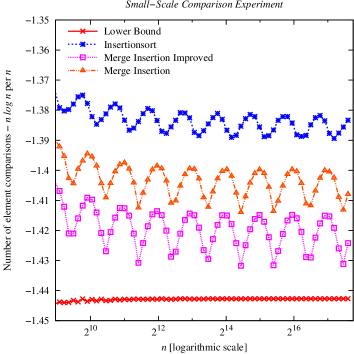
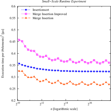
Figure 3: Comparison of MergeInsertion, its improved variant and Insertionsort. For the number of comparisons $n\log n+\kappa n$ the value of $\kappa$ is displayed.

The second part of our experiments (shown in Fig. 4) consists of the comparison of QuickMergesort (with base cases of constant and growing size) and QuickWeakHeapsort with state-of-the-art algorithms as STL-Introsort (i. e., Quicksort), STL-stable-sort (an implementation of Mergesort) and Quicksort with median of $\sqrt{n}$ elements for pivot selection. For QuickMergesort with base cases, the improved variant of MergeInsertion is used to sort subarrays of size up to $40\log_{10}n$. For the normal QuickMergesort we used base cases of size $\leq 9$. We also implemented QuickMergesort with median of three for pivot selection, which turns out to be practically efficient, although it needs slightly more comparisons than QuickMergesort with median of $\sqrt{n}$. However, since also the larger half of the partitioned array can be sorted with Mergesort, the difference to the median of $\sqrt{n}$ version is not as big as in QuickHeapsort [2]. As suggested by the theory, we see that our improved QuickMergesort implementation with growing size base cases MergeInsertion yields a result for the constant in the linear term that is in the range of $[-1.41,-1.40]$ – close to the lower bound. However, for the running time, normal QuickMergesort as well as the STL-variants Introsort (std::sort) and BottomUpMergesort (std::stable_sort) are slightly better. With about 15% the time gap, however, is not overly big, and may be bridged with additional efforts like skewed pivots and refined partitioning. Also, if comparisons are more expensive, QuickMergesort should perform significantly faster than Introsort.

   

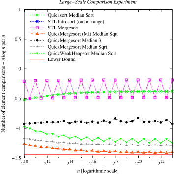
Figure 4: Comparison of QuickMergesort (with base cases of constant and growing size) and QuickWeakHeapsort with other sorting algorithms; (MI) is short for including growing size base cases derived from MergeInsertion. For the number of comparisons $n\log n+\kappa n$ the value of $\kappa$ is displayed.

7 Concluding Remarks

Sorting $n$ elements remains a fascinating topic for computer scientists both from a theoretical and from a practical point of view. With QuickXsort we have described a procedure how to convert an external sorting algorithm into an internal one introducing only $o(n)$ additional comparisons on average. We presented QuickWeakHeapsort and QuickMergesort as two examples for this construction. QuickMergesort is close to the lower bound for the average number of comparisons and at the same time is practically efficient, even when the comparisons are fast.

Using MergeInsertion to sort base cases of growing size for QuickMergesort, we derive an an upper bound of $n\log n-1.3999n+o(n)$ comparisons for the average case. As far as we know a better result has not been published before. Our experimental results validate the theoretical considerations and indicate that the factor $-1.43$ can be beaten. Of course, there is still room in closing the gap to the lower bound of $n\log n-1.44n+\mathcal{O}(\log n)$ comparisons.

Appendix A Pseudocode

procedure: $\mathit{construct}$($s$: array of elements, $r$: array of $n$ bits, $m$ bound)

for $k=m-1\ \mbox{\bf downto}\ 1$ 

       if $i+1=k$ then

             if $\textit{even}(k)$ then

                   $\mbox{$\mathit{join}$}(\mbox{$\mathit{d}$\mbox{\rm-}$\mathit{ancestor}$}(i),i)$

                  

            $k\leftarrow\lfloor k/2\rfloor$

            

      else

             $\mbox{$\mathit{join}$}(\mbox{$\mathit{d}$\mbox{\rm-}$\mathit{ancestor}$}(i),i)$

            

procedure: $\mathit{d}$-$\mathit{ancestor}$($j$: index)

while $(j\mbox{ \emph{{bitand}} }1)=r_{\lfloor j/2\rfloor}$ 

       $j\leftarrow\lfloor j/2\rfloor$

      

return $\lfloor j/2\rfloor$

procedure: $\mathit{join}$($i,j$: indices)

if $s_{j}<s_{i}$ then

       $\mbox{\em swap}(s_{i},s_{j})$

       $r_{j}\leftarrow 1-r_{j}$

      

procedure: $\mathit{d}$-$\mathit{child}$($i,j$: indices)

$x\leftarrow\mathit{secondchild}(i)$

while $\mathit{firstchild}(x)<j$ 

       $x\leftarrow\mathit{firstchild}(x)$

      

return $x$

Algorithm 2 Constructing a weak heap for MergeInsertion.

procedure: $\mathit{binary}$-$\mathit{insert}$( $s$: array of $n$ elements, $\phi$: array of $n$ integers, $r$: array of $n$ bits, $f,d,t$ integers)

for $j=t\ \mbox{\bf downto}\ f+d+1$ 

       $\textit{swap}(\phi_{j-1},\phi_{j})$

      

$l\leftarrow f$

$r\leftarrow f+d$

while $l<r$ 

       $m\leftarrow(l+r)/2$

       if $s_{\phi_{f+d}}>s_{\phi_{m}}$ then

             $l\leftarrow m+1$

            

      else

             $r\leftarrow m$

            

for $j=f+d\ \mbox{\bf downto}\ l$ 

       $\textit{swap}(\phi_{j-1},\phi_{j})$

      

Algorithm 3 Binary insertion of elements in MergeInsertion algorithm.

procedure: $\mathit{mergeinsertionrecursive}$( $s$: array of $n$ elements, $\phi$: array of $n$ integers, $r$: array of $n$ bits )

if $k>2$ then

       $\mathit{mergeinsertionrecursive}$$(k\ \mathit{div}\ 2)$

       $\mathit{merge}$$(k)$

      

procedure: $\mathit{mergeinsertion}$( $s$: array of $n$ elements, $\phi$: array of $n$ integers, $r$: array of $n$ bits )

$\mathit{construct}$$(n)$

$\mathit{mergeinsertionrecursive}$$(n)$

Algorithm 4 Main routine and recursive call for MergeInsertion algorithm.

References

• [1] D.Β Cantone and G.Β Cinotti. QuickHeapsort, an efficient mix of classical sorting algorithms. Theoretical Comput. Sci., 285(1):25–42, 2002.
• [2] V.Β Diekert and A.Β Weiß. Quickheapsort: Modifications and improved analysis. In A.Β A. Bulatov and A.Β M. Shur, editors, CSR, volume 7913 of Lecture Notes in Computer Science, pages 24–35. Springer, 2013.
• [3] R.Β D. Dutton. Weak-heap sort. BIT, 33(3):372–381, 1993.
• [4] S.Β Edelkamp and P.Β Stiegeler. Implementing HEAPSORT with $n\log n-0.9n$ and QUICKSORT with $n\log n+0.2n$ comparisons. ACM Journal of Experimental Algorithmics, 10(5), 2002.
• [5] S.Β Edelkamp and I.Β Wegener. On the performance of Weak-Heapsort. In 17th Annual Symposium on Theoretical Aspects of Computer Science, volume 1770, pages 254–266. Springer-Verlag, 2000.
• [6] A.Β Elmasry, J.Β Katajainen, and M.Β Stenmark. Branch mispredictions don’t affect mergesort. In SEA, pages 160–171, 2012.
• [7] J.Β Ford, LesterΒ R. and S.Β M. Johnson. A tournament problem. The American Mathematical Monthly, 66(5):pp. 387–389, 1959.
• [8] J.Β Katajainen. The Ultimate Heapsort. In CATS, pages 87–96, 1998.
• [9] J.Β Katajainen, T.Β Pasanen, and J.Β Teuhola. Practical in-place mergesort. Nord. J. Comput., 3(1):27–40, 1996.
• [10] D.Β E. Knuth. Sorting and Searching, volumeΒ 3 of The Art of Computer Programming. Addison Wesley Longman, 2nd edition, 1998.
• [11] C.Β MartΓ­nez and S.Β Roura. Optimal Sampling Strategies in Quicksort and Quickselect. SIAM J. Comput., 31(3):683–705, 2001.
• [12] K.Β Reinhardt. Sorting in-place with a worst case complexity of $n\log n-1.3n+o(\log n)$ comparisons and $\epsilon n\log n+o(1)$ transports. In ISAAC, pages 489–498, 1992.
• [13] I.Β Wegener. Bottom-up-Heapsort, a new variant of Heapsort beating, on an average, Quicksort (if $n$ is not very small). Theoretical Comput. Sci., 118:81–98, 1993.