The Astrophysical Multipurpose Software Environment

We present the open source Astrophysical Multi-purpose Software Environment (AMUSE, www.amusecode.org), a component library for performing astrophysical simulations involving different physical domains and scales. It couples existing codes within a Python framework based on a communication layer using MPI. The interfaces are standardized for each domain and their implementation based on MPI guarantees that the whole framework is well-suited for distributed computation. It includes facilities for unit handling and data storage. Currently it includes codes for gravitational dynamics, stellar evolution, hydrodynamics and radiative transfer. Within each domain the interfaces to the codes are as similar as possible. We describe the design and implementation of AMUSE, as well as the main components and community codes currently supported and we discuss the code interactions facilitated by the framework. Additionally, we demonstrate how AMUSE can be used to resolve complex astrophysical problems by presenting example applications.

1 Introduction

Astrophysical simulation has become an indispensable tool to understand the formation and evolution of astrophysical systems. Problems ranging from planet formation to stellar evolution and from the formation of galaxies to structure formation in the universe have benefited from the development of sophisticated codes that can simulate the physics involved. The development of ever faster computer hardware, as ‘mandated’ by Moore’s law, has increased the computational power available enormously, and this trend has been reinforced by the emergence of Graphic Processing Units as general purpose computer engines precise enough for scientific applications. All this has meant that codes are able to handle large realistic simulations and generate enormous amounts of data.

However, most of the computer codes that are used have been developed with a particular problem in mind, and may not be immediately usable outside the domain of that application. For example, an N-body code may solve the gravitational dynamics of hundreds of thousand of stars, but may not include algorithms for stellar evolution or the dynamics of the gas between the stars. The development of the latter needs a whole different set of expertise that developers of the former may not have. This presents a barrier as the trend is to move beyond solutions to idealized problems to more realistic scenarios that take into account more complex physical interactions. This is not restricted to astrophysics: fields as diverse as molecular dynamics, aerospace engineering, climate and earth system modelling are experiencing a similar trend towards multiphysics simulation (Groen et al. 2012).

Within astrophysics, different ways of combining physical solvers are being pursued: examples are collaborations on large monolithic codes such as Flash  (Fryxell et al. 2000) or GADGET (Springel et al. 2001; Springel 2005), or the aggregation of codes in heterogeneous packages, e.g. NEMO (Teuben 1995). These approaches are limited by the effort needed to assemble and maintain evolving software packages (for monolithic codes) or by the lack of integration of their component software base (in the case of code packages). More recently the MUSE (Portegies Zwart et al. 2009, 2013) framework was developed to overcome these problems by binding existing codes into a modern and flexible scripting language.

Figure 1: Design of the AMUSE interface. This diagram represents the way in which a community code (“code”) is accessed from the AMUSE framework. The code has a thin layer of interface functions in its native language which communicate through an MPI message channel with the Python host process. On the Python side the user script (“AMUSE simulation script”) only accesses generic calls (“setup,” “evolve” etc.) to a high level interface. This high level interface calls the low level interface functions, hiding details about units and the code implementation. The communication through the MPI channel does not interfere with the code’s own parallelization because the latter has its own MPI_WORLD_COMM context.

AMUSE is an astrophysical implementation of the general principles of MUSE (Portegies Zwart et al. 2013). It presents a coherent interface and simplified access to astrophysical codes allowing for multi-physics simulations. The main characteristics of MUSE that make this possible are:

• physical coupling: by defining physically based interfaces to the modules, AMUSE allows tight coupling between them,

• consistency over domains: AMUSE has consistent data handling and consistent interfaces over different domains,

• unit module: AMUSE aims to be transparent with regard to the physical units employed by the different simulation codes,

• IO facilities: AMUSE includes file IO and converters for legacy formats. Code specific input and output routines are bypassed,

• error handling: codes can detect that a system evolves outside their domain of applicability, and can alert the framework to this fact (The capabilities of AMUSE handling code crashes - another MUSE requirement - is limited at the moment),

• multiple domains: MUSE does not define the actual application domain. The current capabilities of AMUSE are focused on four domains of astrophysics: gravitational dynamics, stellar evolution, hydrodynamics and radiative transfer.

In section 2 we present a technical overview of the design and architecture of AMUSE. The astrophysical domains and included codes are presented in section 3. The use of AMUSE for multi-physics astrophysical simulations is described in section 4. Applications and ongoing research are presented in section  5. We discuss the performance and testing aspects and some of the present limitations of AMUSE in section 6.

2 Design and Architecture

Building multiphysics simulation codes becomes increasingly complex with each new physical ingredient that is added. Many monolithic codes grow extending the base solver with additional physics. Even when this is successful, one is presented with the prospect of duplicating much of this work when a different solver or method is added, a situation that often arises when a slightly different regime is accessed than originally envisaged or when results need to be verified with a different method.

In order to limit the complexity we need to compartmentalize the codes. The fundamental idea of AMUSE is the abstraction of the functionality of simulation codes into physically motivated interfaces that hide their complexity and numerical implementation. AMUSE presents the user with optimized building blocks that can be combined into applications for numerical experiments. This means that the requirement of the high level interactions is not so much performance but one of algorithmic flexibility and ease of programming, and thus the use of a modern interpreted scripting language with object oriented features suggests itself. For this reason we have chosen to implement AMUSE in Python. In addition, Python has a large user and developer base, and many libraries are available. Amongst these are libraries for scientific computation, data analysis and visualization.

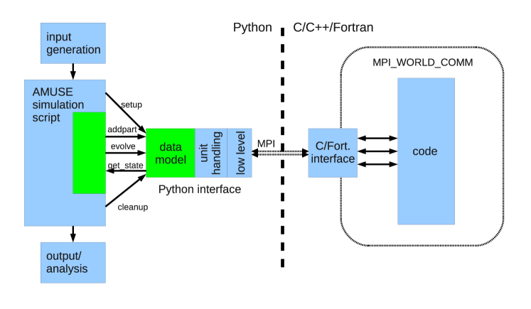
An AMUSE application consists roughly speaking of a user script, an interface layer and the community code base (Portegies Zwart et al. 2013, fig 1) . The user script is constructed by the user and specifies the initial data and the simulation codes to use. It may finish with analysis or plotting functions, in addition to writing simulation data to file. The setup and communication with the community code is handled by the interface layer, which consists of a communication interface with the community code as well as unit handling facilities and an abstract data model.

2.1 Remote function interface

(1) gravity=PhiGRAPE()
(2) gravity=PhiGRAPE(number_of_workers=32)
(3) gravity=PhiGRAPE(mode="GPU")
(4) gravity=PhiGRAPE(channel_type="estep",hostname="remote.host.name")

Figure 2: Starting a community code interface. (1) simple local startup, (2) startup of an MPI parallel worker with 32 worker processes, (3) startup of the community code with GPU support, (4) remote startup of worker.

The interface to a community code provides the equivalent functionality of importing the code as a shared object library. The default implementation in AMUSE is a remote function call protocol based on MPI. A community code is started by the straightforward instantiation of an interface object (fig. 2) transparent to this. Python provides the possibility of linking directly Fortran or C/C++ codes, however we found that a remote protocol provides two important benefits: 1) built-in parallelism 2) separation of memory space and thread safety. The choice for an intrinsically parallel interface is much preferable over an approach where parallelism is added a posteriori, because unless great care is taken in the design, features can creep in that preclude easy parallelization later on. The second benefit comes as a bonus: during early development we found that many legacy simulation codes make use of global storage that makes it either impossible or unwieldy to instantiate multiple copies of the same code - using MPI interfaces means that the codes run as separate executables, and thus this problem cannot occur. An additional advantage of the interface design is that the MPI protocol can be easily replaced by a different method, two of which are available: a channel based on sockets and one based on the eSTeP library for distributed computing. The sockets channel is currently mainly useful for cases were all the component processes are to be run on one machine. As its name implies it is based on standard TCP/IP sockets. The eSTeP channel is described below.

In practice the interface works as follows: when an instance of an imported simulation code is made, an MPI process is spawned as a separate process somewhere in the MPI cluster environment. This process consists of a simple event loop that waits for a message from the python side, executes the subroutines on the basis of the message ID and any additional data that may follow the initial MPI message, and sends the results back (see also Portegies Zwart et al. 2013). The messages from the python script may instruct the code to perform a calculation (like evolving for a specified amount of time), or may be a request to send or receive data. Calls can be executed synchronously (with the python script waiting for the code to finish) or asynchronously. The simulation code itself will continue executing the event loop, maintaining its memory state, until instructed to stop.

The benefit of using MPI must be weighed against the disadvantages, of which the two most important are: 1) it is more involved to construct an MPI interface and 2) there is no shared memory space, and thus also no direct access to simulation data. However, linking legacy C or Fortran codes (using SWIG or f2py) is actually not straightforward either and this concern is further alleviated by automating much of the interface construction (in AMUSE the source code for the main program on the client side is generated by a Python script and all the actual communication code is hidden). This means that the codes of the interfaces actually become more similar for codes of different target languages. The second issue is potentially more serious: communication using MPI is less direct than a memory reference. As a consequence the interfaces must be carefully designed to ensure all necessary information for a given physical domain can be retrieved. Additionally, the communication requirements between processes must not be too demanding. Where this is not the case (e.g. when a strong algorithmic coupling is necessary) a different approach may be more appropriate.

An obvious additional concern is the correct execution of MPI parallel simulation codes: the communication with the python host must not interfere with the communication specified in the code. This is guaranteed with the recursive parallelism mechanism in MPI-2. The spawned processes share a standard MPI_WORLD_COMM context, which ensures that an interface can be build around an existing MPI code with minimal adaptation (fig. 1). In practice, for the implementation of the interface for an MPI code one has to reckon with similar issues as for the stand-alone MPI application. The socket and eSTeP channels also accomodate MPI parallel processes.

2.1.1 Distributed Computing

Current computing resources available to researchers are more varied than simple workstations: clusters, clouds, grids, desktop grids, supercomputers and mobile devices complement stand-alone workstations, and in practice one may want to take advantage of this ecosystem, which has been termed Jungle computing (Seinstra et al. 2011), to quickly scale up calculations beyond local computing resources.

To run in a Jungle computing environment the eSTeP channel is available in AMUSE (Drost et al. 2012). Instead of using MPI this channel connects with the eSTeP daemon to start and communicate with remote workers. This daemon is aware of local and remote resources and the middleware over which they communicate (e.g. SSH). The daemon is started locally before running any remote code, but it can be re-used for different simulation runs. The eSTeP software is written in Java. Once the daemon is running, and a simulation requests a worker to be started, the daemon uses a deployment library to start the worker on a remote machine, executing the necessary authorization, queueing or scheduling. Because AMUSE contains large portions of C, C++, and Fortran, and requires a large number of libraries, it is not copied automatically, but it is assumed to be installed on the remote machine. A binary release is available for a variety of resources, such as clouds, that employ virtualization. With these modifications, AMUSE is capable of starting remote workers on any resource the user has access to, without much effort required from the user. In short, to use the distributed version of AMUSE one must (1) ensure that AMUSE is installed on all machines and (2) specify for each resource used some basic information, such as hostname and type of middleware, in a configuration file. Once (1) and (2) are done, any AMUSE script can be distributed by simply adding properties to each worker instantiation in the script, specifying the channel used, as well as the name of the resource, and the number of nodes required for this worker (see figure 2).

2.1.2 AMUSE Job server

Python scripts can also be interfaced with AMUSE using either the MPI or sockets/eSTeP channel. One unintended but pleasant consequence of this is that it is very easy to run an AMUSE script remotely, and to build a framework to farm out AMUSE scripts over the local network machines - or using eSTeP over any machines connected to the internet - in order to marshall computing resources to quickly do e.g. a survey of runs. AMUSE includes a module, the JobServer, to expedite this.

2.2 Unit conversion

(1) m= 1 | units.MSun
(2) m= [ 1., 2.] | units.MSun
(3) def escape_velocity(mass,distance,G=constants.G):
      return sqrt(G*mass/distance)
    v=escape_velocity(m, 1.| units.AU)
(4) dt=1.| units.hour
    (v*dt).in_(units.km)

(1) converter=nbody_system.nbody_to_si( 1. | units.MSun, 1.| units.AU )
(2) converter.to_si(1. | nbody_system.time)
(3) converter.to_nbody(1. | units.kms)

Figure 3: The AMUSE units module. The upper panel illustrates the use of the unit algebra module. (1) definition of a scalar quantity using the $|$ operator, (2) definition of a vector quantity (3) use of units in functions and (4) conversion of units. Lower panel illustrates the use of a converter between N-body units and SI. (1) defines a converter from units with G=1 (implicit), ${\rm\thinspace M_{\odot}}=1$ and AU=1 to SI units, (2) conversion to SI units, (3) conversion from SI units.

Keeping track of different systems of units and the various conversion factors when using different codes quickly becomes tedious and prone to errors. In order to simplify the handling of units, a unit algebra module is included in AMUSE (figure 3). This module wraps standard Python numeric types or Numpy arrays, such that the resulting quantities (i.e. a numeric value together with a unit) can transparently be used as numeric types (see the function definition example in figure 3). Even high level algorithms, like e.g. ODE solvers, typically do not need extensive modification to work with AMUSE quantities.

AMUSE enforces the use of units in the high level interfaces. The specification of the unit dimensions of the interface functions needs to be done only once, at the time the interface to the code is programmed. Using the unit-aware interfaces, any data that is exchanged within modules will be automatically converted without additional user input, or - if the units are not commensurate - an error is generated.

Often codes will use a system of units that is underspecified, e.g. most N-body codes use a system of units where $G=1$. Within AMUSE these codes can be provided with data in this system of units (N-body units) or, using a helper class specifying the scaling, in physical units. Figure  3 shows an example of such a converter. Converters are often necessary when a code that uses scale-free units is coupled to another code which uses a definite unit scale (e.g. a gravitational dynamics code coupled to a stellar evolution code, where the latter has definite input mass scales).

2.3 Data model

(1) cluster=new_plummer_model(100)
(2) cluster.x+=10| units.kpc
(3) cluster[0:5].velocity=0. | units.kms
(4) galaxy.add_particles( cluster )
(5) gravity.particles.add_particles( cluster )
(6) channel=gravity.particles.new_channel_to( cluster )
(7) channel.copy_attributes( ["position","velocity"] )

Figure 4: Example usage of high level particles sets. (1) initialize a set, (2) shift particle positions, (3) indexing of particle sets, (4) joining two particle sets, (5) sending particle data to a code, (6) definition of an explicit channel from in-code storage to a particle set in memory (7) update of particle attributes over the channel. Similar data structures are available for grids as needed for e.g. grid hydrodynamic solvers.

The low level interface works with ordinary arrays for input and output. While this is simple and closely matches the underlying C or Fortran interface, its direct use entails a lot of duplicated bookkeeping code in the user script. Therefore in order to simplify work with the code, a data model is added to AMUSE based on the construction of particle sets, see figure 4. Here a particle is a an abstract object with different attributes (eg. mass, position etc) and a unique ID. The data model and the unit interface are combined in a wrapper to the plain (low level) interface. The particle sets also include support code for a set of utility functions commonly needed (e.g. calculation of center of mass, kinetic energy, etc).

Particle sets store their data in Python memory space or reference the particle data in the memory space of the community code. A particle set with storage in the community code copies the data from the code transparently upon access. The data of a memory set can be synchronized explicitly by defining a channel between the memory particle set and the code particle set ((6) and (7) in figure 4). Hence, data is only transferred from a code by accessing the attributes of its in-code particle set, or by a copy operation of a channel between such a set and another set.

Subsets can be defined on particle sets without additional storage and new sets can be constructed using simple operations (addition, subtraction). The same methods of the parent set are available for the subsets (but only affecting the subset).

A similar datastructure is defined for grids. A Grid set consists of a description of the grid properties and a set of grid points with attributes.

2.4 State Model

Figure 5: State model of gravitational dynamics codes. The diagram gives the state that a gravitational dynamics code can be in. Transitions can be effected explicitly (by calling the corresponding function, e.g. initialize_code from ‘start’ to ‘init,’ or implicitly (e.g. calling get_position to get the position of a particle is only allowed in the ‘run’ state - the framework will call the necessary functions to get in that state, which will be a difference sequence of functions depending on the starting state).

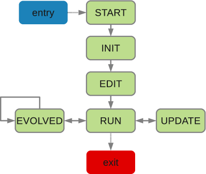
When combining codes that use very different algorithms to represent the same physics one quickly runs into the problem that different codes have different work-flows. For example, the gravitational dynamics interface defines methods to add and remove particles and the calculation of gravitational forces obviously needs to track these changes. However, for, for example, a gravitational Barnes-Hut type tree code the data structure of the tree has to be updated before the new gravitational forces can be calculated. Such a tree update is an expensive operation. It is undesirable to add explicit tree update functions to the gravitational interface, as this functionality only makes sense for tree codes. One way to solve this would be program the interface code of the add-particle method of a tree code to update the tree each time, but this would be highly inefficient if a large group of particles is added to the code. The more efficient approach in this case is to flag the state of the code and do a tree update once all particle transactions have been completed. The only problem with this is that it is error prone if under control of the user. We have added facilities to AMUSE to keep track of the state a code is in, and to change state automatically if an operation is requested that is not allowed in the current state and to return an error if the state transition is not allowed. For the example above, this means that in the user script the addition and removal of particles is the same for all gravitational codes, but that in the case of a tree code an automatic call is made to the tree update routine once the user script proceeds to request, for example, a gravitational force.

The state model is flexible: states can be added and removed as required, but in practice similar codes share similar state models. e.g. all the gravitational dynamics codes included in AMUSE conform to the state model with six states shown in fig. 5.

2.5 Object oriented interfaces

 gravity=BHTree()
 gravity.initialize_code()
 gravity.set_eps2( 0.00155 )
 gravity.commit_parameters()
 for i in range(n):
   gravity.add_particle(mass[i],radius[i],
           x[i],y[i],z[i],vx[i],vy[i],vz[i])
 gravity.commit_particles()
 gravity.evolve_model( 6.707 )

 gravity=BHTree()
 gravity.parameters.epsilon_squared=(1 | units.pc)**2
 gravity.particles.add_particles(stars)
 gravity.evolve_model( 100. | units.Myr)

Figure 6: Low level vs high level object oriented interface. The upper panel shows the schematic calling sequence for the low level interface of a gravity module, The lower panel shows the equivalent using the high level interface.

The object oriented, or high level, interfaces are the recommended way of interacting with the community codes. They consist of the low-level MPI interface to a code, with the unit handling, data model and state model on top of it. At this level the interactions with the code are uniform across different codes and the details of the code are hidden as much as possible. The difference in calling sequence is illustrated in figure  6. A lot of the bookkeeping (arrays/ unit conversion) is absent in the high level interface formulation. This makes the high level interface much easier to work with and less prone to errors: the user does not need to know what internal units the code is using, and does not need to remember the calling sequence nor the specific argument order of calls.

2.6 IO conversion

The community codes that are included into AMUSE normally contain subroutines to read in and write simulation data. This functionality is not used within AMUSE. Instead, all simulation data is written and read from within the AMUSE script (if tabulated data sets are needed by a community code, e.g. opacity tables, these are read by the code in the course of the initialization process). AMUSE includes a default output format based on hdf5 that writes out all data pertaining to a data set. In order to simplify import and export of data, AMUSE contains a framework for generic I/O to and from different file formats. A number of common file formats are implemented (Starlab, Gadget, Nemo), as well as generic table format file readers.

2.7 Initial conditions and data analysis

Although not a main objective for AMUSE, some provisions are made to facilitate the generation or import of initial conditions and the analysis of data generated by a simulation. A number of N-body specific analysis tools are available by default (such as energy diagnostics, lagrangian radii, binary detection).

The generation of initial conditions for astrophysical simulations is often non-trivial, with specialized initial condition codes being used to construct initial density distributions or stellar structure models. As such, a limited selection of common initial condition generators is included in AMUSE. A number of the more common N-body particle generators (Plummer and King models), a selection of basic grid generators (random, regular cubic grid and regular body centered cubic grids), useful for the generation of SPH initial conditions and zero age main sequence (ZAMS) stellar evolution model generators are available. This allows simple tests and experiments to be quickly developed. A number of more advanced initial condition generators, such as the GalactICS code for galaxy models (Widrow et al. 2008) or the FractalCluster code  (Goodwin & Whitworth 2004), are also interfaced.

After a simulation, the generated data needs to be analyzed. A limited collection of analysis tools is distributed with AMUSE. Python has good numerical and plotting libraries, such as Numpy and Matplotlib, available and data analysis can be easily incorporated into the AMUSE workflow. The nature of the data sets often means that visualization can be very helpful for the interpretation. Blender is python scriptable and can be used to visualize 3D data sets. In addition, simple OpenGL utilities can be coupled to the community codes to inspect the simulation data at runtime, especially useful in the development and debugging stage.

2.8 Importing codes

Bringing a new code into the framework involves a number of steps. The complete procedure (along with examples) is described in detail in the documentation section of the source distribution and the project website. Here we outline the procedure.

To import a community code the code one first creates a directory in the AMUSE community code base directory with the name of the module. The original source tree is imported in a subdirectory (by convention named ‘ src’). The top-level directory also contains the Python side of the interface (‘interface.py’), the interface in the native language of the code (e.g. ‘interface.c’) and a file for the build system (‘Makefile’).

The Python interface (the file interface.py) typically defines two classes which define the low-level interface functions (as much as possible by inheritance from one of the base interface classes) and the high level interface. The low level interface then contains the function definitions of the calls which are redirected through the MPI communications channel (see section 2.1) to the corresponding call defined in the native interface file (interface.c). The high level interface defines the units of the arguments of the function calls where appropriate (see section 2.2). In addition it specifies the parameters of the code, the state model (section 2.4) and the mapping of the object oriented data types to the corresponding low-level calls. By default the data of the simulation is maintained in the community code’s memory (and accessed transparently as described in section 2.3).

The modifications to the code itself (in ‘src’) that are necessary fall in the following loosely defined categories: 1) In the most favourable case no modifications to the community code’s source base are necessary and only the Python and native interfaces need to be added. For modern and modular codes this is often the case. 2) In addition to the interface code, it may be necessary to add a small library of helper functions, either to provide some secondary functionality that was not part of the community code (e.g. a gravity code may not have had functionality to change the number of particles in memory) or to reorganize previously existing code (e.g. the initialization, read-in and simulation loop might have been written in a single main program, where in AMUSE they need to be separated). 3) or a code may need significant source code changes to implement functionality that was not present but required for the AMUSE interface (e.g. externally imposed boundary conditions for grid hydrodynamics).

It is clear that the actual effort needed to interface a community code increases as succesively more changes are necessary. Apart from this, it also becomes more difficult from the viewpoint of code maintenance: when a new version of a community code is brought into AMUSE, case 1) above may necessitate no additional steps beyond copying the updated version, while in case 3), the adaptations to the community code need to be carefully ported over.

3 Component modules

The target domains for the initial release of AMUSE were gravitational dynamics, stellar evolution, hydrodynamics (grid and particle based) and radiative transfer. For a given physical domain, the community codes that are included in AMUSE share a similar interface that is tailored to its domain. An overview of all the codes that are included in the current release (version 7.1) is given in Table 1. This selection of community codes is the result of a somewhat organic growth process where some codes were selected early on in the development of AMUSE to demonstrate proof of principle, others were contributed by their respective authors as a result of collaborations. We have taken care though that each domain is represented by at least 2 different codes, as this is the minimum to be able to conduct cross verification of simulations (cf. “Noah’s Ark” objective, Portegies Zwart et al. 2009). AMUSE can be extended by including other codes and domains, which can then be contributed to the AMUSE repository.

code	language	short description	main reference
Hermite0	C++	Hermite N-body	Hut et al. (1995)
PhiGRAPE	Fortran, MPI/GPU	Hermite N-body	Harfst et al. (2007)
ph4	C++, MPI/GPU	Hermite N-body	McMillan, in prep.
BHTree	C++	Barnes-Hut treecode	Barnes & Hut (1986)
Octgrav	C++, CUDA	Barnes-Hut treecode	Gaburov et al. (2010)
Bonsai	C++, CUDA	Barnes-Hut treecode	Bédorf et al. (2012)
Twobody	Python	Kepler solver	Bate et al. (1971)
Huayno	C, OpenMP/OpenCL	Hamiltonian splitting	Pelupessy et al. (2012)
SmallN	C++	regularized solver	Portegies Zwart et al. (1999)
Mercury	Fortran	symplectic planetary integrator	Chambers (1999)
Mikkola	Fortran	relativistic regularization	Mikkola & Merritt (2008)
MI6	C++, MPI/GPU	Hermite with Post-Newtonian terms	Iwasawa et al. (2011)
Pikachu	C++, CUDA	Hybrid Barnes-Hut/Hermite	Iwasawa et al., in prep.
Brutus	C++, MPI	arbitrary precision Bulirsch-Stoer	Boekholt & Portegies Zwart, in prep.
HiGPUs	C++, CUDA	Hermite N-body	Capuzzo-Dolcetta et al. (2013)
Tupan	Python, OpenCL	Symplectic N-body, Post-Newtonian	Ferrari, in prep.
MMC	Fortran	Monte-Carlo gravitational dynamics	Giersz (2006)
SSE	Fortran	stellar evolution fits	Hurley et al. (2000)
Evtwin	Fortran	Henyey stellar evolution	Glebbeek et al. (2008)
MESA	Fortran, OpenMP	Henyey stellar evolution	Paxton et al. (2011)
BSE	Fortran	binary evolution	Hurley et al. (2000)
SeBa	C++	stellar and binary evolution	Portegies Zwart et al. (2001)
Fi	Fortran, OpenMP	TreeSPH	Pelupessy (2005)
Gadget-2	C, MPI	TreeSPH	Springel (2005)
Capreole	Fortran, MPI	Finite volume grid hydrodynamics	Mellema et al. (1991)
Athena3D	C, MPI	Finite volume grid hydrodynamics	Stone et al. (2008)
MPIAMRVAC	Fortran, MPI	AMR code for conservation laws	Keppens et al. (2012)
Simplex	C++, MPI	Rad. transport on Delaunay grid	Paardekooper et al. (2010)
SPHRAY	Fortran	Monte Carlo on SPH particles	Altay et al. (2008)
Mocassin	Fortran	Monte Carlo, steady state	Ercolano et al. (2003)
MMAMS	C++	stellar mergers by entropy sorting	Gaburov et al. (2008)
Hop	C++	particle group finder	Eisenstein & Hut (1998)
FractalCluster	Fortran	Fractal cluster generator	Goodwin & Whitworth (2004)
Halogen	C	Halo distribution functions	Zemp et al. (2008)
GalactICS	C	Galaxy model generator	Widrow et al. (2008)

Table 1: Overview of community codes included in the public release of AMUSE. Table lists the name of the code, the language it is written in and the parallelization model, a short description and a reference to either the code paper or a description of the method.

3.1 Gravitational dynamics

The gravity codes included in AMUSE span most dynamic regimes except that support for large scale cosmological simulations is limited. Fully relativistic metric solvers are also not included at present. Hermite0, PhiGRAPE, ph4 and HiGPUs are direct N-body integrators with Hermite timestepping schemes, where the latter three are tooled to use hardware (GRAPE or GPU) accelerated force calculations. All are MPI parallelized. Huayno is a (semi-)symplectic integrator based on Hamiltonian splitting. BHTree, Octgrav and Bonsai are Barnes-Hut treecodes (Octree is partly GPU accelerated, Bonsai runs completely on the GPU). Twobody, SmallN and Mikkola are integrators that calculate the dynamics for small N systems using analytic solutions and regularization respectively (with relativistic corrections in the case of Mikkola). Such solvers are also potentially useful as components in compound gravity solvers where one of the other solvers is used for the general dynamics and close passages and binaries are handled by a small N solver (see section 4). Tupan is a symplectic integrator with post-newtonian correction terms. Mercury and MI6 are examples of a specialized class of gravitational integrators, geared towards long time evolution of systems dominated by a central object: planetary systems for Mercury, black hole dominated systems for MI6. Brutus and MMC represent two completely opposite approaches in a sense to solving gravitational dynamics: Brutus uses arbitrary precision arithmetic libraries to obtain converged solutions, while MMC uses Monte Carlo gravitational dynamics to solve globular cluster dynamics. Finally, the N-body/SPH codes included in AMUSE (Fi and Gadget) can also be used in mixed gravity/hydrodynamics or purely gravitational mode (see section  3.3). They also conform to the gravitational dynamics interface.

code	small N	intermediate N	large N	large N	centrally dominated	post-Newtonian
	(collisional)	(collisional)	(collisional)	(collisionless)
Hermite0	$+$	$+$	$\circ$	$\circ$	$\circ$	$-$
PhiGRAPE	$+$	$+$	$+$	$\circ$	$\circ$	$-$
ph4	$+$	$+$	$+$	$\circ$	$\circ$	$-$
BHTree	$-$	$-$	$-$	$+$	$-$	$-$
Octgrav	$-$	$-$	$-$	$+$	$-$	$-$
Bonsai	$-$	$-$	$-$	$+$	$-$	$-$
Twobody	N=2	$-$	$-$	$-$	$+$	$-$
Huayno	$+$	$+$	$+$	$\circ$	$\circ$	$-$
SmallN	$+$	$-$	$-$	$-$	$-$	$-$
Mercury	$-$	$-$	$-$	$-$	$+$	$-$
Mikkola	$+$	$-$	$-$	$-$	$-$	$+$
MI6	$+$	$+$	$+$	$-$	$+$	$+$
Pikachu	$+$	$+$	$+$	$+$	$-$	$-$
Brutus	$+$	$-$	$-$	$-$	$+$	$-$
HiGPUs	$-$	$+$	$+$	$\circ$	$-$	$-$
Tupan	$+$	$+$	$\circ$	$\circ$	$\circ$	$+$
MMC	$-$	$-$	$+$	$-$	$-$	$-$
Fi	$-$	$-$	$-$	$+$	$-$	$-$
Gadget2	$-$	$-$	$-$	$+$	$-$	$-$

Table 2: Overview of the suitability of gravitational dynamics solvers for different gravitational regimes. A $+$ indicates that a codes is well suited to a particular regime, a $-$ indicates that the code will fail or run very inefficiently, a $\circ$ indicates a limited capability; “small N” means a problem with a small number of bodies, N$\approx 2-100$, “intermediate N” means N$\approx 100-10^{4}$ , “large N” means N $\gtrsim 10^{4}$ , “collisionless” indicates gravitational dynamics with some form of softening, “collisional” means simulations without softening. “Centrally dominated” means problems were the dynamics is dominated by a massive central object, such as a solar system or cluster with a supermassive black hole. “Post-Newtonian” indicates whether the code includes post-Newtonian correction terms. Note this table does not address special requirements set by the timescales or the dynamic range of a problem, nor the choice of parameters that may affect the solutions.

The interface to the different gravitational dynamics codes is the same and changing the core integrator in a script is trivial. However, the gravitational dynamics integrators that are included in AMUSE are geared towards different types of problem: choosing a correct and efficient integrator for a particular problem is the responsibility of the AMUSE user, however table 2 gives a rough overview of the suitability of the various integrators in different regimes.

3.2 Stellar evolution

0: deeply or fully convective low mass main seq. star
1: main sequence star
2: hertzsprung gap
3: first giant branch
4: core helium burning
5: first asymptotic giant branch
6: second asymptotic giant branch
7: main sequence naked helium star
8: hertzsprung gap naked helium star
9: giant branch naked helium star
10: helium white dwarf
11: carbon/oxygen white dwarf
12: oxygen/neon white dwarf
13: neutron star
14: black hole
15: massless supernova
16: unknown stellar type
17: pre-main-sequence star

Figure 7: Stellar types used in AMUSE.

The stellar evolution codes currently included fall into two categories: table or parametrized fits based and Henyey-type solvers (1D evolution code). SSE implements simple heuristics and table look-up to determine approximate stellar evolution tracks. BSE and SeBa are the equivalent of SSE for binary system evolution. Evtwin and MESA are (Henyey-type) solvers for stellar evolution. They calculate the full internal evolution of a 1D model for a star Henyey et al. (1959, 1964); Eggleton (1971); Paxton et al. (2011). They share however the same basic interface as table based stellar evolution codes (with the details of the internal evolution hidden) and can be used interchangeably. In addition, for the full stellar evolution codes the internal (1D) structure of the stars can be accessed. The internal structure (basically radial profiles) can be used to construct 3D hydrodynamic models of stars (see section 4). During the evolution of a stellar model a stellar evolution code may encounter a phase where numerical instabilities are encounterd (e.g. during the Helium flash). Below we describe our strategy to handle this error condition.

3.2.1 Robust stellar evolution with fallback

Figure 8: Stellar evolution with SSE Fallback. Shown are evolutionary tracks calculated with EVTWIN (drawn lines), with SSE fallback (dashed lines) in case the full stellar evolution code could not progress. For this particular version of EVTWIN this happened at the Helium or Carbon flash. Stellar type labels are given in figure 7.

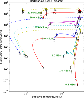
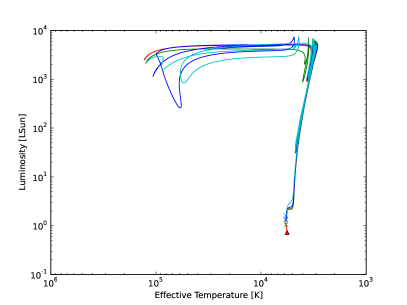
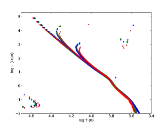
The typical use case of a stellar evolution code in AMUSE may be as a subcode in a larger script, for example when calculating the evolution of a star cluster with stellar collisions, where the collision cross section depends on the radii of the stars (and hence on its evolution). However, stellar evolution physics is considerably more complicated than gravitational dynamics in the sense that numerical instabilities may be encountered, which may slow down these codes tremendously or even require manual intervention. Within AMUSE we have the option to use a code based on lookup tables like SSE as a fallback code, since such codes will always find a solution. This pragmatic solution may be justified if the fallback option is only rarely needed. As an example we show the Herzpsrung-Russel diagram of a set of stars evolved using EVtwin, with SSE as a fallback option. The actual implementation of the fallback minimizes the $\chi^{2}$ error on the luminosity, radius and mass to find the closest matching SSE model at a given switchpoint.

3.3 Hydrodynamics

Figure 9: Kevin-Helmholtz test. Shown are the density distribution at $t=1$ for Athena (left panel), Capreole (middle panel) and MPIAMRVAC (right panel). Random velocities were seeded with an amplitude of $0.01c_{s}$

Figure 10: Cloud-shock test. Comparison of the results of the cloud-shock test (Agertz et al. 2007) for 3 grid hydrodynamic codes (each row showing results for respectively Athena, Capreole and MPIAMRVAC). Panels show slices through the 3D density distribution for times $t={0.25,1.,1.75,2.5}\times\tau_{\rm KH}$. The resolution for Athena and Capreole is 320x320x1280, for MPIAMRVAC it is 80x80x320 with 2 levels of refinement for the same effective resolution.

In hydrodynamics a distinction is made between two types of code: particle based codes and grid based codes. Particle based methods include for example Smooth Particle Hydrodynamics (SPH) codes. Grid based codes may be further subdivided into Eulerian and Langrangian (comoving) grid codes. AMUSE is limited at the moment to Eulerian grid solvers on regular Cartesian grids, which may be statically or dynamically refined.

Most current astrophysical SPH codes contain solvers for gravitational dynamics (using the  Hernquist & Katz (1989) TreeSPH scheme) and can evolve collisionless particles in addition to gas particles. Hence the interface to these codes define at least two different sets of particles, (particles and gas_particles). The interface of these codes contains a subset restricted to the particles that conforms to the specification of the gravitational dynamics interface. The hydrodynamic part of the interface is very similar to the gravitational part, adding hydrodynamic state variables (density, internal energy) to the gas particles.

The fundamental difference of the grid hydrodynamics interface with respect to the particle hydrodynamics and gravitational interfaces is that it contains functions to specify the grid properties and boundary conditions and that the complete grid must be initialized before use. A complication for the inclusion of grid hydrodynamics is that these codes typically are compiled for a specific problem setup, which entails picking different source files for e.g. different grids or boundary conditions. Within AMUSE, this is hidden from the user by choosing cartesian grids and limiting the options with respect to boundary conditions (simple inflow/outflow, reflecting and periodic). This can be extended as needed.

Presently two parallel TreeSPH codes, Fi and Gadget, are included. In addition the grid hydrocodes Capreole, Athena3D and MPIAMRVAC are included. Capreole is a finite volume eulerian grid code based on Roe’s Riemann solver (Mellema et al. 1991). Athena3D is a finite volume Eulerian grid code for hydrodynamics and magnetohydrodynamics using different Riemann solvers (limited support for magnetohydrodynamics is implemented in AMUSE) and allows for static mesh refinement. MPIAMRVAC is an MPI-parallelized Adaptive Mesh Refinement code for hyperbolic partial differential equations geared towards conservation laws. Within AMUSE the hydrodynamic solver of MPIAMRVAC is implemented, including full AMR support.

3.3.1 Hydrodynamic test cases

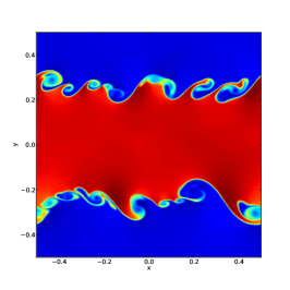
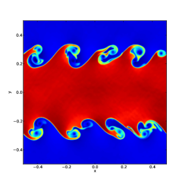
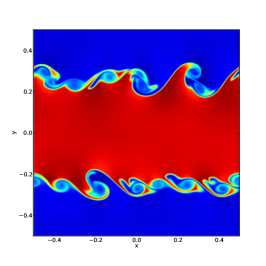
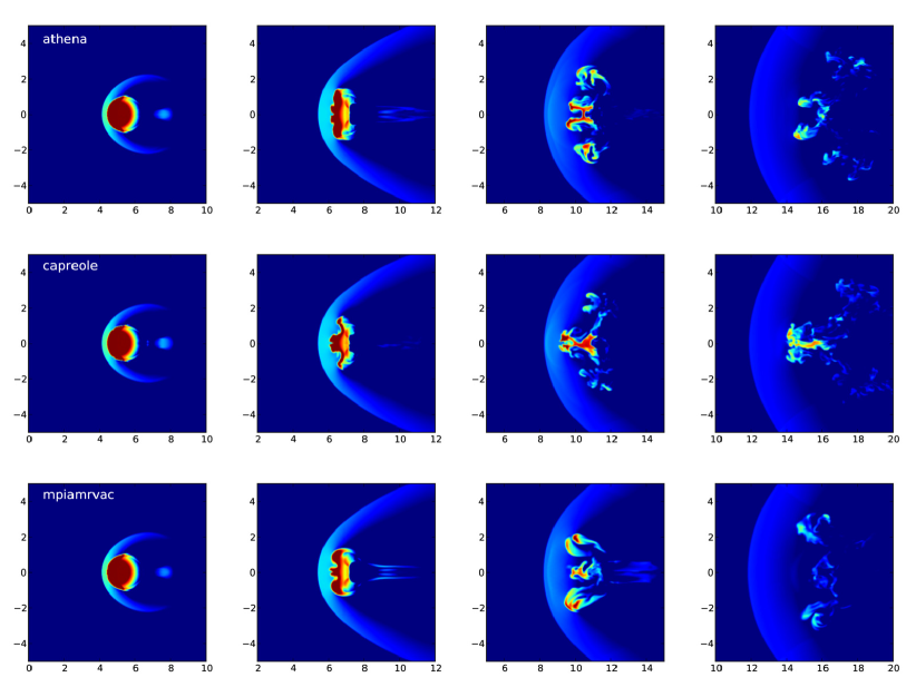
As an example we show the results of two common hydrodynamic tests using AMUSE, where the exact same script for different codes is used. The first test is the well known Kelvin-Helmholtz (KH) instability test (figure 9) which demonstrates the ability of the grid codes to model the KH instabilities. The second test, the cloud-shock test (Agertz et al. 2007), consists of a cloud compressed by a high mach number shock, representative of the shock-induced star formation process (figure  10).

3.4 Radiative transfer

Due to the high computational cost of radiative transfer caluclations, most radiative transfer codes are limited and optimized for a particular type of transport, e.g. photo-ionisation, dust or molecular line transfer. Within AMUSE the main focus is on photo-ionisation codes. They calculate the time dependent propagation of UV photons as well as the ionization and thermal balance of gas irradiated by hot stars or an AGN. Dust radiation transfer is in development. The latter is more important as a post-processing tool to generate realistic virtual observations or diagnostics.

AMUSE currently includes the photo-ionisation codes Simplex and SPHRay. SimpleX is based on the transport of radiation along the vertices of a Delaunay grid. It includes heating and cooling as well as H and He chemistry and contains optional treatment of diffuse recombination radiation. SPHRay is a Monte-Carlo photo-ionisation code which works on (SPH) particle distributions directly - it solves similar physics as SimpleX.

In addition, a proto-type interface for the Monte Carlo code Mocassin is available. Mocassin calculates a more extensive chemical network than SimpleX or SPHRay, albeit in the steady state approximation.

Figure 11: Conversion of a stellar evolution model to SPH and back. Left panel shows a $N=10^{5}$ SPH realization of a $1{\rm\thinspace M_{\odot}}$ MESA stellar evolution model at 5 Gyr. Right panel shows the HR diagram of the evolution of a $1{\rm\thinspace M_{\odot}}$ MESA model, as well as as the evolution of a MESA model derived from the SPH model, as well as two additional models which where converted at 8 and 10 Gyr of age. As can be seen the conversion at later evolutionary stages induces bigger deviations from normal evolution, probably because of the increased density contrasts (as the core becomes denser) at later times means that the particle distributions induce more mixing.

4 Compound solvers

Figure 12: Integration of an Oort cloud comet in a time-dependent galaxy potential. Upper panel shows the 3 eigenvalues of the tidal tensor extracted from a milky way galaxy simulation, the lower panel shows an integration of an Oort cloud comet subject to the corresponding tidal tensor, integrated using the Bridge integrator.

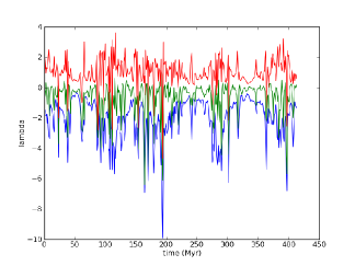
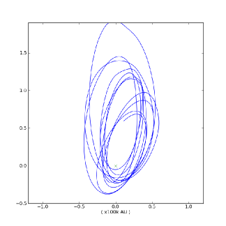
In addition to provide a unified interface to various types of codes, AMUSE has the objective of facilitating multiphysics simulations. For example, one would want to combine a gravitational dynamics code with a collision solver to construct a compound solver for gravitational dynamics that allows integration past a collision. Community codes can be combined within AMUSE such that the compound solver has a wider applicability than each by itself. The setup of AMUSE allows for this in a transparent manner, such that a combined solver has a similar interface as a plain code. The types of coupling AMUSE can be applied to fall roughly in the following categories (Portegies Zwart et al. 2013):

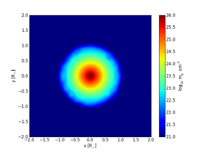
• input/ouput coupling: the loosest type of coupling occurs when the result of one code generates the initial conditions for another code. For example: a 3 dimensional SPH star model can be generated from a stellar evolution code, or vice versa (figure 11),

• one way coupling: one system interacts with another (sub)system , but this (sub)system does not couple back (or only very weakly) to the former. An example may be the stellar evolution of stars in a cluster, where the mass loss of the stars is important for the dynamics, but the dynamics of the cluster does not affect the stellar evolution (see section 4.1),

• hierarchical coupling: one or more systems are embedded in a parent system, which affects the evolution, but the subsystems do not affect the parent or each other. An example is the evolution of cometary orbits of the Oort cloud in a realistic galactic potential (figure 12),

• serial coupling: a system evolves through clearly separate regimes, such that different codes have to be applied in an interleaved way. An example may be a dense cluster where stellar collisions occur. In such a system, pure gravitational dynamics may be applied until the moment a collision between two stars is detected, at which point such a collision can be resolved using e.g. a full hydrodynamic code. After the hydrodynamic calculation the collision product is reinserted in the stellar dynamics code (see section 4.2),

• interaction coupling: this type of coupling occurs when there is neither a clear seperation in time nor spatially. An example may be the coupling between the ISM and stellar dynamics, where the gas dynamics must account for the combined potential of the gas and stars (see section 4.4),

• intrinsic coupling: this may occur where the physics of the problem necessitates a solver that encompasses both types of physics. An example may be magnetohydrodynamics, where the gas dynamics and the electrodynamics of the problem are so tightly coupled it makes little sense to seperate the two. In such a case an integrated solver can be included in AMUSE.

With the exception of the last type of coupling, these couplings can be implemented in AMUSE using single component solvers. To increase the flexibility in combining different solvers, the interface definitions contain functions to transfer physical quantities. For example, the gravity interface definition includes functions to sample the gravity force at any location and the hydrodynamic interface can return the hydrodynamic state vector at any point. In addition, the AMUSE interface contains a framework to detect when a simulation code evolves outside its domain of validity using stopping conditions. At least as important as being able to evolve the system in time, is the ability to actually detect when the calculation goes outside the regime where the solver is reliable. For gravity modules this may be for example a detection of close passages or collisions. For a hydrodynamics with self gravity this may be an instability criterion on density and internal energy (Whitworth 1998).

In the remainder of this section we elaborate on a number of examples to illustrate the coupling strategies that can be employed within AMUSE. We note that, while AMUSE facilitates these kinds of couplings, it remains the responsibility of the user to check the validity of the chosen coupling strategy in the regime of interest.

4.1 Cluster evolution with full stellar evolution

Stellar evolution affects the global evolution of a cluster of stars by dictating the mass loss of the stars. In the simplest approximation the stellar ejecta are assumed to escape instantaneously from the cluster. The only two codes needed to calculate this are then: a stellar evolution code to calculate the time dependent stellar mass loss, and a gravitational dynamics code to calculate the dynamics of the stars. The integration proceeds as follows: the gravitational dynamics code is advanced for a time $\Delta t$, at the end of this time the stellar evolution code is synchronized to the current simulation time and the stellar masses in the gravitational dynamics code are updated with the masses in the stellar evolution code. This approximation is good as long as the $\Delta t$ is smaller than the timescale on which the stars evolve (such that the $\Delta m$’s are small), and the mass loss from the cluster occurs fast enough such that at any time the gas content of the cluster is negligible.

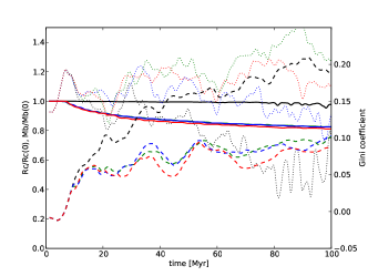
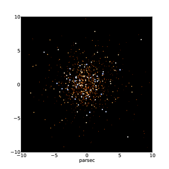
We plot an example of this process (which is similar to figure 6 in Portegies Zwart et al. 2009) in figure 13. For this example we evolve a plummer sphere of $N=1000$ stars with a (homogeneously sampled) Salpeter IMF with lower mass bound of $M=0.3{\rm\thinspace M_{\odot}}$ and upper mass bound of $M=25{\rm\thinspace M_{\odot}}$. The initial core radius is $R_{c}=2$ parsec and the stellar masses are assigned randomly. Runs using different stellar evolution codes, using SSE, EVtwin or MESA, are presented. The first of these is based on look-up tables and interpolation formulae, while the other two are Henyey-type stellar structure solvers. For comparison a run without any stellar evolution is also done. The full stellar evolution codes were run with the SSE fallback option (see section 3.2.1) with a lower limit on the timestep of the stellar evolution code of 1 yr as switching condition. In practice the switch happend around the second asymptotic giant branch stage. As can be seen in Figure 13 the stellar evolution impacts the evolution of the cluster through the mass loss, affecting the evolution of the core radius and the mass segregation. Note that because the coupling is one way, there is no real added value in evaluating the stellar evolution together with the stellar dynamics, other than demonstrating the capabilities of AMUSE. This changes when stars are allowed to merge.

Figure 13: Cluster evolution with live stellar evolution. The upper panel shows the evolution of the core radius (normalized on the initial core radius, dotted lines), bound mass fraction (as fraction of the initial mass, solid lines) and the evolution of the mass segregation as quantified by the Converse & Stahler (2008) “Gini” coefficient (dashed lines) as a function of time for a $N=1000$ star cluster with a salpeter IMF in the case without stellar evolution and in case the stars evolve, calculated with different stellar evolution codes. The black curves are the results for a run without stellar evolution, green are the results for SSE, blue EVtwin and red the MESA stellar evolution code. The middle panel shows the initial distribution of stars (colored according to their temperature and luminosity). The bottom panel shows the Herzsprung-Russell diagram for the stellar evolution as calculated for the different codes (colored as top panel) for the initial population (circles), after 20 Myr (triangles) and after 100 Myr (diamonds).

4.2 Evolution with collisions

Figure 14: Evolution with stellar collisions. Shown is the mass evolution of the most massive merger product for a cluster with top heavy (flat in logarithm) IMF and zero metallicity, and an initial King density profile with $W_{0}=6$ and a virial radius of 0.1 parsec for three runs with the indicated number of stars (see text for details).

Figure 15: Resolving an interaction with the AMUSE multiples module. This diagram shows the resolution of close interactions using the Multiples module. Upper left: if two (possibly compound) objects pass close to each other (as defined by distance $r_{90}<\frac{GM}{\langle v^{2}\rangle}$) control is passed to the Multiples module (right), which transforms to center of mass coordinates and retrieves the internal structure of the particles. It calls a sub code to resolve the collision. Once this is done, the interaction products (which may not correspond to the input systems) are transformed back and returned to the main code (lower left).

Stellar dynamics codes often assume that collisions between stars are rare enough to be unimportant for the evolution of the system. For dense stellar systems this assumption is not correct (Portegies Zwart et al. 1999) and a number of stellar dynamics codes allow for stellar collisions, e.g. Starlab (Portegies Zwart et al. 1999) and Nbody 6 (Nitadori & Aarseth 2012). The AMUSE approach to collision handling is to separate this into two distinct functional tasks: 1) the detection of collisions and 2) the calculation of collision outcomes. Task 1) is most naturally handled in a stellar dynamics code and represents an example of the above mentioned stopping conditions: the interface to dynamics code defines a collision radius $R_{\rm coll}$ - if the code detects a passage of two particles such that they pass closer than $R_{\rm coll}$, the code flags a ‘collision’ stopping condition (such a collision event may be a true collision or a close passage between two bodies in the system) and returns control to the AMUSE framework. The actual calculation of the outcome of a collision is a completely different problem and the appropriate method to resolve this is strongly problem dependent. For a lot of applications a simple ‘sticky particle’ approximation (merging two particles while conserving momentum) may be sufficient, whereas in other cases (e.g. runaway collisions in dense clusters) a more precise characterisation of the internal structure of the collision product is necessary and in this case the collision has to be calculated using more sophisticated codes, e.g. entropy mixing (using MMAS) or a self-consistent SPH stellar collision simulation.

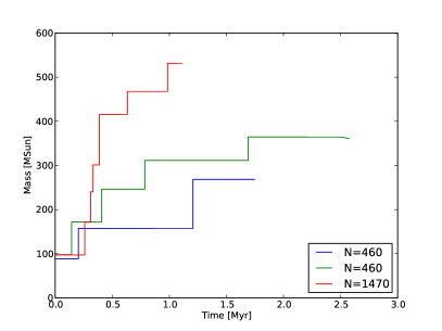
Figure 14 shows an example of the stellar evolution in a star cluster with stellar collisions. For this calculation a model for a dense Pop III star cluster was evolved. Because of the high stellar density and the adapted top-heavy IMF a run-away merger process occurs. The codes that where used in this calculation were: MESA for stellar evolution with zero metallicity stellar models, ph4 for the gravitational dynamics and MMAMS was used to resolve the structure of merger products. Note that in this case the fallback option for stellar evolution is not available - the models were actually stopped as soon as a resulting stellar model did not converge.

4.3 Multiples

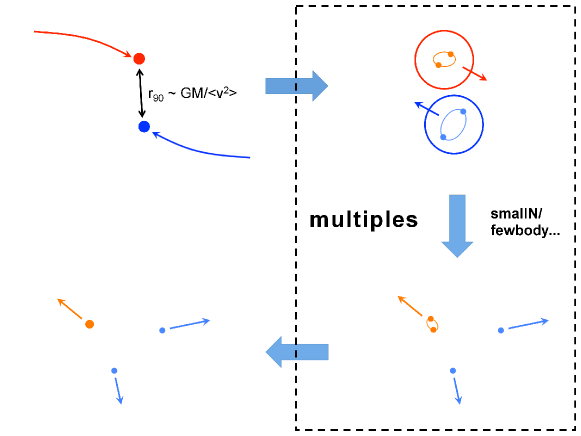
The pattern of collision detection and resolution can also be applied to close passages and low multiples interactions in purely gravitational dynamics in the collisional regime. In this case the collision does not involve physical collisions between stars, but close passages, and the systems involved may be multiple stellar systems. The advantage of resolving these seperately lies in the short timescales of the interactions - handling these by a seperate code can be more efficient, or these interactions may require a different integrator.

Such interactions are handled the same way as the physical collisions above: a parent code detects a close passage (using an interaction radius instead of the physical radius), flags a stopping condition and returns control to the AMUSE framework. Within AMUSE the multiples module implements this type of solver (see fig. 15). The AMUSE framework identifies the particles involved and handles them over to the resolving subcode, which may be for example a Kepler solver, smallN (a code which uses algorithmic regularization) or Mikkola (in case relativistic corrections are important). This code runs until the low N interaction is finished and returns the ‘collision’ products, which may be single stars, stable binaries or hierachical multiples on outgoing trajectories. An additional step may be required to scale back the position to the original interaction radius, since the interactions are assumed to occur instantaneously.

4.4 Bridge integrator

Figure 16: Stable gas plummer sphere test for Bridge. The test consists of evolving a gas Plummer sphere for 10 Nbody times where the hydro forces and self gravity are split over two instances of Fi using Bridge. Left panels show the deviation of the potential (yellow dashed), kinetic (green dotted), thermal (blue dash-dotted) and total energy (red drawn) as a function of time (initial energy values are -0.5, 0, 0.25 and -0.25 respectively). Right panels show the gas density profiles at 10 equally spaced times. Upper panel show results for $N=10^{4}$ particles, while lower panels are for $N=10^{5}$.

The Bridge integrator (Fujii et al. 2007) provides a symplectic mapping for the gravitational evolution in cases were the dynamics of a system can be split in different regimes. The compound nature of the Bridge integrator makes it an ideal target for inclusion within AMUSE and we have implemented a generalized Bridge-type gravitational integrator in AMUSE (see also Portegies Zwart et al. 2013).

The Bridge formulation can be derived from an Hamiltonian splitting argument, as used in planetary dynamics to derive symplectic integrators (Fujii et al. 2007; Wisdom & Holman 1991; Duncan et al. 1998). Consider the Hamiltonian

$$H = \sum_{i\in A\cup B}\frac{p_{i}^{2}}{2m_{i}}+\sum_{i\neq j\in A\cup B}\frac{Gm_{i}m_{j}}{\|{r_{i}-r_{j}}\|}$$ (1)

of a system of particles consisting of subsystems A and B. This can be divided into three parts,

$$H = \sum_{i\in A}\frac{p_{i}^{2}}{2m_{i}}+\sum_{i\neq j\in A}\frac{Gm_{i}m_{j}}{\|{r_{i}-r_{j}}\|}+$$

$$\sum_{i\in B}\frac{p_{i}^{2}}{2m_{i}}+\sum_{i\neq j\in B}\frac{Gm_{i}m_{j}}{\|{r_{i}-r_{j}}\|}+$$

$$\sum_{i\in A,j\in B}\frac{Gm_{i}m_{j}}{\|{r_{i}-r_{j}}\|}$$

$$= H_{A}+H_{B}+H^{int}_{A,B}$$

with $H_{A}$ and $H_{B}$ the Hamiltonians of subsystems A and B respectively and the cross terms are collected in $H^{int}$. The formal time evolution operator of the system can then be written as:

$$e^{\tau H} = e^{\tau/2H^{int}}e^{\tau\left(H_{A}+H_{B}\right)}e^{\tau/2H^{int}}$$ (3)

$$= e^{\tau/2H^{int}}e^{\tau H_{A}}e^{\tau H_{B}}e^{\tau/2H^{int}}.$$

Here the $e^{\tau/2H^{int}}$ operator consists of pure momentum kicks since $H^{int}$ depends only on the positions. The secular evolution part $e^{\tau(H_{A}+H_{B})}$ splits since $H_{A}$ and $H_{B}$ are independent. The evolution of the total system over a timestep $\tau$ can thus be calculated by mutually kicking the component systems A and B. This involves calculating the forces exerted by system A on B and vice versa and advancing the momenta for a time $\tau/2$. Next the two systems are evolved in isolation (each with a suitable method) for a time $\tau$, after which the timestep is finished by another mutual kick.

Within AMUSE, the gravitational dynamics interfaces (table 2) provide for an evolve_model method that can be regarded as an implementation of the secular time evolution operators $e^{\tau H}$. The momentum kicks, on the other hand, are reasonably fast to implement within the framework in Python once the forces are known, and for this the gravitational dynamics interface provides a utility function get_gravity_at_point to query the gravitational forces on arbitrary positions.

Note that the above formulation provides fully symplectic evolution. However in practice the implementation may not be symplectic, because the user is free to choose - and will do so often considering performance - non-symplectic codes for the component integrators and/or approximate methods to calculate the acceleration of the kick operators. Note also that the procedure is not restricted to two systems - the formulation extends to multiple systems by either splitting the Hamiltonian into more parts or applying the above split recursively, and the implementation in AMUSE allows for an arbitrary number of systems.

4.4.1 Gravity-hydrodynamics coupling with Bridge

Figure 17: Energy plot of the Evrard collapse test. Plotted are the kinetic, potential, thermal and total energy as a function of time for runs with Gadget (red dashed: $N=10^{4}$, red drawn: $N=10^{5}$), and for Gadget hydro bridged with Octgrav gravity (blue dash-dotted: $N=10^{4}$, Blue dotted: $N=10^{5}$).

Figure 18: Performance of AMUSE split solvers vs monolithic solvers. Plotted is the ratio of wallclock times using the AMUSE split solver and using the corresponding TreeSPH code (see text for details) as a function of the number $N$ of gas particles.

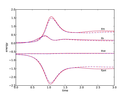
As an illustration of the Bridge integrator and of the tests necessary to verify a coupling strategy within AMUSE, we will present tests of the coupling between gravitational and hydrodynamic SPH systems. The dynamical equations for SPH evolution can also be derived from a Hamiltonian formalism and thus the Bridge formalism directly carries over to a split between purely gravitational and SPH particles  (Saitoh & Makino 2010). We test the Bridge integrator for an equilibrium configuration using a plummer sphere composed of gas, and for the classic Evrard SPH test. In these cases there is no clear spatial or scale separation, and thus this represents a challenging test of the efficiency of the AMUSE framework. A Bridge type integrator for SPH can be implemented in a computationally efficient way within a monolithic code if the time step requirement for the hydrodynamics is more stringent than for the gravitational dynamics (Saitoh & Makino 2010). Below we also test the performance of an implementation within the AMUSE framework.

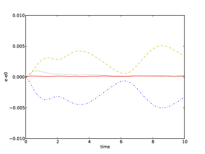
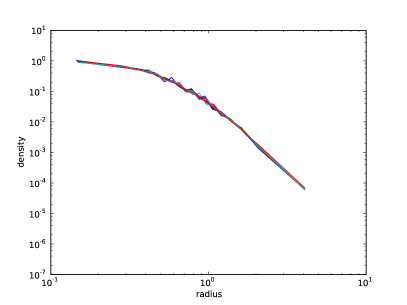
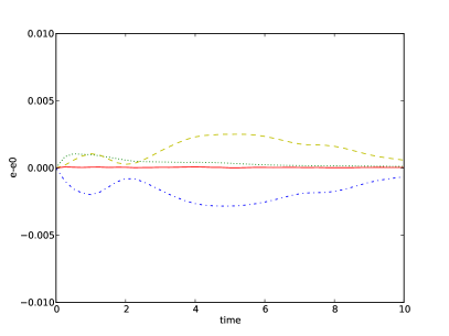
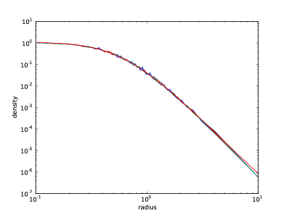
In the test presented in figure 16 we evolve a gas plummer sphere for 10 Nbody times using Bridge with two different instances of Fi: one for the hydrodynamics and one for the self-gravity. The gas initially is at rest and thermally supported and should remain stable. This configuration tests the ability of Bridge to maintain such a stable configuration in spite of the alternation of evolution operators. As can be seen the Bridge integrator conserves energy and maintains the equilibrium gas distribution satisfactorily to within $\sim 0.1\%$. A slight relaxation of the initial conditions is visible.

The second Bridge test consists of a dynamic test where we conduct the classic (Evrard 1988) test of a collapsing gas sphere. We compare the results of the test using a conventional TreeSPH code (Gadget) with a Bridge solver where different codes are used to calculate the hydrodynamics and the self-gravity (in this case the self-gravity of the SPH code is turned off). As can be seen in figure 17 essentially the same results are obtained using the Bridge solver and the monolithic solver.

We also examine the performance of the hydrodynamics-gravity coupling using the Bridge integrator. Saitoh & Makino (2010) showed that for an implementation of Bridge within a single code, performance gains were possible due to the fact that the gravitational and hydrodynamic force evaluations were better matched with their respective timestep criteria. Although performance is not the prime motive for AMUSE, this kind of coupling represents a challenge due to the strong coupling between the different sub systems, so it is instructive to see how the performance of AMUSE compares with using a monolithic code.

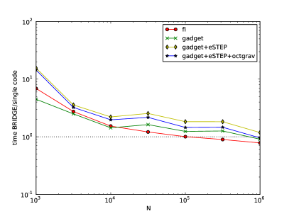
The simulations performed start out with a plummer sphere of mixed gas and star particles, with $1000$ equal mass star particles and a varying number of gas particles. The run time is compared with a monolithic code (either Fi or Gadget) performing the same calculation. Because these codes are targeted to collisionless dynamics, the stellar gravitational interactions were smoothed using a smoothing length $\epsilon=0.01$ (in Nbody units).

Figure 19: Solver for planetary interactions. Plotted are different frames of a test simulation where circles are drawn around each center of mass node in the parent integrator (Hermite0), where the linestyle indicates the type of subnode: black solid indicates a single particle in the parent code, blue dotted a two-body Kepler solver, green dash-dotted a general N-body code (Huayno) and red dashed a symplectic planetary integrator (Mercury). The green dots are stellar systems, the plusses are planets.

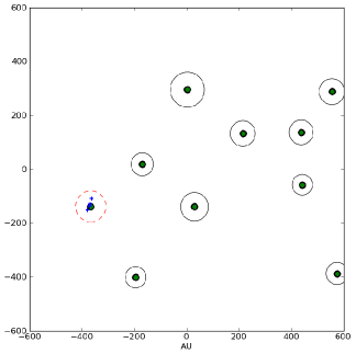
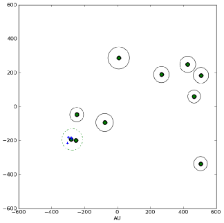
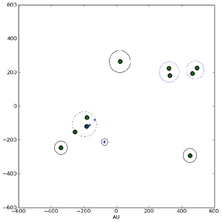
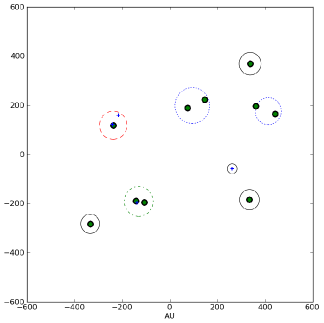
Figure 18 shows the timing results for 4 different simulation sets, which are labelled with the code used: Fi on a 4 core workstation, Gadget using 4 MPI processes on one workstation, Gadget split over 2 workstations using eSTeP and Gadget split over 2 workstations using eSTeP while using the GPU code Octgrav on a different machine to calculate gravity. As can be seen in the figure the overhead of using AMUSE is large for small N. This is to be expected: each call in the framework is transported using either MPI or eSTeP, which is considerably more costly than an in-code function call. However, increasing the number of particles the relative overhead of the AMUSE framework goes down and for $N=10^{6}$ the AMUSE split solvers are competetive with the monolithic code. The reason for this is that the communication scales at most linearly with $N$, while the scaling of the computation goes as $N\ {\rm log}\ N$. Noting the two runs with eSTeP, we see that this imposes an extra overhead. However if running on multiple machines entails a more efficient use of resources (here exemplified by using a GPU enabled treecode to calculate the gravity) spreading out the computation on machines with different architectures can also increase the efficiency of the computation (although for this particular problem not enough to offset the communication cost).

4.5 Strong and weak coupling of planetary systems in clusters

The Bridge integrator is suitable for problems where one or a small number of composite particles is embedded in a larger system. A limitation of the normal bridge is the fact that the interactions between a composite particle and the rest of the system are calculated using 2nd order leap-frog splitting. When most or all ‘particles’ in a larger system are compound, say a cluster of stars where the stars are multiple systems or have planets orbiting them, the Bridge integrator is equivalent to a 2nd order leap-frog implemented in Python. Furthermore, in this case it is possible that compound systems will encounter each other and interact, so provisions for this have also to be made.

For such a case one can formulate a variant of bridge where all particles, including the compound particles, are evolved in a parent code (which can be e.g. a high order Hermite code). The compound particles have a representation in the parent code in the form of a center of mass particle with an associated interaction radius. This center of mass particle is evolved in the parent code, while the compound subsystem is evolved by a different code, with perturbations due to the rest of the system. The perturbations consist of periodic velocity kicks. Subsystems are allowed to merge if they pass close to each other (using the collision stopping condition of the parent code) and can be split if seperate associations within the subsystem are identified. Such a method is implemented in the Nemesis integrator (Geller et al., in prep.). Figure 19 shows an example, where we evolve a random configuration of stars (the initial condition is chosen planar for clarity, so it does not represent any realistic object), with initially one compound system (the sun with the outer gas giants). As the stars evolve, the integrator detects close passages between systems, identifies subsystems and decides dynamically the most suitable integrator for such a system, choosing a Kepler solver if the subsystem consists of two bodies, the solar system integrator Mercury when the heaviest particle is more than a factor 100 heavier than the second most massive particle or the Huayno integrator otherwise.

Although the Nemesis integrator and the Multiples module (section 4.3) have similar goals, they differ in the handling of compound systems. Interactions in the Nemesis code proceed on the same timeline as the parent system (it is not assumed to be resolved instantaneously) and feel (albeit in a perturbation sense) the large scale density distribution, while for Multiples the interactions are resolved in isolation and instantaneously. This does result in more stringent timestepping constraints for the Nemesis integrator, though.

4.6 Gravitational dynamics and hydrodynamics with stellar feedback

Figure 20: AMUSE gravitational/hydrodynamic/stellar evolution integrator. This diagram shows the calling sequence of the different AMUSE elements in the combined gravitational/hydro/stellar solver during a time step of the combined solver. Circles indicate calls to the (optimized) component solvers, while rectangles indicate parts of the solver implemented in Python within AMUSE (from Pelupessy & Portegies Zwart 2012).

The cluster simulations with stellar evolution of section 4.1 assumed the clusters consisted of stars only. This is not a good approximation for the earliest phase after the formation of a cluster, when the cluster is still embedded in the gas cloud from which it formed. In this case the interplay of stellar evolution, hydrodynamics and stellar dynamics becomes more complicated because young massive stars inject energy into the surrounding gas medium by stellar winds and supernovae. This has a drastic effect on the gas dynamics, which in turn affects the stellar dynamics.

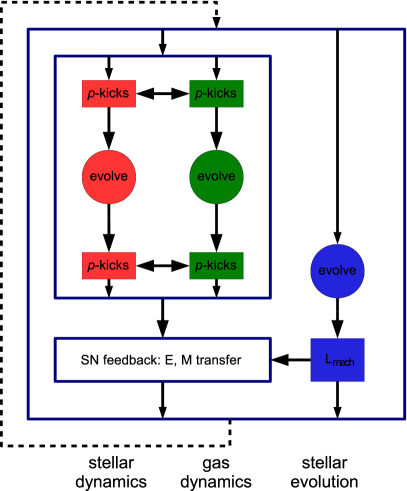
The coupling between hydrodynamics and gravity is a special case of Bridge (see section 4.4). The feedback from stellar winds and supernovae can be implemented as energy source terms for the gas dynamics, where the mechanical luminosity $L_{\rm mech}$ is determined by the stellar evolution and parametrized mass loss rates and terminal wind velocities (e.g. Leitherer et al. 1992; Prinja et al. 1990). The calling sequence of a combined gravitational/hydrodynamic/stellar evolution integrator is shown in figure 20. This integrator was used to study the early survival of embedded clusters (see section 5.2)

4.7 Radiative hydrodynamics

Another example of a close coupling is the interaction of radiation and hydrodynamics. In the general case, this is an example of a type of problem where a dedicated coupled solver may be necessary, but in many astrophysical applications an operator-splitting approximation is reasonably efficient. The operator splitting for system governed by radiative hydrodynamic equations can be effected in a ‘leap-frog’ fashion: to advance a given system from time $t$ to $t+\Delta t$, a hydrodynamic solver is first advanced for a half step $\Delta t/2$ and then communicates its state variables at $t+\Delta t/2$ to the radiative transfer code. The radiative transfer code proceeds evolving the radiation field, internal energy, ionization, etc, taking a full integration step. The internal energy from the radiative transfer code (at $t+\Delta t$) is then used to update internal energy of the hydrodynamics code, which then advances to $t+\Delta t$, completing the timestep. This approximation holds as long as the effects from the finite speed of light can be ignored, and as long as $\Delta t$ is small enough that the reaction of the gas flow to the radiation field can be followed. We illustrate this simple scheme with an integrator based on an analytic cooling prescription (sec. 4.7.1) and an integrator using a full radiative transfer code (sec. 4.7.2).

4.7.1 Thermally unstable ISM

Figure 21: Simulations of a thermally unstable ISM model. Upper panels show slices of the density field for the Athena grid code (left) and the SPH code Fi (right) after 0.5 Myr of evolution. In both cases the thermal evolution is calculated using constant heating and the simple analytic Gerritsen & Icke (1997) cooling curve, resulting in a thermally unstable model. This can be seen in the (equilibrium) density-pressure relation (lower left panel). In the lower right panel we show the evolution of the cool ( $T<100$ K, blue lines) and dense ($\rho>10$ cm^-3, red lines) gas fractions, where the solid lines show the results for Athena, dash-dotted those of Fi. Both models show broadly similar behaviour, although clearly differences can be seen, which must be traced to the use of different numerical hydrodynamic solvers.

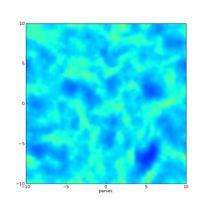
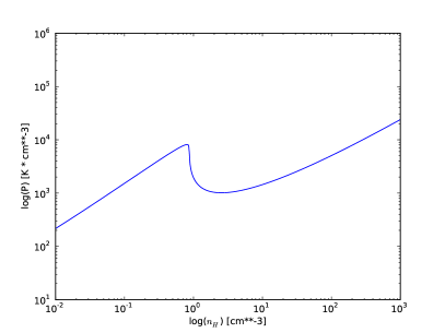
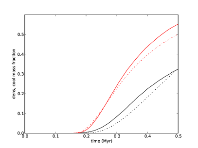
Probably the simplest case of this coupling concerns the cooling of the ISM in optically thin atomic cooling lines in the low density limit. In this case the radiative coupling can be described with a cooling function $\Lambda$, which is a function of the temperature $T$ for which various tabulations exist. Here we will use a simple analytic approximation (Gerritsen & Icke 1997),

$$\Lambda(T) = 10^{-21}\times\left(10^{(-0.1-1.88*(5.23-log(T))**4)}+\right.$$

$$\ \ \ \left.10^{(-3.24-0.17*|(4-log(T)|)**3)}\right){\rm\ erg\ cm}^{3}/{\rm s}$$

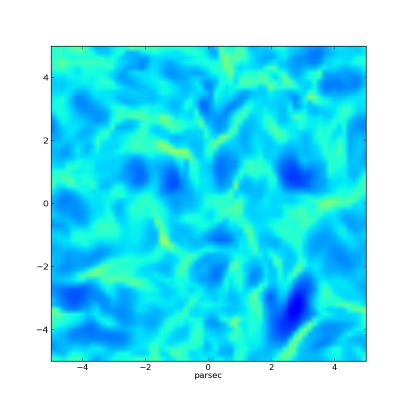
with a constant heating $\Gamma=0.05\times 10^{-23}n\ {\rm ergs}/{\rm cm}^{3}/{\rm s}$. While highly idealized, this results in a classic Field (1965) two phase instability, as can be seen in the equilibrium density pressure relation in figure 21. The dynamical effect of this instability in a turbulent ISM can be explored with the operator splitting radiative hydro scheme. An example of this is shown in figure 21, where we have set up a periodic box 10 parsec accross with initially a uniform density $n=1.14\ {\rm cm}^{-3}$, temperature $T=8000\ K$ and a divergence free turbulent velocity spectrum with velocity dispersion $\sigma=8\ {\rm km}/{\rm s}$. We compare two completely different hydrodynamic methods, namely the SPH code Fi and the finite volume grid solver Athena. Because the initial conditions of the former consist of particles, while the latter is a grid code, some care must be taken in generating equivalent initial conditions. Here the initial hydrodynamic state grid for Athena was generated by sampling the hydrodynamic state from the SPH code. The thermal evolution was solved in Python by a simple ODE solver for the thermal balance. As can be seen in the snapshots shown in figure  21 the two methods give qualitatively similar results, but clearly the chosen numerical method affects the details.

4.7.2 Dynamic Iliev tests

Figure 22: Test 5 of Iliev et al. (2009): ionization front expansion in an initially homogeneous medium. Shown are plots of the ionization fraction $x$ (top left panel), temperature T (top right) and the density profile (bottom) as a function of the distance (normalized on the box size $L_{\rm box}$) to a source with a luminosity $L=5\times 10^{48}{\rm s}^{-1}$ after 10, 30 and 200 Myr of evolution (for density only the 200 Myr case is shown). Blue line: Fi with SimpleX, green: Gadget2 with SimpleX, yellow: Fi with SPHRay, red: Gadget2 with SPHRay.

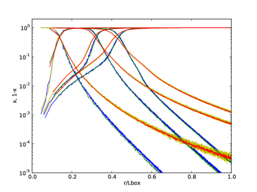
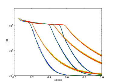
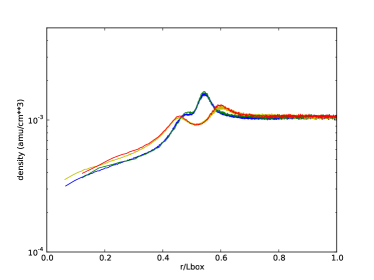
The leap-frog coupling scheme described above for optically thin cooling and heating can be applied also for the more computationally expensive case of the transport of ionizing radiation in an optically thick medium. In this case, instead of a simple ODE solver using only local information, the full radiation transport must be solved for the internal energy integration. Thus a radiative hydrodynamics solver can be constructed within AMUSE by coupling seperate hydrodynamic and radiative transfer solvers.

In figure 22 we show the result of an application of this coupling. Here we perform a test described in a comparison paper of different radiative-hydrodynamics codes (Iliev et al. 2009). This test (test 5 of Iliev et al. 2009) involves the calculation of the HII front expansion in an initially homogeneous medium. We evaluated the four different possible combinations of the two SPH codes (Fi and Gadget2) and the two radiative transfer codes (SPHRay and SimpleX) currently interfaced in AMUSE. Figure 22 shows the resulting evolution of the ionization structure, temperature and density for the 4 different solvers. The resulting HII front expansion falls within the range of solutions encountered in Iliev et al. (2009). Both radiative codes show different behaviour in the fall-off of the ionization and temperature. This is due to differences in the treatment of the high energy photons in SPHRay and SimpleX. A similar scatter in the profiles ahead of the ionization front is encountered in Iliev et al. (2009). Note that the hydrodynamic code chosen has relatively little impact on the resulting profiles, since both codes are SPH codes. A more quantitive examination of the radiative hydrodynamics coupling within AMUSE is in preparation (Clementel et al.).

5 Applications

A number of studies have been conducted using AMUSE, amongst which an examination of the origin of the millisecond pulsar J1903$+$0327, a pulsar with a companion in an unusually wide and eccentric orbit (Portegies Zwart et al. 2011). Here, AMUSE was used to resolve triple interactions. Whitehead et al. (2011) examined the influence of the choice of stellar evolution model on cluster evolution using AMUSE. The Huayno integrator (Pelupessy et al. 2012) was developed within AMUSE. Kazandjian et al. (2012) studied the role of mechanical heating in PDR regions. Here AMUSE was used as a driver to conduct parameter studies. In Portegies Zwart (2013) AMUSE was used in order to resolve stellar evolution and planetary dynamics after the common envelope phase in binary systems with planets. Whitehead et al (2013, in prep.) used AMUSE to examine stellar mass loss and its effect on cluster lifetimes. We will examine three other applications in some detail below, as they provide instructive case studies.

5.1 Globular clusters in realistic galaxy potentials

Figure 23: Simulations of a globular cluster: comparison of Tree and direct Nbody codes. Evolution of the bound mass (top panel) and the 90%, 50% and 1% Lagrangian radii (top to bottom, bottom panel) of a simulated star cluster subject to a galactic tidal field extracted from a cosmological simulation (model A12-2 from Rieder et al. (2012, submitted)). The cluster was simulated with the GPU treecode Bonsai (red, solid curves) and Hermite direct N-body code ph4 (blue, dashed curve). From Rieder et al. (2012).

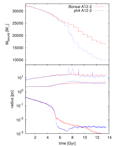
Rieder et al. (2012, submitted) studied the evolution of globular clusters in cosmological density fields. For this study realistic tidal fields extracted from the CosmoGrid simulation (Ishiyama et al. 2013) were used as the time varying background potential against which globular cluster models were evolved using the Bridge integrator. Technically this means that a minimal gravity interface - only consisting of get_gravity_at_point and get_potential_at_point and an evolve_model method which interpolates against precomputed tidal field tensors - is constructed for use in the Bridge integrator.

Fig. 23 presents the mass and the Lagrangian radii of a simulated cluster as a function of time, for the two codes Bonsai and ph4. For most of the simulations in the paper Bonsai, a treecode running on the GPU, was used, because the main interest of the authors was in the survivability of the cluster, and not in the details of the internal structure of the clusters. However, in order to validate the use of the tree code, the simulations were tested against runs with the direct Hermite N-body code ph4, only changing the core integrator. As can be seen in Figure 23 the difference in mass evolution between ph4 and Bonsai remains quite small until about 5Gyr. After this moment, both clusters go into core collapse. Until about 8.5Gyr, the ph4 cluster displays much higher mass loss than the Bonsai cluster as it expands following core collapse. After 8.5Gyr, both codes again show similar behaviour. The Lagrangian radii of the clusters are nearly equal until core collapse occurs at about 5Gyr. After this, the core collapse is initially deeper in ph4, while after 8.5Gyr Bonsai reaches the same depth. From these results, the authors inferred that the Bonsai simulations were not as well suited for determining the internal structure evolution of the star clusters as ph4 would be. However, the effect of the external cosmological tidal field remains largely unchanged between ph4 and Bonsai. Since the main interest in the study was the mass evolution of the clusters due to the tidal field, Bonsai was considered adequate to give an indication of the effect of tidal fields on the cluster mass loss.

5.2 Embedded cluster evolution

Figure 24: Evolution of the stellar and gas distribution of an embedded cluster, including stellar evolution and feedback from stellar winds and supernovae. Snapshots are labelled with their time in the lower right corner. Shown as a density plot is a slice through the midplane of the gas density. Stars are divided in 4 mass bins: $m_{\star}\leq 0.9{\rm\thinspace M_{\odot}}$ (smallest red dots), $0.9{\rm\thinspace M_{\odot}}\leq m_{\star}\leq 2.5{\rm\thinspace M_{\odot}}$ (intermediate yellow dots), $2.5{\rm\thinspace M_{\odot}}\leq m_{\star}\leq 10{\rm\thinspace M_{\odot}}$ (intermediate green dots) and $m_{\star}\geq 10{\rm\thinspace M_{\odot}}$ (large light blue dots). From Pelupessy & Portegies Zwart (2012).

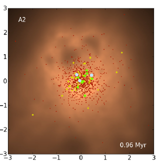
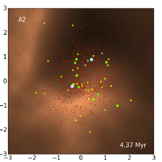
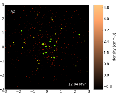
Stellar clusters form embedded in the natal cloud of gas with star formation efficiencies (the fraction of mass that end up in stars) of about 5%-30% (Williams & McKee 1997). The energy output from all the massive stars typically exceeds the total binding energy of the embedded star cluster. The loss of gas from the embedded proto-cluster may cause the young cluster to dissolve (Hills 1980; Lada et al. 1984). The survivability of the cluster depends on the efficiency with which the radiative, thermal and mechanical energy of the stellar outflows couple to the inter-cluster gas, and these are determined by stellar evolution processes. Therefore in order to fully represent the evolution from its embedded to a gas free and more evolved state one needs to take into account various physical ingredients. This problem was examined by Pelupessy & Portegies Zwart (2012). AMUSE was used because of the need of combining gas dynamics with high precision N-body dynamics and stellar evolution. The combined solver described in section 4.6 was developed for this purpose. The resulting script consists of a number of components that can be reused in other settings (see fig. 20), and are also flexible in the choice of core integrators. In this case the hydrodynamics of the gas was calculated using an SPH code (Gadget), gravitational dynamics was calculated using a 4th order Hermite N-body solver (PhiGRAPE) while the cross coupling was done using a tree- gravity solver (Octgrav). The mechanical luminosity of the stars was calculated using the results of the stellar evolution code SSE, using the stellar radii and temperatures and empyrical relations for the terminal wind velocities (Leitherer et al. 1992; Prinja et al. 1990), this - together with the supernova energy and mass loss determined the energy and mass injection into the cluster medium. Figure 24 shows snapshots of an example simulation (model A2 of Pelupessy & Portegies Zwart (2012)).

5.3 Circumbinary disks

Figure 25: Circumbinary disk simulation for a model matching the parameters of Kepler 34, from Pelupessy & Portegies Zwart (2013). Shown is the distribution of gas in the semi-major axis - eccentricity plane with the orbital parameters of the observed planet around Kepler 34 as the blue dot (with the range of semi-major axis and eccentricity encountered during long term integrations given by the error bars). The stability of planetary orbits is indicated by the red crosses and plusses, where these indicate the unstable models from a grid of models calculated with AMUSE.

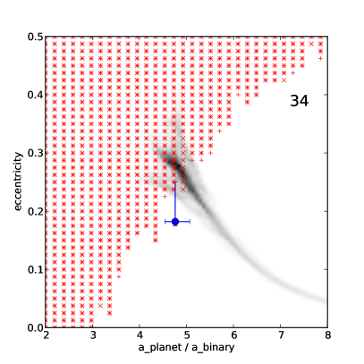
Pelupessy & Portegies Zwart (2013) examined the formation of planets around binary stars. This study used AMUSE to answer two different questions, namely: what is the hydrodynamic reaction of a disk centered on the components of a binary and secondly what is the (approximate) region of stability (in semi-major axis - eccentricity space) for planets around circumbinary systems. For the hydrodynamic simulations the binary parameters were chosen to match a set of recently detected binary systems with planetary systems orbiting both components (Doyle et al. 2011; Welsh 2012) and for a set chosen from a survey of eclipsing binaries (Devor et al. 2008). The gas turned out to settle in a disk with increasing eccentricity towards the center of the disk (fig. 25). To explore the question whether planets formed from the gas disk would be in stable orbits, a grid of three-body models was run for each system, where for varying planetary semi-major axis, eccentricity and pericentric angle a three-body initial condition was integrated for 1 Myr using a high precision N-body code (Huayno). These runs are also summarized for Kepler 34 in figure 25. Each of these models take a non-trivial amount of time (in the order of 30 min). In order to speed up the calculation these jobs where farmed out over different work-stations using the AMUSE remote running functionality (see section 2.1.2).

6 Discussion

The AMUSE framework provides an environment for conducting multi-physics computational experiments in Astrophysics. We have presented the design, the core modules and an overview of the different coupling strategies that can be employed within AMUSE. We have presented applications of the AMUSE framework that show different aspects of the usage of the framework. AMUSE is an easy platform for computational experiments, where the barrier of using different codes is lowered by standardizing IO and the calling sequence. Coupling different codes and physical processes or regimes is made transparent by automatic unit conversion and restricting the interface communication to physically relevant quantities. Finally, the remote callability of the interfaces allows for scalable computing.

An additional important aspect of AMUSE is that it encourages reproducibility in computational experiments: the source of the framework and the community codes are distributed in an open source package. The scripts describing the computational experiments can be easily communicated and by allowing to easily change between different solvers and numerical methods it enables routine cross verification of calculations.

The current design of AMUSE has a number of limitations which must be kept in mind when using the framework and designing numerical experiments. Currently AMUSE uses a centralized message system, where all the communication passes through and is initiated by the master user script. This means that ultimately the scripts will be limited by the communication bandwidth of the machine where the user script is started. Even if the communication only concerns, for example, a gravity and a hydro-code started on different machines exchanging information, this communication has to pass through the master script’s machine, and will block the script from performing other taks. This can be mitigated in the current design by encapsulating such tasks and sending them off as one unit and by using threading in the master script. A different solution we will explore in the future is to implement communication channels using tangential communication paths. The fact that the communication is always initiated by the master script imposes a limitation on the algorithms implemented in AMUSE. It is for example difficult to implement a coupling using adaptive individual time-stepping. In the future, a call-back mechanism, whereby a community code can put in requests for communication, could solve this.

In spite of these limitations there is a large class of problems to which AMUSE can be applied productively. It is instructive to compare the AMUSE approach to coupling codes with two conventional ways in which codes are coupled: namely using simple command line scripting, using e.g. UNIX pipes, and native implementations where codes are coupled on the source code level. Command line scripting is used often in astrophysical simulations, and mostly for input/output coupling. Looking back at the other couplings in section 4, it is clear that these are progressively more cumbersome to implement using pure command line scripting, needing more and more ad-hoc constructs. On the other hand, writing a native solver is the preferred method for tightly coupled physics. However as one progresses towards more loosely coupled domains this becomes more cumbersome from the viewpoint of modularity and flexibility.

6.1 Testing and verification

The source code includes more than 2065 automatic tests. These unit tests test aspects of the core framework as well as the community interfaces. Coverage of the tests (the fraction of the code that is executed during the tests) is 80%. The source code is maintained in an SVN repository and the test suite is executed for every change in the source code base, and daily on a selection of (virtual) test machines. The tests cover the base framework code, support libraries and community code interfaces, where for the latter the base functionality of the interfaces is checked.

In addition, to assess the utility of AMUSE for realistic scientific problems, the code is also validated against published results. Most of the framework code in AMUSE can be tested with the unit tests, but these only test if a small part of the code works as planned. The unit test do not tell the user anything about the accuracy or the validity of an AMUSE solver. Validation against existing problems provides more insight. For these validation tests we select test problems which only use physics implemented in AMUSE, provide a challenging test of one or more modules, and are well defined and possible to implement using easily generated data and initial conditions, but not too expensive computationally. Examples of such test problems are: Bonnell et al. (2003): cluster formation, Fujii et al. (2007): galaxy/ cluster interaction, Glebbeek et al. (2009): evolution of runaway stellar collision products, Iliev et al. (2009): radiative comparison tests, Mellema et al. (2002): cloud$/$shock interactions.

Finally, we want to caution that the above tests do not mean that the framework will give correct and meaningful results under all circumstances. Developing a new application for AMUSE entails careful testing, especially when new physical regimes are probed.

6.2 Performance

A general statement about the performance of AMUSE is difficult to make, since such a wide variety of types of numerical experiments can be conducted. The design of AMUSE does take into account efficiency, using array operations as much as possible for communication, basing storage in Python on Numpy arrays and minimizing the use of relatively expensive data structures (such as Python dictionaries). The community solvers on the other hand are usually well optimised, and a large class of problems spend only a tiny fraction of their time in the framework. In these cases the performance of the framework is certainly not a concern. Experiments in section 4.4 (and also in Portegies Zwart et al. 2013) show that even in relatively tightly coupled problems, where intensive communication is needed between the component solvers, good performance (compared to monolithic solvers) is possible. As we mentioned above however, the current design does impose limitations for very large problems.

6.3 Extending AMUSE

The main framework and community modules are production ready, however AMUSE is foreseen to grow over time with new codes and capabilities. AMUSE is freely downloadable and can easily be adapted for private use or extensions may be submitted to the repository, a practice we want to encourage by providing a mechanism whereby at the end of an AMUSE script the framework provides the references for the community codes used.

In our experience writing an interface to a new code, which also involves writing tests and testing and debugging the interface, represents a modest amount work. While every code is different and has its own peculiarities, it is typically something that can be finished during a short working visit or small workshop. Defining an interface for a new domain can take longer, as these need refinement over time.

7 Conclusions

We present the Astrophysical Multipurpose Software Environment (AMUSE). AMUSE as an environment presents a wide variety of astrophysical codes using homogeneous interfaces, simplifying their use. It allows the design of computational experiments with multiple domains of physics spanning a wide range of physical scales using heterogeneous computing resources. It allows for rapid development, encouraging the creation of simple scripts, but its core design is suitable for deployment in high performance computing environments. It enables cross verification of simulations by allowing experiments to be repeated trivially easy with different codes of similar design, or using wholly different numerical methods. It fosters reproducibility in numerical experiments by reducing complicated coding to self-contained and easily portable scripts.

acknowledgements This work was supported by the Netherlands Research Council NWO (grants #643.200.503, #639.073.803 and #614.061.608) and by the Netherlands Research School for Astronomy (NOVA). We would like to thank the following people for contributing figures: Jürgen Jänes (figure 8), Steven Rieder (figure 23) and Nicola Clementel (figure 22).

References

- Agertz et al. (2007) Agertz, O., Moore, B., Stadel, J., et al. 2007, MNRAS, 380, 963
- Altay et al. (2008) Altay, G., Croft, R. A. C., & Pelupessy, I. 2008, MNRAS, 386, 1931
- Barnes & Hut (1986) Barnes, J. & Hut, P. 1986, Nature, 324, 446
- Bate et al. (1971) Bate, R. R., Mueller, D. D., & White, J. E. 1971, Fundamentals of astrodynamics.
- Bédorf et al. (2012) Bédorf, J., Gaburov, E., & Portegies Zwart, S. 2012, Journal of Computational Physics, 231, 2825
- Bonnell et al. (2003) Bonnell, I. A., Bate, M. R., & Vine, S. G. 2003, MNRAS, 343, 413
- Capuzzo-Dolcetta et al. (2013) Capuzzo-Dolcetta, R., Spera, M., & Punzo, D. 2013, Journal of Computational Physics, 236, 580
- Chambers (1999) Chambers, J. E. 1999, MNRAS, 304, 793
- Converse & Stahler (2008) Converse, J. M. & Stahler, S. W. 2008, ApJ, 678, 431
- Devor et al. (2008) Devor, J., Charbonneau, D., O’Donovan, F. T., Mandushev, G., & Torres, G. 2008, AJ, 135, 850
- Doyle et al. (2011) Doyle, L. R., Carter, J. A., & Fabrycky, D. C. e. a. 2011, Science, 333, 1602
- Drost et al. (2012) Drost, N., Maassen, J., van Meersbergen, M. A. J., et al. 2012, in IPDPS Workshops (IEEE Computer Society), 150–162
- Duncan et al. (1998) Duncan, M. J., Levison, H. F., & Lee, M. H. 1998, AJ, 116, 2067
- Eggleton (1971) Eggleton, P. P. 1971, MNRAS, 151, 351
- Eisenstein & Hut (1998) Eisenstein, D. J. & Hut, P. 1998, ApJ, 498, 137
- Ercolano et al. (2003) Ercolano, B., Barlow, M. J., Storey, P. J., & Liu, X.-W. 2003, MNRAS, 340, 1136
- Evrard (1988) Evrard, A. E. 1988, MNRAS, 235, 911
- Field (1965) Field, G. B. 1965, ApJ, 142, 531
- Fryxell et al. (2000) Fryxell, B., Olson, K., Ricker, P., et al. 2000, ApJS, 131, 273
- Fujii et al. (2007) Fujii, M., Iwasawa, M., Funato, Y., & Makino, J. 2007, PASJ, 59, 1095
- Gaburov et al. (2010) Gaburov, E., Bédorf, J., & Portegies Zwart, S. 2010, Procedia Computer Science, volume 1, p. 1119-1127, 1, 1119
- Gaburov et al. (2008) Gaburov, E., Lombardi, J. C., & Portegies Zwart, S. 2008, MNRAS, 383, L5
- Gerritsen & Icke (1997) Gerritsen, J. P. E. & Icke, V. 1997, A&A, 325, 972
- Giersz (2006) Giersz, M. 2006, MNRAS, 371, 484
- Glebbeek et al. (2009) Glebbeek, E., Gaburov, E., de Mink, S. E., Pols, O. R., & Portegies Zwart, S. F. 2009, A&A, 497, 255
- Glebbeek et al. (2008) Glebbeek, E., Pols, O. R., & Hurley, J. R. 2008, A&A, 488, 1007
- Goodwin & Whitworth (2004) Goodwin, S. P. & Whitworth, A. P. 2004, A&A, 413, 929
- Groen et al. (2012) Groen, D., Zasada, S. J., & Coveney, P. V. 2012, ArXiv e-prints
- Harfst et al. (2007) Harfst, S., Gualandris, A., Merritt, D., et al. 2007, New Astronomy, 12, 357
- Henyey et al. (1964) Henyey, L. G., Forbes, J. E., & Gould, N. L. 1964, ApJ, 139, 306
- Henyey et al. (1959) Henyey, L. G., Wilets, L., Böhm, K. H., Lelevier, R., & Levee, R. D. 1959, ApJ, 129, 628
- Hernquist & Katz (1989) Hernquist, L. & Katz, N. 1989, ApJS, 70, 419
- Hills (1980) Hills, J. G. 1980, ApJ, 235, 986
- Hurley et al. (2000) Hurley, J. R., Pols, O. R., & Tout, C. A. 2000, MNRAS, 315, 543
- Hut et al. (1995) Hut, P., Makino, J., & McMillan, S. 1995, ApJ, 443, L93
- Iliev et al. (2009) Iliev, I. T., Whalen, D., Mellema, G., et al. 2009, MNRAS, 400, 1283
- Ishiyama et al. (2013) Ishiyama, T., Rieder, S., Makino, J., et al. 2013, ApJ, 767, 146
- Iwasawa et al. (2011) Iwasawa, M., An, S., Matsubayashi, T., Funato, Y., & Makino, J. 2011, ApJ, 731, L9
- Kazandjian et al. (2012) Kazandjian, M. V., Meijerink, R., Pelupessy, I., Israel, F. P., & Spaans, M. 2012, A&A, 542, A65
- Keppens et al. (2012) Keppens, R., Meliani, Z., van Marle, A., et al. 2012, Journal of Computational Physics, 231, 718 , special Issue: Computational Plasma Physics
- Lada et al. (1984) Lada, C. J., Margulis, M., & Dearborn, D. 1984, ApJ, 285, 141
- Leitherer et al. (1992) Leitherer, C., Robert, C., & Drissen, L. 1992, ApJ, 401, 596
- Mellema et al. (1991) Mellema, G., Eulderink, F., & Icke, V. 1991, A&A, 252, 718
- Mellema et al. (2002) Mellema, G., Kurk, J. D., & Röttgering, H. J. A. 2002, A&A, 395, L13
- Mikkola & Merritt (2008) Mikkola, S. & Merritt, D. 2008, AJ, 135, 2398
- Nitadori & Aarseth (2012) Nitadori, K. & Aarseth, S. J. 2012, MNRAS, 424, 545
- Paardekooper et al. (2010) Paardekooper, J.-P., Kruip, C. J. H., & Icke, V. 2010, A&A, 515, A79
- Paxton et al. (2011) Paxton, B., Bildsten, L., Dotter, A., et al. 2011, ApJS, 192, 3
- Pelupessy (2005) Pelupessy, F. I. 2005, PhD thesis, Leiden Observatory, Leiden University, P.O. Box 9513, 2300 RA Leiden, The Netherlands
- Pelupessy et al. (2012) Pelupessy, F. I., Jänes, J., & Portegies Zwart, S. 2012, New A, 17, 711
- Pelupessy & Portegies Zwart (2012) Pelupessy, F. I. & Portegies Zwart, S. 2012, MNRAS, 420, 1503
- Pelupessy & Portegies Zwart (2013) Pelupessy, F. I. & Portegies Zwart, S. 2013, MNRAS, 429, 895
- Portegies Zwart (2013) Portegies Zwart, S. 2013, MNRAS, 429, L45
- Portegies Zwart et al. (2009) Portegies Zwart, S., McMillan, S., Harfst, S., et al. 2009, New Astronomy, 14, 369
- Portegies Zwart et al. (2013) Portegies Zwart, S., McMillan, S. L. W., van Elteren, E., Pelupessy, I., & de Vries, N. 2013, Computer Physics Communications, 183, 456
- Portegies Zwart et al. (2011) Portegies Zwart, S., van den Heuvel, E. P. J., van Leeuwen, J., & Nelemans, G. 2011, ApJ, 734, 55
- Portegies Zwart et al. (1999) Portegies Zwart, S. F., Makino, J., McMillan, S. L. W., & Hut, P. 1999, A&A, 348, 117
- Portegies Zwart et al. (2001) Portegies Zwart, S. F., McMillan, S. L. W., Hut, P., & Makino, J. 2001, MNRAS, 321, 199
- Prinja et al. (1990) Prinja, R. K., Barlow, M. J., & Howarth, I. D. 1990, ApJ, 361, 607
- Saitoh & Makino (2010) Saitoh, T. R. & Makino, J. 2010, PASJ, 62, 301
- Seinstra et al. (2011) Seinstra, F. J., Maassen, J., van Nieuwpoort, R. V., et al. 2011, Jungle Computing: Distributed Supercomputing Beyond Clusters, Grids, and Clouds, ed. M. Cafaro & G. Aloisio, 167
- Springel (2005) Springel, V. 2005, MNRAS, 364, 1105
- Springel et al. (2001) Springel, V., Yoshida, N., & White, S. D. M. 2001, New Astronomy, 6, 79
- Stone et al. (2008) Stone, J. M., Gardiner, T. A., Teuben, P., Hawley, J. F., & Simon, J. B. 2008, ApJS, 178, 137
- Teuben (1995) Teuben, P. 1995, in Astronomical Society of the Pacific Conference Series, Vol. 77, Astronomical Data Analysis Software and Systems IV, ed. R. A. Shaw, H. E. Payne, & J. J. E. Hayes, 398–+
- Welsh (2012) Welsh, W.F., e. a. 2012, Nature
- Whitehead et al. (2011) Whitehead, A. J., McMillan, S. L. W., Portegies Zwart, S., & Vesperini, E. 2011, in American Astronomical Society Meeting Abstracts #218, #133.10
- Whitworth (1998) Whitworth, A. P. 1998, MNRAS, 296, 442
- Widrow et al. (2008) Widrow, L. M., Pym, B., & Dubinski, J. 2008, ApJ, 679, 1239
- Williams & McKee (1997) Williams, J. P. & McKee, C. F. 1997, ApJ, 476, 166
- Wisdom & Holman (1991) Wisdom, J. & Holman, M. 1991, AJ, 102, 1528
- Zemp et al. (2008) Zemp, M., Moore, B., Stadel, J., Carollo, C. M., & Madau, P. 2008, MNRAS, 386, 1543