Nonlocal continuous variable correlations and violation of Bell’s inequality for light beams with topological singularities
Abstract
We consider optical beams with topological singularities which possess Schmidt decomposition and show that such classical beams share many features of two mode entanglement in quantum optics. We demonstrate the coherence properties of such beams through the violations of Bell inequality for continuous variables using the Wigner function. This violation is a consequence of correlations between the and spaces which mathematically play the same role as nonlocality in quantum mechanics. The Bell violation for the LG beams is shown to increase with higher orbital angular momenta of the vortex beam. This increase is reminiscent of enhancement of nonlocality for many particle Greenberger-Horne-Zeilinger states or for higher spins. The states with large can be easily produced using spatial light modulators.
pacs:
42.50.Tx, 42.25.Kb, 42.60.Jf, 03.65.UdI Introduction
The realization that light can be twisted like a corkscrew around its axis of propagation, thus being endowed with interesting features such as topological charge and singular structure nye , has lead to remarkable and diverse applications in recent years, such as in optical tweezers tweezer , and in the detection of exo-planets exoplanet . This has also inspired deeper studies on the coherence properties of vortex beams simon ; banerji . Further, the possibility of encoding large amounts of information in vortex beams due to the absence of an upper limit on their topological charge and a corresponding number of allowed states, has raised the prospects of their applicability in quantum information processing tasks such as computation and cryptography review . Vortex beams with large values of orbital angular momenta have been experimentally realized both in the optical domain fickler , as well as using electrons science .
Understanding the coherence properties of vortex beams is central to manipulating them for various applications. It has been realized that traditional coherence measures may be inadequate when more than one coupled degree of freedom of light is involved in a practical situation wolf . A similar issue of coupled degrees of freedom has though been much studied in the quantum domain in the form of quantum entanglement horod . Taking inspiration from the mathematical isomorphism of correlations between discrete degrees of freedom in classical optics with quantum entanglement in two-qubit systems, a common framework to study correlations in discretized degrees of freedom in both classical and quantum optics has been proposed Aiello ; simon2 . It may be noted that the Schmidt decomposition which has been known much before the advent of quantum mechanics, plays a key role in defining quantum entanglement when one uses the wave function. In classical theory the Schmidt decomposition is in terms of the electromagnetic fields, and the coherence function is directly related to the Schmidt spectrum jha . It is recognized that LG beams that have topological singularities have a Schmidt decomposition banerji , and therefore, one would expect that many of the ideas developed within the context of quantum mechanics would be applicable to LG beams as well. In particular, Schmidt index was used in banerji to study the mixedness of the one dimensional projections of the LG beams.
In the same spirit, Bell’s measure viz. the amount of violation of a Bell inequality bell ; chsh , has recently been suggested as a measure to quantify the magnitude of correlation between degrees of freedom of a classical beam, through joint measurements saleh . It is worth emphasizing that in the derivation of Bell’s inequality probability theory is invoked, with quantum mechanics playing no role, and thus, Bell’s measure is not exclusively related to quantum phenomena. The physical significance of the violation of Bell’s inequality in quantum mechanics, viz. quantum nonlocality bell ; bohm , is reinterpreted in classical theory where a violation corresponding to a particular light beam possessing classical correlations signifies the impossibility of constructing such a beam using other beams with uncoupled degrees of freedom. Such quantum inspired inseparability with several interesting consequences, has been variously dubbed in the literature as ‘nonquantum entanglement’ simon2 or ‘classical entanglement’ saleh . Moreover, the Schmidt decomposition for LG beams contains many more terms for larger values of the orbital angular momentum banerji , and hence, we expect a rise in the Bell measure for higher orbital angular momentum.
We note that the quantum entanglement is quite natural to two particle quantum mechanics. It is a consequence of the superposition principle which allows us to write the two particle wave function as a superposition of the product of the single particle wave functions , ,
| (1) |
This is a nonseparable state as long as there are at least two nonzero ’s. In fact, the state (1) is in the form of Schmidt decomposition which has been extensively used in studying quantum entanglement eberly ; sper1 . A way to study entanglement is to study the nonpositivity of the quasi probabilities sper2 . For the classical fields with topological singularities considered in the present paper there is a close parallel to the development in quantum mechanics. It is well known that in paraxial optics, the beam propagation in free space is described by saleh2
| (2) |
| (3) |
with , . Eq.(3) has exactly the same form as the Schrodinger equation for a free particle in two dimensions with , , . Thus, an optical beam in two dimensions can be expressed as a superposition of fundamental solutions of Eq.(3). For example, the well known LG beam in two dimensions, which is a physically realizable field distribution containing optical vortices with topological singularities is given by book
| (4) |
with , where is the beam waist, and is the generalized Laguerre polynomial. These LG beams can be written as superpositions of Hermite-Gaussian (HG) beams danakas
| (5) |
| (6) |
and the HG beam is defined by
| (7) |
The superposition (5) is like a Schmidt decomposition. In the special case
| (8) |
Motivated by the structural similarities between Eq.(1) for a quantum system and Eq.(5) for optical beams, we examine the possibilities of violations of Bell like inequalities for classical optical LG beams. We indeed show that Bell like inequalities are violated for such beams. We also analyze the reasons for such violations. We show how the correlations between and spaces are responsible for violations of Bell like inequalities. The paper is organized as follows. In the next Section we briefly discuss the framework of obtaining Bell inequalities for continuous variable systems using the Wigner function. In Section III we present the violation the Bell-CHSH inequality by LG beams. Here we also show how this violation increases with the increase of orbital angular momentum of the beam. In Section IV we present a further explanation of this violation in terms of the two-mode correlation function that is shown to exhibit a similar increase of magnitude with orbital angular momentum. The last Section is reserved for a summary and concluding remarks.
II Bell inequalities for continuous variable systems
In local hidden variable theories the correlations between the outcomes of measurements on two spatially separated systems with detector settings labeled by and , respectively, may be written as a statistical average over hidden variables , of the functions , and , viz.
| (9) |
where is a local and positive distribution of the hidden variables . Using the choice of two different settings () on either side, the Bell-CHSH inequality bell ; chsh , viz.,
| (10) |
may be derived, which has been shown to be violated experimentally for quantum systems with correlations in discrete variables aspect .
The entanglement in quantum systems with continuous variables (non ‘qubit’ systems) is usually characterized in terms of the quasiprobabilities. For example, Banaszek and Wodkiewicz banaszek have argued that the Wigner function expressed as an expectation value of a product of displaced parity operators, can be used to derive an analog of Bell inequalities in continuous variable systems. There exists an analogy between the measurement of spin- projectors and the parity operator, since the outcome of a measurement of the latter is also dichotomic. The solid angle defining the direction of the spin in the former case, is replaced by the coherent displacement describing the shift in phase space in the latter. For a radiation field with two modes and , we replace in Eq.(9) by the function where . Thus, for continuous variable systems, one can test the violations of the inequality
| (11) | |||||
The approach of using the Wigner function for demonstrating the violation of Bell inequalities for continuous variables in quantum optics has gained popularity in recent years zhang ; paris ; zhang2 . We will use the inequality (11) for classical light beams to find the features of quantum inspired optical entanglement.
III Violation of Bell’s inequality through the Wigner function
Defining the Wigner function as the Fourier transform of the electric field amplitude , viz.
| (12) |
has facilitated the experimental measurement of the Wigner function in terms of the two-point field correlations zhang ; iaconis . The Wigner function has been calculated for LG beams simon :
| (13) |
where the expressions for and are given as follows
| (14) |
Before proceeding further, we make the following variable transformations,
| (15) |
where and are conjugate pairs of dimensionless quadratures. With the above transformation, becomes , and the operators and are given by
| (16) |
The Wigner function is rewritten in terms of the scaled variables as
| (17) |
with the normalization . In terms of the Wigner function for the LG beam, we would search violations of the analog of Eq.(11) given by
| (18) | |||||
where the Wigner transform zhang2 associated with is given by
| (19) |
We again emphasize that since the expression for correlations in joint measurement of separated observables given by Eq.(9) is not exclusive to the quantum domain, the above formulation of Bell inequalities through the Wigner function may also be applied in classical theory. Note that a Bell inequality involving correlations between the discrete variables of polarization and parity has been shown to be violated in classical optics saleh . In our present analysis we apply the framework of the Wigner function formulation of the Bell-CHSH inequality for the first time in classical optics to study the continuous variable correlations in light beams with topological singularities. In particular, we apply the above framework to the case of LG beams.
III.1 Bell violation for ,
Let us first consider the state (given by Eq.(8)) which in terms of the variables is given by
| (20) |
The corresponding normalized Wigner function is given by
In order to obtain the Bell sum, we consider the Wigner transform zhang2 . The two measurement settings on one side are chosen to be or , and the corresponding settings on the other side are or zhang2 . Hence, the Bell sum associated with for the bimodal state is given by
| (22) | |||||
Upon maximization of the Bell sum with respect to parameters and , we obtain the maximum Bell violation, which occurs for the choices of parameters . Note here for comparison that the maximum Bell violation in quantum mechanics through the Wigner function for the two-mode squeezed vacuum state using similar settings is given by banaszek .
III.2 Bell violation for higher values of ,
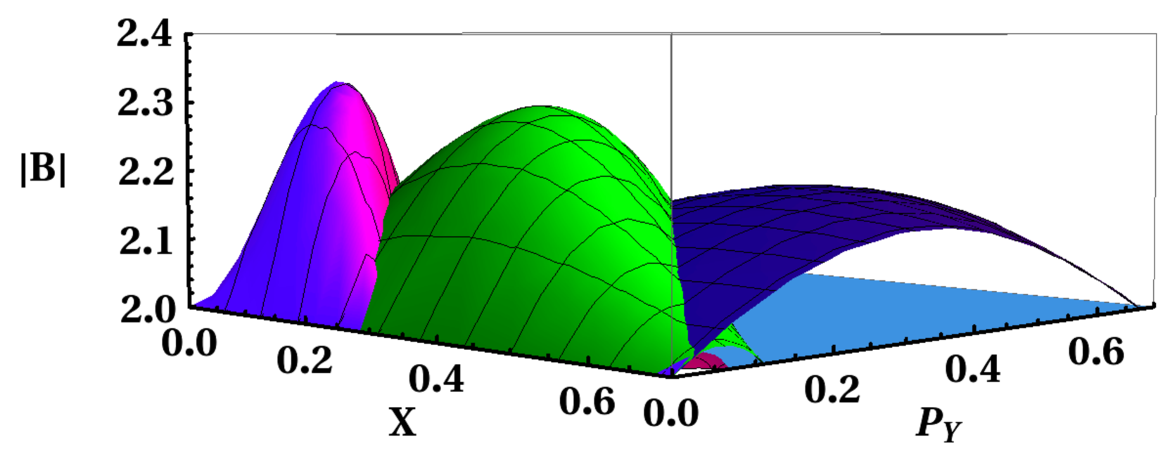
We next repeat the above analysis for higher values of and for the LG field amplitude. We use Eqs.(17) and (19) to calculate the Bell sum. In the Figure 1, we plot against and for three different values of keeping . We find that the violation of the Bell’s inequality increases with higher orbital angular momentum. The increase of Bell violations with is analogous to the enhancement of nonlocality in quantum mechanics for many particle Greenberger-Horne-Zeilinger states or for higher spins mermin , an effect which may also be manifested in physical situations nayak . Here we have been able to demonstrate such an effect within the realm of classical theory.
We would like to note here that for the purpose of experimental realization of the violation of Bell inequalities in classical optical systems with topological singularities, it may be worthwhile to employ techniques for enhancing the Bell violation. This is indeed possible using several approaches, and we would here like to point out two such schemes. First, it has been observed paris that the Bell violation may be further optimized by a more general choice of settings than those used by us in obtaining the Bell sum, i.e.,
| (23) | |||||
Considering the case, and maximizing the Bell violation with respect to the parameters , one obtains the maximum Bell violation, which exceeds the maximum violation obtained through our earlier choice of settings given by Eq.(22), and occurs for the choices of parameters . Similarly, a corresponding increase of the Bell sum occurs for higher values of too. Secondly, another method of obtaining higher violation of Bell inequalities may be through elliptical transformations of LG beams. Such transformations are easily achievable in practice gaussian , viz. a Gaussian elliptical beam of the sort
| (24) |
is observed to increase the Bell violation for the case to .
IV Nonlocal correlations and Bell violations in vortex beams
The violation of the Bell’s inequality obtained above follow from nonvanishing correlations between the two modes of the type , with individually. In quantum mechanics the correlations between two non-commuting observables of a sub-system with those of the other sub-system have rich consequences. In wave optics the wavelength plays a role analogous to the Planck’s constant in quantum mechanics. Thus, nonlocal correlations of the type originate due to the finite and non-vanishing wavelength , resulting in the lack of precision in simultaneous measurement of two observables corresponding to two different modes of light. Note that the above correlations are between separate modes or variables in separate directions, viz., position in the -direction, and momentum in the -direction. Here leads to the limit of geometrical optics, again analogously to the quantum case where gives the classical limit.
Let us now consider the situation where the quadrature phase components of two correlated and spatially separated light fields are measured. The quadrature amplitudes associated with the fields (where, , are the bosonic operators for two different modes, is the frequency, and is a constant incorporating spatial factors taken to be equal for each mode) are given by
| (25) |
where,
| (26) |
and the commutation relations of the bosonic operators are given by . Now, using Eq.(26) the expression for the quadratures can be rewritten as
| (27) |
The correlations between the quadrature amplitudes and are captured by the correlation coefficient, defined as reid ; ou ; tara
| (28) |
where . The correlation is perfect for some values of and , if . Clearly for uncorrelated variables. For the case of LG beams with , the correlation function is given by
| (29) |
Here, the maximum correlation strength occurs for (where is an odd integer). For arbitrary values of it can be shown that the expression for the maximum correlation function is given by
| (30) |
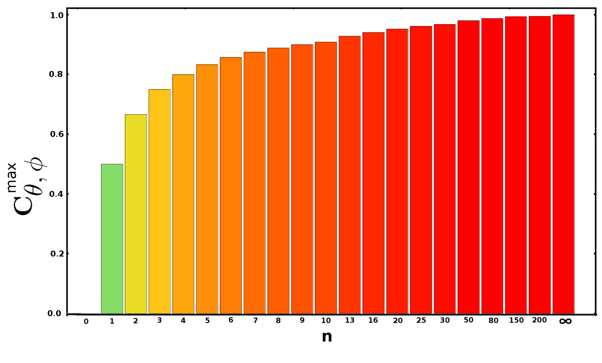
In Fig.2 we provide a plot of the the maximum correlation function for several values of . The strength of the correlations increases with , asymptotically reaching the limit of perfect correlations as becomes very large, as is expected to be the case due to the presence of more and more terms in the Schmidt decomposition of LG beams banerji . This feature thus further corroborates our earlier results of increase in Bell violations for larger orbital angular momentum of LG beams.
V Conclusions
To summarize, in this work we have presented the first study of nonlocal correlations in classical optical beams with topological singularities. These nonlocal correlations between two different light modes are manifested through the violation of a Bell inequality using the Wigner function for this system of classical vortex beams. We need to use the Wigner function as we are dealing with two continuous variables. The magnitude of violation of the Bell inequality is shown to increase with the value of orbital angular momentum of the beam, an effect that is analogous to the enhancement of nonlocality for many particle Greenberger-Horne-Zeilinger states or for higher spins mermin . This feature is further corroborated by the corresponding increase of the quadrature correlation function. Our predicted values of the correlation function as function of the beam parameters should be not difficult to realize experimentally, since production of such vortex beams have been achieved not only in the optical domain fickler ; singh , but recently has also been implemented for electron beams science having far-reaching applications. The feasibility of direct measurement of the two-point correlation function through shear Sagnac interferometry iaconis ; zhang ; singh is a potentially promising avenue for experimental verification of our predicted Bell violation and its enhancement for vortex beams with higher angular momentum. We expect the results of this paper to hold also for other types of beams with no azimuthal symmetry. An example would be Bessel beams bessel of higher order . As emphasized in Section IV, we need nonlocal correlations, i.e., , and beams with no azimuthal symmetry do have this property.
Clearly, the violation of the Bell inequality (18) for classical light fields and the existence of nonlocal correlations (29) bring out totally new statistical features of the optical beams. Traditionally, statistical optics is pursued in terms of the coherence function defined as . Here the brackets refer to the ensemble average. The new features are contained in the quantities defined by (28). The correlations like , give the standard beam characteristics, whereas a correlation like is a correlation between two conjugate variables and can be studied by examining fields in position and momentum spaces. The Wigner function (17) of the LG beams captures this aspect nicely via its dependence on the variable . Clearly, the present work provides a new paradigm to the well developed optical coherence theory.
Acknowledgements: One of us (ASM) thanks Oklahoma State University for the hospitality while this work was done.
References
- (1) J. F. Nye and M. V. Berry, Proc. R. Soc. London Ser. A 165, 336 (1974).
- (2) D. G. Grier, Nature 424, 810 (2003).
- (3) J. H. Lee, et al., Phys. Rev. Lett. 97, 053901 (2006); F. Tamburini et al., New J. Phys. 14, 033001 (2012).
- (4) R. Simon and G. S. Agarwal, J. Opt. Soc. Am. 25, 1313 (2000).
- (5) G. S. Agarwal and J. Banerji, Opt. Lett. 27, 800 (2002).
- (6) G. Molina-Terriza, J. P. Torres, L. Torner, Nature Phys. 3, 305 (2007).
- (7) R. Fickler et al., Science 338, 640 (2012).
- (8) J. Verbeeck, H. Tian and P. Schattschneider, Nature, 467, 301 (2010); B. J. McMorran et al., Science 331, 192 (2011).
- (9) E. Wolf, Phys. Lett. A 312, 263 (2003).
- (10) R. Horodecki, P. Horodecki, M. Horodecki, K. Horodecki, Horodecki, Rev. Mod. Phys. 81, 865 (2009).
- (11) R. J. C. Spreeuw, Found. Phys. 28, 361 (1998); A. Aiello and J. P. Woerdman, Phys. Rev. Lett. 94, 090406 (2005); X-F. Qian and J. H. Eberly, Opt. Lett. 36, 4110 (2011); X-F. Qian, C. J. Broadbent and J. H. Eberly, arxiv:1302.6134.
- (12) B. N. Simon et al, Phys. Rev. Lett. 104, 023901 (2010).
- (13) A. K. Jha, G. S. Agarwal and R. W. Boyd, Phys. Rev. A 84, 063847 (2011).
- (14) J. S. Bell, Physics 1, 195 (1964).
- (15) J.F. Clauser, M.A. Horne, A. Shimony, et al., Phys. Rev. Lett. 23 880 (1969).
- (16) K. H. Kagalwala et al., Nature Photonics 7, 72 (2013).
- (17) D. Bohm, Quantum Theory (Prentice-Hall, Englewood Cliffs, NJ, 1957).
- (18) R. Grobe, K. Rzazewski and J. H. Eberly, J. Phys. B 27, L503 (1994); C. K. Law, I. A. Walmsley and J. H. Eberly, Phys. Rev. Lett. 84, 5304 (2000).
- (19) J. Sperling and V. Vogel, Physica Scripta 83, 045002 (2011).
- (20) J. Sperling and W. Vogel, Phys. Rev. A 79, 042337 (2009).
- (21) B. E. A. Saleh and M. C. Teich, Fundamentals of Photonics, (Wiley, New Jersey, 2007) p 48.
- (22) G. S. Agarwal, Quantum optics (Cambridge University Press, 2013), p 146.
- (23) S. Danakas and P. K. Aravind, Phys. Rev. A 45, 1973 (1992); M. W. Beigersbergen, et al., Opt. Commun. 96, 123 (1993).
- (24) A. Aspect, P. Grangier, and G. Roger, Phys. Rev. Lett. 47, 460 (1981); 49, 91 (1982); A. Aspect, J. Dalibard, and G. Roger, ibid. 49, 1804 (1982).
- (25) K. Banaszek, and K. Wodkiewicz, Phys. Rev. A 58, 4345 (1998); Phys. Rev. Lett. 82, 2009 (1999).
- (26) L. Zhang et al., in Quantum Information with Continuous Variables of Atoms and Light (Imperial College Press, 2007) p 375.
- (27) H. Jeong, W. Son, M. S. Kim, D. Ahn, and C. Brukner, Phys. Rev. A 67, 012106 (2003); S. Olivares and M. G. A. Paris, Phys. Rev. A 70, 032112 (2004).
- (28) L. Zhang et al., Journal of Modern Optics 54, 707 (2007).
- (29) C. Iaconis and I. A. Walmsley, Opt. Lett. 21, 1783 (1996).
- (30) N. D. Mermin, Phys. Rev. Lett. 65, 1838 (1990); S. M. Roy and V. Singh, Phys. Rev. Lett. 67, 2761 (1991); N. Gisin and A. Peres, Phys. Lett. A 162, 15 (1992); D. Home and A. S. Majumdar, Phys. Rev. A 52, 4959 (1995).
- (31) A. S. Majumdar and N. Nayak, Phys. Rev. A 64, 013821 (2001).
- (32) M. A. Bandres and J. C. Gutierrez-Vega, Opt. Express 16, 21087 (2008); N. Verrier et al., JOSA A 25, 1459 (2008).
- (33) M. D. Reid, Phys. Rev. A 40, 913 (1989).
- (34) Z. Y. Ou, S. F. Pereira, H. J. Kimble, and K. C. Peng, Phys. Rev. Lett. 68, 3663 (1992).
- (35) K. Tara and G. S. Agarwal, Phys. Rev. A 50, 2870 (1994).
- (36) R. P. Singh, et al., J. Mod. Opt. 53, 1803 (2006).
- (37) J. Durnin, J. J. Miceli, Jr, and J. H. Eberly, Phys. Rev. Lett. 58, 1499 (1987); V. Garces-Chavez, et al., Nature 419, 145 (2002); F. G. Mitri, Annals of Physics 323, 1604 (2008).