Stability of multi-solitons in the cubic NLS equation

Andres Contreras and Dmitry E. Pelinovsky Department of Mathematics and Statistics, McMaster University, Hamilton ON, Canada, L8S 4K1
Abstract.

We address stability of multi-solitons in the cubic NLS (nonlinear Schrödinger) equation on the line. By using the dressing transformation and the inverse scattering transform methods, we obtain the orbital stability of multi-solitons in the $L^{2}(\mathbb{R})$ space when the initial data is in a weighted $L^{2}(\mathbb{R})$ space.

1. Introduction

We study stability properties of multi-solitons in the cubic NLS (nonlinear Schrödinger) equation

(1.1) $$i\partial_{t}q+\partial_{x}^{2}q+2\left|q\right|^{2}q=0,$$

where $q(x,t):\mathbb{R}\times\mathbb{R}\to\mathbb{C}$. The initial value problem for the cubic NLS equation (1.1) associated with initial data $q|_{t=0}=q_{0}$ is locally well-posed in $L^{2}(\mathbb{R})$ thanks to the result of Tsutsumi based on Stritcharz inequalities [19]. It has a global solution in $L^{2}(\mathbb{R})$ thanks to the conservation of the $L^{2}(\mathbb{R})$ norm in time $t$:

(1.2) $$\|q(\cdot,t)\|_{L^{2}(\mathbb{R})}=\|q_{0}\|_{L^{2}(\mathbb{R})},\quad t\in\mathbb{R}.$$

The cubic NLS equation (1.1) can be studied by methods of the direct and inverse scattering transforms known since the two classical works of Zakharov and Shabat [20, 21]. There exists a vast literature on various applications of the inverse scattering transform methods to the cubic NLS equation (1.1), which we do not intend to overview (see, e.g., the recent book [1, 2]).

Our particular emphasis is on the problem of nonlinear stability of multi-solitons, which are known to exist in the explicit form [20, 21]. Spectral and orbital stability of $n$-solitons in Sobolev space $H^{n}(\mathbb{R})$ was proved by Kapitula [12], based on the classical work of Grillakis, Shatah, and Strauss on stability of $1$-solitons in $H^{1}(\mathbb{R})$ [9].

Functional analytic methods were developed to study interactions of many widely separated solitons in $H^{1}(\mathbb{R})$ for the NLS equation with cubic and higher-order nonlinearities, in particular, by Perelman [17], Rodnianski, Schlag, and Soffer [18], and Martel, Merle, and Tsai [14]. Recent progress along this direction includes the work of Holmer and Zworski [11] on interaction of a soliton with a $\delta$-distribution impurity and the work of Holmer and Lin [10] on interactions of two solitons. Because the inverse scattering transform methods are not used in this literature, the results are usually weaker than those obtained with the inverse scattering transform methods.

New results on stability of $1$-solitons were obtained recently in the context of the cubic NLS equation (1.1) by combining functional analytic methods and the inverse scattering transform. Deift and Park [4] computed long-time asymptotics for the NLS equation with a delta potential to prove asymptotic stability of soliton-defect modes in a weighted $L^{2}(\mathbb{R})$ space and to improve earlier results of Holmer and Zworski [11]. Mizumachi and Pelinovsky [15] proved orbital stability of $1$-solitons in $L^{2}(\mathbb{R})$ improving the standard results of Grillakis, Shatah, and Strauss [9]. Cuccagna and Pelinovsky [3] proved asymptotic stability of $1$-solitons in a weighted $L^{2}(\mathbb{R})$ space by combining the inverse scattering and the steepest descent method, which was earlier developed in a different context by Deift and Zhou [5, 6, 24].

In this paper, we would like to extend the results of [3, 4, 15] to multi-solitons of the cubic NLS equation (1.1) by combining the inverse scattering transform methods and the dressing transformation, which was developed by Zakharov and Shabat long ago [22, 23] (see, e.g., Chapter 3 in book [16]).

We denote by $L^{2,s}(\mathbb{R})$ the weighted $L^{2}(\mathbb{R})$ space with the norm

(1.3) $$\|u\|_{L^{2,s}(\mathbb{R})}:=\|\langle x\rangle^{s}u\|_{L^{2}(\mathbb{R})},\quad\langle x\rangle:=\sqrt{1+x^{2}}.$$

The following theorem gives the main result of this article.

Theorem 1.1.

Let $q^{S}$ be a $n$-soliton solution of the cubic NLS equation (1.1) with real parameters $\{\xi_{j},\eta_{j},x_{j},\theta_{j}\}_{j=1}^{n}$ such that pairs $(\xi_{j},\eta_{j})$ are all distinct. There exist positive constants $\epsilon_{0}$ and $C$ such that if $q_{0}\in L^{2,s}(\mathbb{R})$ for any $s>\frac{1}{2}$ and if

(1.4) $$\epsilon:=\|q_{0}-q^{S}(\cdot,0)\|_{L^{2,s}(\mathbb{R})}<\epsilon_{0}$$

then there exist a solution $q$ of the cubic NLS equation (1.1) with $q|_{t=0}=q_{0}$ and an $n$-soliton solution $q^{S^{\prime}}$ with real parameters $\{{\xi}^{\prime}_{j},{\eta}^{\prime}_{j},{x}^{\prime}_{j},{\theta}^{\prime}_{j}\}_{j=1}^{n}$ such that

(1.5) $$\max_{1\leq j\leq n}\left|({\xi}^{\prime}_{j},{\eta}^{\prime}_{j},{x}^{\prime}_{j},{\theta}^{\prime}_{j})-(\xi_{j},\eta_{j},x_{j},\theta_{j})\right|\leq C\epsilon$$

and

(1.6) $$\|q(\cdot,t)-q^{S^{\prime}}(\cdot,t)\|_{L^{2}(\mathbb{R})}\leq C\epsilon,\quad t\in\mathbb{R}.$$
Remark 1.2.

The orbital stability result (1.6) is not expected in the $L^{2,s}(\mathbb{R})$ norm for $s>0$ because, in a general situation, the variance of the solution $\|xq\|_{L^{2}(\mathbb{R})}$ grows linearly in time $t$, according to the cubic NLS equation (1.1).

For $n=1$, the $L^{2}(\mathbb{R})$ orbital stability result of Theorem 1.6 was proved by Mizumachi and Pelinovsky [15] without the requirement that the initial data is close to the $1$-soliton in the weighted $L^{2}(\mathbb{R})$ space (1.4). Without this requirement, the initial data can support more than one soliton in the long-time asymptotics, but the additional solitons have small $L^{2}(\mathbb{R})$ norm and are included in the residual terms of the $L^{2}(\mathbb{R})$ orbital stability result (1.6).

At the same time, a stronger result on the asymptotic stability of $1$-solitons was proved by Cuccagna and Pelinovsky [3] under the requirement (1.4) with the decay of the $L^{\infty}(\mathbb{R})$ norm of the residual term in time:

(1.7) $$\|q(\cdot,t)-q^{S^{\prime}}(\cdot,t)\|_{L^{\infty}(\mathbb{R})}\leq C\epsilon t^{-1/2},\quad\mbox{\rm as}\quad t\to\infty.$$

We believe that both the orbital stability if $q_{0}\in L^{2}(\mathbb{R})$ and the asymptotic stability if $q_{0}\in L^{2,s}(\mathbb{R})$ with $s>\frac{1}{2}$ hold for $n$ solitons but the proofs of these two refinements of Theorem 1.6 would require considerable lengthening of the present work at the possible expense of obscuring the main argument. Note that a similar constraint on the initial data to enable the inverse scattering transform methods is used by Gerard and Zhang [7] to prove the $L^{\infty}(\mathbb{R})$ orbital stability of black solitons in the cubic defocussing NLS equation.

For $n=2$, the result of Theorem 1.6 provides orbital stability of the class of $2$-solitons in the cubic NLS equation (1.1). Note that interactions of widely separated two solitons in this equation was recently considered by Holmer and Lin [10] using an effective dynamical equation that describes the solitons dynamics for large but finite time. Depending on the parameters $(\xi_{1},\xi_{2},\eta_{1},\eta_{2})$, the two solitons collide and scatter with different velocities but may also form a bound state (a time-oscillating space-localized breather). Although Theorem 1.6 provides orbital stability of the entire family of $2$-solitons, this result does not exclude the phenomenon of instability of the $2$-soliton breather. Indeed, if the breather corresponds to the constraint $\xi_{1}=\xi_{2}$, whereas the initial condition yields $\xi_{1}^{\prime}\neq\xi_{2}^{\prime}$, the time-oscillating breather is destroyed by the initial perturbation and transforms into two solitons moving with different velocities.

The paper is organized as follows. Section 2 gives details of the dressing transformation, which enables us to construct $n$-solitons from the trivial zero solution of the cubic NLS equation (1.1). Section 3 describes the time evolution for the dressing transformation. The exact $n$-solitons are constructed in Section 4. Section 5 is devoted to analysis of the mapping between the $L^{2}$-neighborhood of the zero solution and the $L^{2}$-neighborhood of the $n$-solitons: the mapping is one-to-one but it is not onto, unless the constraints on soliton parameters are imposed. Instead of adding constraints, we determine in Section 6 parameters of the $n$-soliton $q^{S^{\prime}}$ based on the inverse scattering transform methods, which are enabled by adding the requirement (1.4) on the initial data $q_{0}$. All together, these arguments will complete the proof of orbital stability of $n$-solitons in $L^{2}(\mathbb{R})$.

Acknowledgements: A.C. is supported by the postdoctoral fellowship at McMaster University. D.P. is supported in part by the NSERC Discovery grant. The authors are indebted to S. Cuccagna for bringing this problem up and for critical remarks during the preparation of this manuscript.

2. Dressing transformation

We use the dressing method of Zakharov and Shabat [22, 23] to map a neighborhood of the zero solution to a neighborhood of a multi-soliton in the cubic NLS equation (1.1). The dressing method relies on the existence of the Lax operator pair

(2.1) $$\left\{\begin{array}[]{l}\partial_{x}\psi=-iz\sigma_{3}\psi+Q(q)\psi,\\ \partial_{t}\psi=i(|q|^{2}-2z^{2})\sigma_{3}\psi+2zQ(q)\psi-iQ(\partial_{x}q)\sigma_{3}\psi,\end{array}\right.$$

where $\psi(x,t):\mathbb{R}\times\mathbb{R}\to{\mathbb{C}}^{2}$ and

$$Q(q):=\begin{pmatrix}0&q\\ -\overline{q}&0\end{pmatrix},\quad\sigma_{3}:=\begin{pmatrix}1&0\\ 0&-1\end{pmatrix}.$$

The compatibility condition $\psi_{xt}=\psi_{tx}$ for a classical solution $\psi\in C^{2}(\mathbb{R}\times\mathbb{R},\mathbb{C}^{2})$ of the Lax system (2.1) with constant spectral parameter $z$ is equivalent to the requirement that $q(x,t)$ is a classical solution of the NLS equation (1.1), that is, $q$ is $C^{1}$ in $t$ and $C^{2}$ in $x$ for all $(x,t)\in\mathbb{R}\times\mathbb{R}$.

Let $\Phi(x,t,z)$ be a fundamental matrix solution of the system (2.1) such that $\Phi(0,t,z)=I$, where $I$ is a $2\times 2$ identity matrix. In what follows, we will only consider the first part of the system (2.1) and will set $\phi(x,z):=\Phi(x,0,z)$. The time evolution will be added in the next section, according to the standard analysis.

We define a fundamental matrix solution $\phi(x,z):\mathbb{R}\times\mathbb{C}\to\mathbb{M}^{2\times 2}$ from the system of differential equations:

(2.2) $$\left\{\begin{array}[]{l}\partial_{x}\phi=U(x,z)\phi,\\ \phi|_{x=0}=I,\end{array}\right.\quad U(x,z):=-iz\sigma_{3}+Q(q).$$

Since $U^{+}=-U$, where $U^{+}=\bar{U}^{T}$, the fundamental matrix is inverted by the following elementary result.

Proposition 2.1.

Let $\phi$ be a fundamental matrix solution of the system (2.2). Then, $\phi$ is invertible and $\phi^{-1}(x,z)=\phi^{+}(x,z)$.

Proof.

We verify that

$$\partial_{x}\left[\phi^{+}(x,z)\phi(x,z)\right]=\phi^{+}(x,z)U^{+}(x,z)\phi(x,z)+\phi^{+}(x,z)U(x,z)\phi(x,z)=0,$$

so that $\phi^{+}(x,z)\phi(x,z)$ is constant in $x$ and equals to $I$ because $\phi^{+}(0,z)\phi(0,z)=I$. A similar computation holds for $\phi(x,z)\phi^{+}(x,z)$, hence $\phi^{+}(x,z)$ is the inverse for $\phi(x,z)$. ∎

Let $\phi_{0}$ denote the fundamental matrix solution of the system (2.2) for the potential $q_{0}$. In what follows, $q_{0}$ is not related to the initial data in Theorem 1.6 but denotes another (simpler) solution of the cubic NLS equation (1.1). Let us define the matrix function $\phi$ by the dressing transformation formula:

(2.3) $$\phi(x,z):=\chi(x,z)\phi_{0}(x,z),\quad\chi(x,z)=I+\sum_{k=1}^{n}\frac{ir_{k}(x)\otimes\bar{s}_{k}(x)}{z-z_{k}},$$

where for each $k$, ${\rm Im}(z_{k})>0$, $r_{k}(x),s_{k}(x):\mathbb{R}\to\mathbb{C}^{2}$ are to be defined, and $\otimes$ denotes an outer product of vectors in $\mathbb{C}^{2}$ (without complex conjugation). The factor $i$ is used in the sum for convenience. The following result summarizes the dressing method of Zakharov and Shabat [22, 23]. For convenience of readers, we give a precise proof of the dressing transformation.

Proposition 2.2.

Assume $q_{0}\in C(\mathbb{R})$ and define the set $\{s_{k}\}_{k=1}^{n}$ from classical solutions of the Zakharov–Shabat (ZS) system

(2.4) $$\partial_{x}s_{k}=-i\bar{z}_{k}\sigma_{3}s_{k}+Q(q_{0})s_{k},\quad 1\leq k\leq n,$$

such that the Gramian-type matrix with entries

(2.5) $$M_{k,j}:=\frac{-i}{\bar{z}_{k}-z_{j}}\langle s_{j},s_{k}\rangle,\quad 1\leq k,j\leq n$$

is invertible. Let the set $\{r_{k}\}_{k=1}^{n}$ be defined from the set $\{s_{k}\}_{k=1}^{n}$ by unique solution of the linear system

(2.6) $$is_{k}=\sum_{j=1}^{n}\frac{\langle s_{j},s_{k}\rangle}{\bar{z}_{k}-z_{j}}r_{j},\quad 1\leq k\leq n,$$

with the inverse

(2.7) $$ir_{k}=\sum_{j=1}^{n}\frac{\langle r_{j},r_{k}\rangle}{\bar{z}_{j}-z_{k}}s_{j},\quad 1\leq k\leq n,$$

where $\langle u,v\rangle:=\bar{u}_{1}v_{1}+\bar{u}_{2}v_{2}$ is the dot product between vectors in ${\mathbb{C}}^{2}$. Then, the dressing transformation (2.3) is invertible with the inverse

(2.8) $$\phi^{-1}(x,z)=\phi_{0}^{+}(x,z)\chi^{+}(x,z),\quad\chi^{+}(x,z)=I-\sum_{k=1}^{n}\frac{is_{k}(x)\otimes\bar{r}_{k}(x)}{z-\bar{z}_{k}},$$

and $\phi$ is a solution of the system $\partial_{x}\phi=U(x,z)\phi$ for the potential $q$, which is related to the potential $q_{0}$ by the transformation formula

(2.9) $$Q(q)=Q(q_{0})+\sum_{k=1}^{n}r_{k}\otimes\bar{s}_{k}\sigma_{3}-\sigma_{3}s_{k}\otimes\bar{r}_{k}.$$

In addition, the set $\{r_{k}\}_{k=1}^{n}$ satisfies the ZS system

(2.10) $$\partial_{x}r_{k}=-iz_{k}\sigma_{3}r_{k}+Q(q)r_{k},\quad 1\leq k\leq n,$$

associated with the same potential $q$.

Proof.

First, we check that

$$\chi^{+}(x,z)\chi(x,z)=\chi(x,z)\chi^{+}(x,z)=I,$$

which yields

$$\phi^{+}(x,z)\phi(x,z)=\phi(x,z)\phi^{+}(x,z)=I.$$

We use the partial fraction

$$\frac{1}{(z-\bar{z}_{j})(z-z_{k})}=\frac{1}{\bar{z}_{j}-z_{k}}\left[\frac{1}{z-\bar{z}_{j}}-\frac{1}{z-z_{k}}\right].$$

Then $\chi(x,z)\chi^{+}(x,z)=I$ is equivalent to the system

$$ir_{k}\otimes\bar{s}_{k}=\sum_{j=1}^{n}\frac{(r_{k}\otimes\bar{s}_{k})\;(s_{j}\otimes\bar{r}_{j})}{\bar{z}_{j}-z_{k}},$$

which yields the system (2.6) after projection to $r_{k}$ from the left.

Now, since $\chi(x,z)$ is a square $n\times n$ matrix and $\chi(x,z)\chi^{+}(x,z)=I$, then $|\det(\chi(x,z))|=1$ and therefore, $\chi(x,z)$ is invertible with $\chi^{-1}(x,z)=\chi^{+}(x,z)$. On the other hand, $\chi^{+}(x,z)\chi(x,z)=I$ is equivalent to the system

$$ir_{k}\otimes\bar{s}_{k}=\sum_{j=1}^{n}\frac{(s_{j}\otimes\bar{r}_{j})\;(r_{k}\otimes\bar{s}_{k})}{\bar{z}_{j}-z_{k}},$$

which yields the system (2.7) after projection to $s_{k}$ from the right. Therefore, the system (2.7) is inverse to the system (2.6)). Note that all vectors in the sets $\{s_{k}\}_{k=1}^{n}$ and $\{r_{k}\}_{k=1}^{n}$ are nonzero because the matrix $M$ in (2.5) is invertible.

Next, we confirm that the set $\{r_{k}\}_{k=1}^{n}$, which is determined by the linear system (2.6), satisfies the ZS system (2.10) with the potential $q$ if the set $\{s_{k}\}_{k=1}^{n}$ satisfies the ZS system (2.4) with the potential $q_{0}$, where $q$ and $q_{0}$ are related by the transformation formula (2.9). Differentiating the linear system (2.6) in $x$ and substituting (2.4), we obtain

$\displaystyle\bar{z}_{k}\sigma_{3}s_{k}+iQ(q_{0})s_{k}=-i\sum_{j=1}^{n}\langle\sigma_{3}s_{j},s_{k}\rangle r_{j}+\sum_{j=1}^{n}\frac{\langle s_{j},s_{k}\rangle}{\bar{z}_{k}-z_{j}}\partial_{x}r_{j}.$

Using the transformation formula (2.9) and the inverse linear system (2.7), we rewrite this equation as follows:

$\displaystyle\sum_{j=1}^{n}\frac{\langle s_{j},s_{k}\rangle}{\bar{z}_{k}-z_{j}}\partial_{x}r_{j}$ $\displaystyle=$ $\displaystyle\bar{z}_{k}\sigma_{3}s_{k}+\sum_{j=1}^{n}\frac{\langle s_{j},s_{k}\rangle}{\bar{z}_{k}-z_{j}}Q(q)r_{j}+i\sigma_{3}\sum_{j=1}^{n}\langle r_{j},s_{k}\rangle s_{j}$
$\displaystyle=$ $\displaystyle\bar{z}_{k}\sigma_{3}s_{k}+\sum_{j=1}^{n}\frac{\langle s_{j},s_{k}\rangle}{\bar{z}_{k}-z_{j}}Q(q)r_{j}+i\sigma_{3}\sum_{j=1}^{n}\langle s_{j},s_{k}\rangle r_{j},$

where the following transformation was used:

$\displaystyle i\sum_{m=1}^{n}\langle r_{m},s_{k}\rangle s_{m}$ $\displaystyle=$ $\displaystyle\sum_{m=1}^{n}\sum_{j=1}^{n}\frac{\langle r_{m},r_{j}\rangle\langle s_{j},s_{k}\rangle}{\bar{z}_{m}-z_{j}}s_{m}$
$\displaystyle=$ $\displaystyle\sum_{j=1}^{n}\langle s_{j},s_{k}\rangle\sum_{m=1}^{n}\frac{\langle r_{m},r_{j}\rangle}{\bar{z}_{m}-z_{j}}s_{m}$
$\displaystyle=$ $\displaystyle i\sum_{j=1}^{n}\langle s_{j},s_{k}\rangle r_{j}.$

Using the linear system (2.6) again, we obtain

$\displaystyle\sum_{j=1}^{n}\frac{\langle s_{j},s_{k}\rangle}{\bar{z}_{k}-z_{j}}\left[\partial_{x}r_{j}+iz_{j}\sigma_{3}r_{j}-Q(q)r_{j}\right]=0,$

which yields the ZS system (2.10), because the matrix $M$ in (2.5) is invertible.

We shall now verify that $\phi(x,z)$ is a solution of the system $\partial_{x}\phi=U\phi$ from the condition

(2.12) $$U(x,z)=\partial_{x}\phi(x,z)\phi^{-1}(x,z)=\left[\partial_{x}\chi(x,z)+\chi(x,z)U_{0}(x,z)\right]\chi^{+}(x,z),$$

where $U_{0}(x,z)=\partial_{x}\phi_{0}(x,z)\phi_{0}^{-1}(x,z)$. By using the partial fraction decompositions, we shall first remove the residue terms at simple poles of equation (2.12).

The residue terms at $\mathcal{O}\left(\frac{1}{z-z_{k}}\right)$ are removed from equation (2.12) if

$\displaystyle\left[i\partial_{x}\left(r_{k}\otimes\bar{s}_{k}\right)+z_{k}r_{k}\otimes\bar{s}_{k}\sigma_{3}+ir_{k}\otimes\bar{s}_{k}Q(q_{0})\right]\left[I-i\sum_{j=1}^{n}\frac{s_{j}\otimes\bar{r}_{j}}{z_{k}-\bar{z}_{j}}\right]=0.$

Because of the linear system (2.6), this equation simplifies to the form

$\displaystyle r_{k}\otimes\left[i\partial_{x}\bar{s}_{k}+z_{k}\bar{s}_{k}\sigma_{3}+i\bar{s}_{k}Q(q_{0})\right]\left[I-i\sum_{j=1}^{n}\frac{s_{j}\otimes\bar{r}_{j}}{z_{k}-\bar{z}_{j}}\right]=0.$

Projection to $r_{k}$ from the left (assuming $r_{k}$ is nonzero) and Hermite conjugation with the help of equation $Q^{+}(q_{0})=-Q(q_{0})$ yields the new equation

$\displaystyle\left[I+i\sum_{j=1}^{n}\frac{r_{j}\otimes\bar{s}_{j}}{\bar{z}_{k}-z_{j}}\right]\left[-i\partial_{x}s_{k}+\bar{z}_{k}\sigma_{3}s_{k}+iQ(q_{0})s_{k}\right]=0,$

which is satisfied if $s_{k}$ is a nonzero solution of the ZS system (2.4). Note that the operator on the left has a nontrivial kernel, hence the ZS system (2.4) is only a particular solution of the constraint.

Next, the residue terms at $\mathcal{O}\left(\frac{1}{z-\bar{z}_{j}}\right)$ are removed from equation (2.12) if

$\displaystyle\left[\partial_{x}\left(\sum_{k=1}^{n}\frac{r_{k}\otimes\bar{s}_{k}}{\bar{z}_{j}-z_{k}}\right)-\bar{z}_{j}\sigma_{3}-iQ(q_{0})-i\bar{z}_{j}\sum_{k=1}^{n}\frac{r_{k}\otimes\bar{s}_{k}}{\bar{z}_{j}-z_{k}}\sigma_{3}+\sum_{k=1}^{n}\frac{r_{k}\otimes\bar{s}_{k}}{\bar{z}_{j}-z_{k}}Q(q_{0})\right]s_{j}\otimes\bar{r}_{j}=0.$

Projection to $r_{j}$ from the right yields the new equation

$\displaystyle\left[\partial_{x}\left(\sum_{k=1}^{n}\frac{r_{k}\otimes\bar{s}_{k}}{\bar{z}_{j}-z_{k}}\right)-\bar{z}_{j}\sigma_{3}-iQ(q_{0})-i\bar{z}_{j}\sum_{k=1}^{n}\frac{r_{k}\otimes\bar{s}_{k}}{\bar{z}_{j}-z_{k}}\sigma_{3}+\sum_{k=1}^{n}\frac{r_{k}\otimes\bar{s}_{k}}{\bar{z}_{j}-z_{k}}Q(q_{0})\right]s_{j}=0.$

If $s_{k}$ is a solution of the ZS system (2.4), then this equation reduces further to the form

$\displaystyle\left[\sum_{k=1}^{n}\frac{(\partial_{x}r_{k})\otimes\bar{s}_{k}}{\bar{z}_{j}-z_{k}}-\bar{z}_{j}\sigma_{3}-iQ(q_{0})-i\sum_{k=1}^{n}r_{k}\otimes\bar{s}_{k}\sigma_{3}\right]s_{j}=0,$

where the derivative in $x$ applies now to $r_{k}$ only. This equation is rewritten with the help of the reconstruction formula (2.9) in the form

$\displaystyle\sum_{k=1}^{n}\frac{\langle s_{k},s_{j}\rangle}{\bar{z}_{j}-z_{k}}\partial_{x}r_{k}-\bar{z}_{j}\sigma_{3}s_{j}-iQ(q)s_{j}-i\sigma_{3}\sum_{m=1}^{n}\langle r_{m},s_{j}\rangle s_{m}=0.$

Substituting transformation (2) to the previous equation and using the linear system (2.6), we derive

$\displaystyle\sum_{k=1}^{n}\frac{\langle s_{k},s_{j}\rangle}{\bar{z}_{j}-z_{k}}\left[\partial_{x}r_{k}-Q(q)r_{k}+iz_{k}\sigma_{3}r_{k}\right]-\bar{z}_{j}\sigma_{3}s_{j}-i\bar{z}_{j}\sigma_{3}\sum_{k=1}^{n}\frac{\langle s_{k},s_{j}\rangle}{\bar{z}_{j}-z_{k}}r_{k}=0.$

The last two terms cancel out thanks to the linear system (2.6). As a result, the equation is satisfied if $r_{k}$ is a solution of the ZS system (2.10).

Now, since all the residue terms are removed from equation (2.12), this equation reduces a single equation, which is nothing but the reconstruction formula (2.9). ∎

Remark 2.3.

Note that $\phi$ given by (2.3) is not the fundamental matrix solution of the system (2.2) because $\phi|_{x=0}=I$ is not satisfied. However, if we define

$$\phi(x,z):=\chi^{+}(0,z)\chi(x,z)\phi_{0}(x,z),$$

then this $\phi$ is the fundamental matrix solution of the system (2.2).

For $1$-soliton solutions with $n=1$, the result of Proposition 2.2 can be simplified as follows. Let $q_{0}=0$, $z_{1}=\xi_{1}+i\eta_{1}$ with $\eta_{1}>0$, and let $s_{1}=(\mathfrak{b}_{1},\mathfrak{b}_{2})$ be a solution of the ZS system (2.4) with $q_{0}=0$, or explicitly:

(2.13) $$\left\{\begin{array}[]{l}\partial_{x}\mathfrak{b}_{1}=-(\eta_{1}+i\xi_{1})\mathfrak{b}_{1},\\ \partial_{x}\mathfrak{b}_{2}=(\eta_{1}+i\xi_{1})\mathfrak{b}_{2}.\end{array}\right.$$

Then, $r_{1}=(\mathfrak{a}_{1},\mathfrak{a}_{2})$ is found from the linear system (2.6) in the closed form:

(2.14) $$\left[\begin{array}[]{c}\mathfrak{a}_{1}\\ \mathfrak{a}_{2}\end{array}\right]=\frac{2\eta_{1}}{|\mathfrak{b}_{1}|^{2}+|\mathfrak{b}_{2}|^{2}}\left[\begin{array}[]{c}\mathfrak{b}_{1}\\ \mathfrak{b}_{2}\end{array}\right].$$

Note that $r_{1}$ is an eigenfunction for an isolated eigenvalue $z_{1}=\xi_{1}+i\eta_{1}$ of the ZS system (2.10) associated with the $1$-soliton. The transformation formula (2.9) yields $1$-soliton:

(2.15) $$q=-\mathfrak{a}_{1}\bar{\mathfrak{b}}_{2}-\bar{\mathfrak{a}}_{2}\mathfrak{b}_{1}=\frac{-4\eta_{1}\mathfrak{b}_{1}\bar{\mathfrak{b}}_{2}}{|\mathfrak{b}_{1}|^{2}+|\mathfrak{b}_{2}|^{2}}.$$

Setting a general solution of the ZS system (2.13) in the form

$$\left\{\begin{array}[]{c}\mathfrak{b}_{1}=e^{-(\eta_{1}+i\xi_{1})(x-x_{0})+i\theta},\\ \mathfrak{b}_{2}=-e^{(\eta_{1}+i\xi_{1})(x-x_{0})-i\theta},\end{array}\right.$$

where $x_{0},\theta\in\mathbb{R}$ are arbitrary parameters, we obtain from (2.14) and (2.15) the $1$-soliton with four arbitrary parameters:

(2.16) $$q=2\eta_{1}{\rm sech}(2\eta_{1}(x-x_{0}))e^{2i\theta-2i\xi_{1}(x-x_{0})}.$$

Note that parameters $(x_{0},\theta)$ can be set to zero by using the translational and gauge transformations of the cubic NLS equation (1.1), parameter $\xi_{1}$ can be set to zero by using the Galileo transformation, and parameter $\eta_{1}$ can be fixed at any positive number because of the scaling transformation.

Remark 2.4.

Note that the result of the dressing method is different from the result of the auto-Backlund transformation used in recent papers [3, 4, 15], where the vector $(\mathfrak{b}_{1},\mathfrak{b}_{2})$ in the soliton reconstruction formula (2.15) was defined in terms of the solution of the spectral system (2.4) with $z_{1}$ instead of $\bar{z}_{1}$.

3. Time evolution of the dressing transformation

Before looking at the time evolution of the dressing transformations, let us give an explicit representation of the dressing transformation with the help of matrix algebra.

Let the set $\{s_{k}\}_{k=1}^{n}$ be defined by the solutions of the Zakharov–Shabat system (2.4) such that the Gramian-type matrix $M$ in (2.5) is invertible. Vectors $\{r_{k}\}_{k=1}^{n}$ are uniquely defined by the linear system (2.6).

Let $D:=\det(M)$ and $D_{k,j}$ be the co-factor of the element $M_{k,j}$. Because $M$ is invertible, we have $D\neq 0$. A unique solution of the linear system (2.6) can be expressed in the explicit form

(3.1) $$r_{k}=\sum_{j=1}^{n}\frac{D_{j,k}}{D}s_{j}.$$

Note that matrix $M$ is Hermitian and hence, $D_{j,k}=\bar{D}_{k,j}$. Under this constraint, the transformation formula (2.9) yields

$$Q(q)-Q(q_{0})=\sum_{k=1}^{n}r_{k}\otimes\bar{s}_{k}\sigma_{3}-\sigma_{3}s_{k}\otimes\bar{r}_{k}=\sum_{k=1}^{n}\left(\begin{array}[]{cc}r_{k,1}\bar{s}_{k,1}-\bar{r}_{k,1}s_{k,1}&-r_{k,1}\bar{s}_{k,2}-\bar{r}_{k,2}s_{k,1}\\ r_{k,2}\bar{s}_{k,1}+\bar{r}_{k,1}s_{k,2}&-r_{k,2}\bar{s}_{k,2}+\bar{r}_{k,2}s_{k,2}\end{array}\right),$$

where the diagonal entries are zeros and the off-diagonal entries yield the transformation formula

(3.2) $$q-q_{0}=-\sum_{k=1}^{n}\sum_{j=1}^{n}\left(\frac{D_{j,k}}{D}s_{j,1}\bar{s}_{k,2}+\frac{\bar{D}_{j,k}}{D}s_{k,1}\bar{s}_{j,2}\right)=-\frac{2}{D}\sum_{k=1}^{n}\sum_{j=1}^{n}D_{j,k}s_{j,1}\bar{s}_{k,2}.$$

The time-dependent part of the Lax operator (2.1) can be included into consideration thanks to the compatibility between the two linear equations and the independence of the spectral parameter $z$ from variables $(x,t)$, under the condition that $q$ is a classical solution of the cubic NLS equation (1.1). Therefore, we consider the time-dependent system

(3.3) $$\partial_{t}\phi=V(x,t,z)\phi,\quad V(x,t,z):=i(|q|^{2}-2z^{2})\sigma_{3}+2zQ(q)-iQ(\partial_{x}q)\sigma_{3}.$$

We assume that $q_{0}$ is a classical solution of the cubic NLS equation (1.1) and $\phi_{0}$ is a matrix solution of the system (3.3) for the potential $q_{0}$. Then, we define the matrix function $\phi$ by the same dressing transformation formula (2.3). The following result gives a time-dependent analogue of Proposition 2.2.

Proposition 3.1.

In addition to conditions of Proposition 2.2, assume that $q_{0}$ is a classical solution of the cubic NLS equation (1.1) and the set $\{s_{k}\}_{k=1}^{n}$ yields a classical solution of the time-evolution part of the Lax operator pair

(3.4) $$\partial_{t}s_{k}=i(|q_{0}|^{2}-2\bar{z}_{k}^{2})\sigma_{3}s_{k}+2\bar{z}_{k}Q(q_{0})s_{k}-iQ(\partial_{x}q_{0})\sigma_{3}s_{k},\quad 1\leq k\leq n.$$

Let $\phi$ be defined by the dressing transformation (2.3), the set $\{r_{k}\}_{k=1}^{n}$ be defined by the linear system (2.6), and $q$ be defined by the transformation formula (2.9). Then, $\phi$ is a solution of the system (3.3) for the potential $q$, $\{r_{k}\}_{k=1}^{n}$ is a solution of the time-evolution part of the Lax operator pair

(3.5) $$\partial_{t}r_{k}=i(|q|^{2}-2z_{k}^{2})\sigma_{3}r_{k}+2z_{k}Q(q)r_{k}-iQ(\partial_{x}q)\sigma_{3}r_{k},\quad 1\leq k\leq n,$$

and $q$ is a classical solution of the cubic NLS equation (1.1). In addition to the transformation formula (2.9), $q$ and $q_{0}$ are related by

(3.6) $$|q|^{2}=|q_{0}|^{2}+\partial_{x}^{2}\log(D),$$

where $D:=\det(M)$ and $M$ is given by the Gramian-type matrix (2.5).

Proof.

We shall prove that the linear system (2.6) and equations (3.4) yield equations (3.5). The transformation formula (3.6) will be discovered naturally in this reduction. The fact that $\phi$ is a solution of the system (3.3) for the potential $q$ follows from this reduction and is proved similarly to Proposition 2.2. Finally, $q$ is sufficiently smooth as it is defined by the transformation formula (2.9). As $q$ is a compatibility condition between systems (2.10) and (3.5), $q$ becomes a classical solution of the cubic NLS equation (1.1).

To derive equations (3.5), we differentiate the linear system (2.6) and substitute equations (3.4) to obtain

$\displaystyle(2\bar{z}_{k}^{2}-|q_{0}|^{2})\sigma_{3}s_{k}+2i\bar{z}_{k}Q(q_{0})s_{k}+iQ(\partial_{x}q_{0})\sigma_{3}s_{k}$
$\displaystyle=-2i\sum_{j=1}^{n}(\bar{z}_{k}+z_{j})\langle\sigma_{3}s_{j},s_{k}\rangle r_{j}-2\sum_{j=1}^{n}\langle Q(q_{0})s_{j},s_{k}\rangle r_{j}+\sum_{j=1}^{n}\frac{\langle s_{j},s_{k}\rangle}{\bar{z}_{k}-z_{j}}\partial_{t}r_{j}.$

This can be written as

$\displaystyle\sum_{j=1}^{n}\frac{\langle s_{j},s_{k}\rangle}{\bar{z}_{k}-z_{j}}\left[\partial_{t}r_{j}-i(|q|^{2}-2z_{k}^{2})\sigma_{3}r_{k}-2z_{k}Q(q)r_{k}+iQ(\partial_{x}q)\sigma_{3}r_{k}\right]=G_{k},$

where

$\displaystyle G_{k}$ $\displaystyle:=$ $\displaystyle(2\bar{z}_{k}^{2}-|q_{0}|^{2})\sigma_{3}s_{k}+2i\bar{z}_{k}Q(q_{0})s_{k}+iQ(\partial_{x}q_{0})\sigma_{3}s_{k}+2i\sum_{j=1}^{n}(\bar{z}_{k}+z_{j})\langle\sigma_{3}s_{j},s_{k}\rangle r_{j}$
$\displaystyle+2\sum_{j=1}^{n}\langle Q(q_{0})s_{j},s_{k}\rangle r_{j}+i\sum_{j=1}^{n}\frac{\langle s_{j},s_{k}\rangle}{\bar{z}_{k}-z_{j}}(|q|^{2}-2z_{j}^{2})\sigma_{3}r_{j}$
$\displaystyle+2\sum_{j=1}^{n}\frac{\langle s_{j},s_{k}\rangle}{\bar{z}_{k}-z_{j}}z_{j}Q(q)r_{j}-i\sum_{j=1}^{n}\frac{\langle s_{j},s_{k}\rangle}{\bar{z}_{k}-z_{j}}Q(\partial_{x}q)\sigma_{3}r_{j}.$

If $G_{k}=0$, then invertibility of the matrix $M$ in (2.5) implies validity of equations (3.5). To show that $G_{k}=0$, we use the linear system (2.6) and rewrite

$\displaystyle G_{k}$ $\displaystyle=$ $\displaystyle(|q|^{2}-|q_{0}|^{2})\sigma_{3}s_{k}+2i\bar{z}_{k}\left[Q(q_{0})-Q(q)\right]s_{k}+\left[Q(\partial_{x}q_{0})-Q(\partial_{x}q)\right]\sigma_{3}s_{k}$
$\displaystyle+2i\sum_{j=1}^{n}(\bar{z}_{k}+z_{j})\langle\sigma_{3}s_{j},s_{k}\rangle r_{j}+2\sum_{j=1}^{n}\langle Q(q_{0})s_{j},s_{k}\rangle r_{j}$
$\displaystyle-2i\sum_{j=1}^{n}(\bar{z}_{k}+z_{j})\langle s_{j},s_{k}\rangle\sigma_{3}r_{j}+2\sum_{j=1}^{n}\langle s_{j},s_{k}\rangle Q(q)r_{j}.$

We can now use the transformation formula (2.9) and its derivative version in the following form:

$$Q(\partial_{x}q)-Q(\partial_{x}q_{0})=2\sum_{j=1}^{n}(\partial_{x}r_{j})\otimes\bar{s}_{j}\sigma_{3}+r_{j}\otimes(\partial_{x}\bar{s}_{j})\sigma_{3}-\partial_{x}R,$$

where

$$R:=\sum_{j=1}^{n}r_{j}\otimes\bar{s}_{j}\sigma_{3}+\sigma_{3}s_{j}\otimes\bar{r}_{j}=\sum_{j=1}^{n}\left(\begin{array}[]{cc}r_{j,1}\bar{s}_{j,1}+\bar{r}_{j,1}s_{j,1}&-r_{j,1}\bar{s}_{j,2}+\bar{r}_{j,2}s_{j,1}\\ r_{j,2}\bar{s}_{j,1}-\bar{r}_{j,1}s_{j,2}&-r_{j,2}\bar{s}_{j,2}-\bar{r}_{j,2}s_{j,2}\end{array}\right).$$

Substituting the Zakharov–Shabat systems (2.4) and (2.10), the transformation formula (2.9) and its derivative version to the expression for $G_{k}$ gives

$\displaystyle G_{k}=(|q|^{2}-|q_{0}|^{2}+\partial_{x}R)\sigma_{3}s_{k}.$

It follows from the explicit expression (3.1) for the set $\{r_{k}\}_{k=1}^{n}$ that $R$ is a diagonal matrix. Moreover, the difference between the two diagonal entries of the matrix $R$ is constant in $x$ because

$\displaystyle\sum_{k=1}^{n}\left(r_{k,1}\bar{s}_{k,1}+\bar{r}_{k,1}s_{k,1}+r_{k,2}\bar{s}_{k,2}+\bar{r}_{k,2}s_{k,2}\right)$ $\displaystyle=$ $\displaystyle\frac{2}{D}\sum_{k=1}^{n}\sum_{j=1}^{n}D_{j,k}\langle s_{k},s_{1}\rangle$
$\displaystyle=$ $\displaystyle\frac{2i}{D}\sum_{k=1}^{n}\sum_{j=1}^{n}(\bar{z}_{j}-z_{k})D_{j,k}M_{j,k}$
$\displaystyle=$ $\displaystyle 2i\left(\sum_{j=1}^{n}\bar{z}_{j}-\sum_{k=1}^{n}z_{k}\right).$

Consequently, we have

$\displaystyle\partial_{x}\sum_{k=1}^{n}\left(r_{k,1}\bar{s}_{k,1}+\bar{r}_{k,1}s_{k,1}+r_{k,2}\bar{s}_{k,2}+\bar{r}_{k,2}s_{k,2}\right)=0.$

On the other hand, we have

$\displaystyle\sum_{k=1}^{n}\left(r_{k,1}\bar{s}_{k,1}+\bar{r}_{k,1}s_{k,1}-r_{k,2}\bar{s}_{k,2}-\bar{r}_{k,2}s_{k,2}\right)$ $\displaystyle=$ $\displaystyle\frac{2}{D}\sum_{k=1}^{n}\sum_{j=1}^{n}D_{j,k}\langle\sigma_{3}s_{k},s_{j}\rangle$
$\displaystyle=$ $\displaystyle-\frac{2}{D}\sum_{k=1}^{n}\sum_{j=1}^{n}D_{j,k}\partial_{x}M_{j,k}$
$\displaystyle=$ $\displaystyle-2\partial_{x}\log(D).$

The last two expressions show that $G_{k}=0$ if and only if $|q|^{2}$ and $|q_{0}|^{2}$ are related by the transformation formula (3.6). ∎

Remark 3.2.

Transformations formulas (3.2) and (3.6) are known to be compatible from the Hirota bilinear method [1] of constructing explicit solutions of the cubic NLS equation (1.1).

By using the system (3.4) for $q_{0}=0$, $n=1$, and $z_{1}=\xi_{1}+i\eta_{1}$ with $\eta_{1}>0$, we include the time evolution of the $1$-soliton of the cubic NLS equation. In this way, we find the solution for the vector $s_{1}=(\mathfrak{b}_{1},\mathfrak{b}_{2})$ in the form

$$\left\{\begin{array}[]{l}\mathfrak{b}_{1}=e^{-(\eta_{1}+i\xi_{1})(x-x_{0})+2i(\eta_{1}+i\xi_{1})^{2}t+i\theta},\\ \mathfrak{b}_{2}=-e^{(\eta_{1}+i\xi_{1})(x-x_{0})-2i(\eta_{1}+i\xi_{1})^{2}t-i\theta},\end{array}\right.$$

and obtain the $1$-soliton in the form

(3.7) $$q=2\eta_{1}{\rm sech}(2\eta_{1}(x+2\xi_{1}t-x_{0}))e^{2i\theta-2i\xi_{1}(x+2\xi_{1}t-x_{0})+4i\eta_{1}^{2}t}.$$

For $t=0$, this expression coincides with (2.16).

4. Construction of multi-solitons

The multi-soliton solutions of the cubic NLS equation (1.1) are obtained by applying the dressing transformation of Propositions 2.2 and 3.1 with zero solution $q_{0}=0$ for general $n\geq 1$. In this case, we define solutions of the linear systems (2.4) and (3.4) with $q_{0}=0$ by

(4.1) $$s_{k}=e^{-i\bar{z}_{k}(x-x_{k})\sigma_{3}-2i\bar{z}_{k}^{2}t\sigma_{3}+i\theta_{k}\sigma_{3}}\sigma_{3}{\bf 1},\quad 1\leq k\leq n,$$

where ${\bf 1}=(1,1)$, $z_{k}=\xi_{k}+i\eta_{k}$, and real parameters $(\xi_{k},\eta_{k},x_{k},\theta_{k})$ are arbitrary with $\eta_{k}>0$. The set $\{r_{k}\}_{k=1}^{n}$ is uniquely found in the form (3.1). It follows from the transformation formula (3.2) with $q_{0}=0$ that the $n$-soliton solutions are defined in the form $q=\frac{2\Sigma}{D}$, where

(4.2) $$\Sigma:=-\sum_{k=1}^{n}\sum_{j=1}^{n}D_{j,k}F_{j,k}$$

and we have denoted

(4.3) $$F_{j,k}:=s_{j,1}\bar{s}_{k,2},\quad 1\leq k,j\leq n.$$

For $2$-solitons with $n=2$, we obtain the explicit form of the solution:

(4.4) $$q^{S}(x,t;\eta_{1},\eta_{2},\xi_{1},\xi_{2},x_{1},x_{2},\theta_{1},\theta_{2})=\frac{2\Sigma^{S}}{D^{S}}$$

with

$\displaystyle\Sigma^{S}$ $\displaystyle:=$ $\displaystyle\frac{e^{-2\eta_{2}\varphi_{2}+2i\psi_{1}}+e^{2\eta_{2}\varphi_{2}+2i\psi_{1}}}{2\eta_{2}}+\frac{e^{-2\eta_{1}\varphi_{1}+2i\psi_{2}}+e^{2\eta_{1}\varphi_{1}+2i\psi_{2}}}{2\eta_{1}}$
$\displaystyle-\frac{e^{-2\eta_{2}\varphi_{2}+2i\psi_{1}}+e^{2\eta_{1}\varphi_{1}+2i\psi_{2}}}{\eta_{1}+\eta_{2}+i(\xi_{1}-\xi_{2})}-\frac{e^{-2\eta_{1}\varphi_{1}+2i\psi_{2}}+e^{2\eta_{2}\varphi_{2}+2i\psi_{1}}}{\eta_{1}+\eta_{2}-i(\xi_{1}-\xi_{2})}$

and

$\displaystyle D^{S}$ $\displaystyle:=$ $\displaystyle\frac{(e^{-2\eta_{1}\varphi_{1}}+e^{2\eta_{1}\varphi_{1}})(e^{-2\eta_{2}\varphi_{2}}+e^{2\eta_{2}\varphi_{2}})}{4\eta_{1}\eta_{2}}$
$\displaystyle-\frac{(e^{-\eta_{1}\varphi_{1}-\eta_{2}\varphi_{2}+i\psi_{1}-i\psi_{2}}+e^{\eta_{1}\varphi_{1}+\eta_{2}\varphi_{2}-i\psi_{1}+i\psi_{2}})(e^{-\eta_{1}\varphi_{1}-\eta_{2}\varphi_{2}-i\psi_{1}+i\psi_{2}}+e^{\eta_{1}\varphi_{1}+\eta_{2}\varphi_{2}+i\psi_{1}-i\psi_{2}})}{(\eta_{1}+\eta_{2})^{2}+(\xi_{1}-\xi_{2})^{2}},$

where

(4.9) $\displaystyle\left\{\begin{array}[]{l}\varphi_{1}=x+4\xi_{1}t-x_{1},\\ \varphi_{2}=x+4\xi_{2}t-x_{2},\\ \psi_{1}=\theta_{1}-\xi_{1}(x+2\xi_{1}t-x_{1})+2\eta_{1}^{2}t,\\ \psi_{2}=\theta_{2}-\xi_{2}(x+2\xi_{2}t-x_{2})+2\eta_{2}^{2}t.\end{array}\right.$

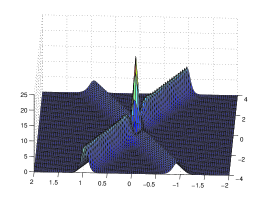
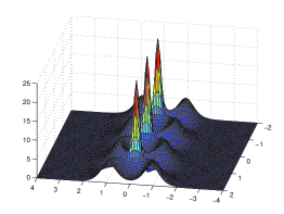
Figure 1 shows two particular types of the dynamics of $2$-solitons: scattering of two solitons with nonequal speeds for $\xi_{1}\neq\xi_{2}$ (left) and oscillations of bound states of two solitons with equal speeds for $\xi_{1}=\xi_{2}$ (right) if $\eta_{1}\neq\eta_{2}$. Note that the solution becomes zero if $\xi_{1}=\xi_{2}$ and $\eta_{1}=\eta_{2}$.

Refer to caption
Refer to caption
Figure 1. Surface plots of $|q^{S}|^{2}$ versus $(x,t)$ for the $2$-soliton solutions (4.4) with $\eta_{1}=1$, $\eta_{2}=1.5$, and either $\xi_{1}=-\xi_{2}=1$ (left) or $\xi_{1}=\xi_{2}=0$ (right). Other translation parameters are set to zero.

5. Analysis of neighborhood of multi-solitons

We shall now consider the dressing transformation for small but nonzero $q_{0}$ in $L^{2}(\mathbb{R})$. Recall that the $L^{2}(\mathbb{R})$ norm of a solution of the cubic NLS equation (1.1) is conserved in time $t$. To work with the dressing transformation, we consider a classical solution $q_{0}$ of the cubic NLS equation (1.1) in $L^{2}(\mathbb{R})$ with constant $\|q_{0}\|_{L^{2}(\mathbb{R})}$.

Let $s_{j}$ be solutions of the spectral problems (2.4) and (3.4) associated with small but nonzero $q_{0}$ in $L^{2}(\mathbb{R})$ for $z_{j}=\xi_{j}+i\eta_{j}$ with $\eta_{j}>0$. We write this vector in the separable form

(5.1) $$s_{j}:=e^{-i\bar{z}_{j}(x-x_{j})-2i\bar{z}_{j}^{2}t+i\theta_{j}}f_{j}-e^{i\bar{z}_{j}(x-x_{j})+2i\bar{z}_{j}^{2}t-i\theta_{j}}g_{j}$$

where $(x_{j},\theta_{j})$ are arbitrary real parameters and components of the $2$-vectors $f_{j}=(\mathfrak{a}_{1}^{j},\mathfrak{a}_{2}^{j})$ and $g_{j}=(\mathfrak{b}_{1}^{j},\mathfrak{b}_{2}^{j})$ satisfy the boundary conditions

(5.2) $$\left\{\begin{array}[]{l}\lim\limits_{x\to-\infty}\mathfrak{a}_{1}^{j}=1,\\ \lim\limits_{x\to+\infty}e^{-2i\bar{z}_{j}(x-x_{j})-4i\bar{z}_{j}^{2}t+2i\theta_{j}}\mathfrak{a}_{2}^{j}=0,\end{array}\right.$$

and

(5.3) $$\left\{\begin{array}[]{l}\lim\limits_{x\to-\infty}e^{2i\bar{z}_{j}(x-x_{j})+4i\bar{z}_{j}^{2}t-2i\theta_{j}}\mathfrak{b}_{1}^{j}=0,\\ \lim\limits_{x\to+\infty}\mathfrak{b}_{2}^{j}=1.\end{array}\right.$$

If $q_{0}=0$, then we have unique solutions $f_{j}=(1,0)$ and $g_{j}=(0,1)$, so that the separable form (5.1) recovers (4.1). Using the same analysis as in Lemmas 4.1 and 4.3 of [15], we obtain the following result.

Proposition 5.1.

Let $q_{0}$ be a classical solution of the cubic NLS equation (1.1) in $L^{2}(\mathbb{R})$. There exists a positive constant $\epsilon_{0}$ such that if $\|q_{0}\|_{L^{2}}\leq\epsilon_{0}$, then the spectral problems (2.4) and (3.4) for $z_{j}=\xi_{j}+i\eta_{j}$ admit a solution $s_{j}$ satisfying (5.1), (5.2) and (5.3). For all $t\in\mathbb{R}$, components of $f_{j}=(\mathfrak{a}_{1}^{j},\mathfrak{a}_{2}^{j})$ and $g_{j}=(\mathfrak{b}_{1}^{j},\mathfrak{b}_{2}^{j})$ belong to the class

(5.4) $$(\mathfrak{a}_{1}^{j},\mathfrak{a}_{2}^{j})\in L^{\infty}(\mathbb{R})\times(L^{\infty}(\mathbb{R})\cap L^{2}(\mathbb{R})),\quad(\mathfrak{b}_{1}^{j},\mathfrak{b}_{2}^{j})\in(L^{\infty}(\mathbb{R})\cap L^{2}(\mathbb{R}))\times L^{\infty}(\mathbb{R}),$$

and there exists a positive $q_{0}$-independent constant $C$ such that

(5.5) $\displaystyle\left\|\mathfrak{a}_{1}^{j}-1\right\|_{L^{\infty}}+\left\|\mathfrak{a}_{2}^{j}\right\|_{L^{2}\cap L^{\infty}}+\left\|\mathfrak{b}_{1}^{j}\right\|_{L^{2}\cap L^{\infty}}+\left\|\mathfrak{b}_{2}^{j}-1\right\|_{L^{\infty}}\leq C\left\|q_{0}\right\|_{L^{2}}.$

We now construct a neighborhood of a multi-soliton by using the dressing transformation in Propositions 2.2 and 3.1. The arguments are valid for all multi-solitons, but we give details of analysis in the case of $2$-solitons, because of the nature of the perturbations yielding page-long computations. At the end of the section, we summarize the key steps and modifications required to obtain the result in the general case $n\geq 1$.

Let $M$, $\Sigma$, and $F$ be the matrices defined by (2.5), (4.2), and (4.3), associated to $s_{1}$ and $s_{2}$ as given in (5.1). Let $M^{S}$, $\Sigma^{S}$, and $F^{S}$ be the matrices corresponding to the 2-soliton $q^{S}$ given by (4.4). We denote $D=\det(M)$ and $D^{S}=\det(M^{S})$. The following result tells us that if $q_{0}\in L^{2}$ is small, then the transformation formula (3.2) with $s_{1}$ and $s_{2}$ given by (5.1) yields a new solution $q$ near the $2$-soliton $q^{S}$ in the $L^{2}$ norm.

Proposition 5.2.

Let $q_{0}$ be a classical solution of the cubic NLS equation (1.1) in $L^{2}(\mathbb{R})$ and $q^{S}$ be the $2$-soliton given explicitly by (4.4) with $(\xi_{1},\eta_{1})\neq(\xi_{2},\eta_{2})$. There exists a positive constant $\epsilon_{0}$ such that if $\|q_{0}\|_{L^{2}}\leq\epsilon_{0}$, then there exists a positive $q_{0}$-independent constant $C$ such that the function $q$ given by the transformation formula (3.2) with the functions $s_{1}$ and $s_{2}$ in (5.1), (5.2) and (5.3) satisfies

(5.6) $$\left\|q-q^{S}\right\|_{L^{2}}\leq C\|q_{0}\|_{L^{2}},\quad t\in\mathbb{R}.$$
Proof.

For convenience, we express bound (5.6) as $\left\|q-q^{S}\right\|_{L^{2}}\lesssim\epsilon$ with $\epsilon:=\left\|q_{0}\right\|_{L^{2}}$ and use these notations in the rest of the paper. The bound (5.6) follows from the triangle inequality if we can show that

(5.7) $$\left\|\frac{2\Sigma}{D}-q^{S}\right\|_{L^{2}}\lesssim\epsilon.$$

In turn, since in this case $D_{i,j}=(-1)^{i+j}M_{3-i,3-j},$ this bound will be a consequence of the bounds

(5.8) $$\left\|\frac{F_{1,1}M_{2,2}}{D}-\frac{F^{S}_{1,1}M^{S}_{2,2}}{D^{S}}\right\|_{L^{2}},\quad\left\|\frac{F_{2,2}M_{1,1}}{D}-\frac{F^{S}_{2,2}M^{S}_{1,1}}{D^{S}}\right\|_{L^{2}}\lesssim\epsilon$$

and

(5.9) $$\left\|\frac{F_{2,1}M_{1,2}}{D}-\frac{F^{S}_{2,1}M^{S}_{1,2}}{D^{S}}\right\|_{L^{2}},\quad\left\|\frac{F_{1,2}M_{2,1}}{D}-\frac{F^{S}_{1,2}M^{S}_{2,1}}{D^{S}}\right\|_{L^{2}}\lesssim\epsilon.$$

In fact, to prove (5.8) and (5.9), it will suffice to show the estimates for $F_{1,1}M_{2,2}$ and $F_{2,1}M_{1,2}$, since the estimates for $F_{2,2}M_{1,1}$ and $F_{1,2}M_{2,1}$ are analogous.

We divide the proof into three steps. In the first step, we write down global estimates in $L^{2}(\mathbb{R})$ and $L^{\infty}(\mathbb{R})$ measuring the discrepancy between $(F,M)$ and $(F^{S},M^{S}).$ From these, in the second step, we obtain for any $t\in\mathbb{R}$ that

$$\left\|\frac{2\Sigma}{D}-\frac{2\Sigma^{S}}{D^{S}}\right\|_{L^{\infty}([-R,R])}\lesssim\epsilon,$$

for some $R$ large but fixed.

Finally, the growth properties of $D$ (and $D^{S}$) together with the $L^{2}(\mathbb{R})$ control on the difference between $(F,M)$ and $(F^{S},M^{S})$ obtained in the first part, allows us to derive the result outside a compact set. This result together with the $L^{\infty}([-R,R])$ estimate from the second step yields the desired conclusion.

Step 1: Global estimates for $M_{1,2},M_{2,2},F_{2,1}$ and $F_{1,1}$
From (5.1), we have

$\displaystyle M_{1,2}=\frac{1}{\eta_{1}+\eta_{2}+i(\xi_{1}-\xi_{2})}\Big{[}e^{-\eta_{2}\varphi_{2}-i\psi_{2}-\eta_{1}\varphi_{1}+i\psi_{1}}(\mathfrak{a}_{1}^{2}\mathfrak{a}_{1}^{1}+\mathfrak{a}_{2}^{2}\mathfrak{a}_{2}^{1})-e^{\eta_{2}\varphi_{2}+i\psi_{2}-\eta_{1}\varphi_{1}+i\psi_{1}}$
$\displaystyle\times(\mathfrak{b}_{1}^{2}\mathfrak{a}_{1}^{1}+\mathfrak{b}_{2}^{2}\mathfrak{a}_{2}^{1})-e^{-\eta_{2}\varphi_{2}-i\psi_{2}+\eta_{1}\varphi_{1}-i\psi_{1}}(\mathfrak{a}_{1}^{2}\mathfrak{b}_{1}^{1}+\mathfrak{a}_{2}^{2}\mathfrak{b}_{2}^{1})+e^{\eta_{2}\varphi_{2}+i\psi_{2}+\eta_{1}\varphi_{1}-i\psi_{1}}(\mathfrak{b}_{1}^{2}\mathfrak{b}_{1}^{1}+\mathfrak{b}_{2}^{2}\mathfrak{b}_{2}^{1})\Big{]}.$

Using inequality (5.5), we expand this expression as follows:

$\displaystyle M_{1,2}$ $\displaystyle=$ $\displaystyle\frac{1}{\eta_{1}+\eta_{2}+i(\xi_{1}-\xi_{2})}\Big{[}e^{-\eta_{2}\varphi_{2}-i\psi_{2}-\eta_{1}\varphi_{1}+i\psi_{1}}$
$\displaystyle\times[(1+\mathcal{O}_{L^{\infty}}(\epsilon))(1+\mathcal{O}_{L^{\infty}}(\epsilon))+\mathcal{O}_{L^{2}\cap L^{\infty}}(\epsilon)\mathcal{O}_{L^{2}\cap L^{\infty}}(\epsilon)]$
$\displaystyle-e^{\eta_{2}\varphi_{2}+i\psi_{2}-\eta_{1}\varphi_{1}+i\psi_{1}}[\mathcal{O}_{L^{2}\cap L^{\infty}}(\epsilon)(1+\mathcal{O}_{L^{\infty}}(\epsilon))+(1+\mathcal{O}_{L^{\infty}}(\epsilon))\mathcal{O}_{L^{2}\cap L^{\infty}}(\epsilon)]$
$\displaystyle-e^{-\eta_{2}\varphi_{2}-i\psi_{2}+\eta_{1}\varphi_{1}-i\psi_{1}}[(1+\mathcal{O}_{L^{\infty}}(\epsilon))\mathcal{O}_{L^{2}\cap L^{\infty}}(\epsilon)+\mathcal{O}_{L^{2}\cap L^{\infty}}(\epsilon)(1+\mathcal{O}_{L^{\infty}}(\epsilon))]$
$\displaystyle+e^{\eta_{2}\varphi_{2}+i\psi_{2}+\eta_{1}\varphi_{1}-i\psi_{1}}[\mathcal{O}_{L^{2}\cap L^{\infty}}(\epsilon)\mathcal{O}_{L^{2}\cap L^{\infty}}(\epsilon)+(1+\mathcal{O}_{L^{\infty}}(\epsilon))(1+\mathcal{O}_{L^{\infty}}(\epsilon))]\Big{]}$
$\displaystyle=$ $\displaystyle\frac{(e^{-\eta_{2}\varphi_{2}-i\psi_{2}-\eta_{1}\varphi_{1}+i\psi_{1}}+e^{\eta_{2}\varphi_{2}+i\psi_{2}+\eta_{1}\varphi_{1}-i\psi_{1}})}{\eta_{1}+\eta_{2}+i(\xi_{1}-\xi_{2})}$
$\displaystyle+\frac{(e^{-\eta_{2}\varphi_{2}-i\psi_{2}-\eta_{1}\varphi_{1}+i\psi_{1}}+e^{\eta_{2}\varphi_{2}+i\psi_{2}+\eta_{1}\varphi_{1}-i\psi_{1}})}{\eta_{1}+\eta_{2}+i(\xi_{1}-\xi_{2})}[\mathcal{O}_{L^{\infty}}(\epsilon)+\mathcal{O}_{L^{2}\cap L^{\infty}}(\epsilon)]$
$\displaystyle-\frac{(e^{\eta_{2}\varphi_{2}+i\psi_{2}-\eta_{1}\varphi_{1}+i\psi_{1}}+e^{-\eta_{2}\varphi_{2}-i\psi_{2}+\eta_{1}\varphi_{1}-i\psi_{1}})}{\eta_{1}+\eta_{2}+i(\xi_{1}-\xi_{2})}\mathcal{O}_{L^{2}\cap L^{\infty}}(\epsilon),$

which yields

$\displaystyle M_{1,2}$ $\displaystyle=$ $\displaystyle M_{1,2}^{S}+M_{1,2}^{S}[\mathcal{O}_{L^{\infty}}(\epsilon)+\mathcal{O}_{L^{2}\cap L^{\infty}}(\epsilon)]$
$\displaystyle-\frac{(e^{\eta_{2}\varphi_{2}+i\psi_{2}-\eta_{1}\varphi_{1}+i\psi_{1}}+e^{-\eta_{2}\varphi_{2}-i\psi_{2}+\eta_{1}\varphi_{1}-i\psi_{1}})}{\eta_{1}+\eta_{2}+i(\xi_{1}-\xi_{2})}\mathcal{O}_{L^{2}\cap L^{\infty}}(\epsilon),$

where $\mathcal{O}_{L^{\infty}}(\epsilon)$ means that the function is $\mathcal{O}(\epsilon)$ small in the $L^{\infty}(\mathbb{R})$ norm. In the same way, we are able to show that

(5.11) $$M_{2,2}=M_{2,2}^{S}+M_{2,2}^{S}[\mathcal{O}_{L^{\infty}}(\epsilon)+\mathcal{O}_{L^{2}\cap L^{\infty}}(\epsilon)]-\frac{(e^{-2i\psi_{2}}+e^{2i\psi_{2}})}{2\eta_{2}}\mathcal{O}_{L^{2}\cap L^{\infty}}(\epsilon).$$

One can see that similar asymptotics hold for $M_{2,1}$ and $M_{1,1}$ which in turn yield the following expansion of $D$:

(5.12) $$D=D^{S}+D^{S}\mathcal{O}_{L^{\infty}}(\epsilon)+(E_{1}+E_{2})\mathcal{O}_{L^{2}\cap L^{\infty}}(\epsilon).$$

where

(5.13) $\displaystyle E_{1}$ $\displaystyle=$ $\displaystyle\left[\frac{1}{4\eta_{1}\eta_{2}}+\frac{1}{(\eta_{1}+\eta_{2})^{2}+(\xi_{1}-\xi_{2})^{2}}\right]\left[e^{2\eta_{2}\varphi_{2}-2\eta_{1}\varphi_{1}}+e^{-2\eta_{2}\varphi_{2}+2\eta_{1}\varphi_{1}}+e^{2i\psi_{2}+2i\psi_{1}}\right.$
$\displaystyle\left.+e^{-2i\psi_{2}-2i\psi_{1}}+e^{2\eta_{2}\varphi_{2}+2i\psi_{1}}+e^{-2\eta_{2}\varphi_{2}-2i\psi_{1}}+e^{2\eta_{1}\varphi_{1}-2i\psi_{2}}+e^{-2\eta_{1}\varphi_{1}+2i\psi_{2}}\right]$

and

(5.14) $\displaystyle E_{2}$ $\displaystyle=$ $\displaystyle\left[\frac{1}{4\eta_{1}\eta_{2}}-\frac{1}{(\eta_{1}+\eta_{2})^{2}+(\xi_{1}-\xi_{2})^{2}}\right]\left[e^{2\eta_{2}\varphi_{2}+2\eta_{1}\varphi_{1}}+e^{-2\eta_{2}\varphi_{2}-2\eta_{1}\varphi_{1}}+e^{2i\psi_{2}-2i\psi_{1}}\right.$
$\displaystyle\left.+e^{-2i\psi_{2}+2i\psi_{1}}+e^{2\eta_{2}\varphi_{2}-2i\psi_{1}}+e^{-2\eta_{2}\varphi_{2}+2i\psi_{1}}+e^{2\eta_{1}\varphi_{1}+2i\psi_{2}}+e^{-2\eta_{1}\varphi_{1}-2i\psi_{2}}\right].$

We claim $D=D^{S}(1+\mathcal{O}_{L^{\infty}}(\epsilon)),$ which has as a consequence

(5.15) $$\frac{1}{D}=\frac{1}{D^{S}(1+\mathcal{O}_{L^{\infty}}(\epsilon))}=\frac{1+\mathcal{O}_{L^{\infty}}(\epsilon)}{D^{S}}.$$

Indeed, assuming $(\eta_{1},\xi_{1})\neq(\eta_{2},\xi_{2})$ and letting $\gamma=2\eta_{1}\eta_{2}\left((\eta_{1}+\eta_{2})^{2}+(\xi_{1}-\xi_{2})^{2}\right)$, it is clear that

(5.16) $\displaystyle\gamma^{-1}\left|D^{S}\right|$ $\displaystyle=$ $\displaystyle\left((\eta_{1}+\eta_{2})^{2}+(\xi_{1}-\xi_{2})^{2}\right)\Big{(}\cosh\big{(}2(\eta_{1}\varphi_{1}+\eta_{2}\varphi_{2})\big{)}+\cosh\big{(}2(\eta_{1}\varphi_{1}-\eta_{2}\varphi_{2})\big{)}\Big{)}$
$\displaystyle-4\eta_{1}\eta_{2}\Big{(}\cosh\big{(}2(\eta_{1}\varphi_{1}+\eta_{2}\varphi_{2})\big{)}+\cos\big{(}2(\psi_{1}-\psi_{2})\big{)}\Big{)}$
$\displaystyle=$ $\displaystyle\left((\eta_{1}-\eta_{2})^{2}+(\xi_{1}-\xi_{2})^{2}\right)\cosh\big{(}2(\eta_{1}\varphi_{1}+\eta_{2}\varphi_{2})\big{)}$
$\displaystyle+\left((\eta_{1}+\eta_{2})^{2}+(\xi_{1}-\xi_{2})^{2}\right)\cosh\big{(}2(\eta_{1}\varphi_{1}-\eta_{2}\varphi_{2})\big{)}-4\eta_{1}\eta_{2}\cos\big{(}2(\psi_{1}-\psi_{2})\big{)}$
$\displaystyle\gtrsim$ $\displaystyle\cosh\big{(}2(\eta_{1}\varphi_{1}+\eta_{2}\varphi_{2})\big{)}+\cosh\big{(}2(\eta_{1}\varphi_{1}-\eta_{2}\varphi_{2})\big{)},$

because $(\eta_{1}+\eta_{2})^{2}+(\xi_{1}-\xi_{2})^{2}>4\eta_{1}\eta_{2}$ and $\cosh 2(\eta_{1}\varphi_{1}-\eta_{2}\varphi_{2})\geq 1\geq\cos(\psi_{1}-\psi_{2}).$ Using this estimate, we obtain

$$\left|E_{1}\right|\lesssim\cosh\big{(}2(\eta_{2}\varphi_{2}-\eta_{1}\varphi_{1})\big{)}\lesssim\left|D^{S}\right|.$$

Since

$$\cosh(2\eta_{1}\varphi_{1})+\cosh(2\eta_{2}\varphi_{2})\lesssim\cosh\big{(}2(\eta_{1}\varphi_{1}+\eta_{2}\varphi_{2})\big{)}+\cosh\big{(}2(\eta_{1}\varphi_{1}-\eta_{2}\varphi_{2})\big{)},$$

we also have

$$\left|E_{2}\right|\lesssim\cosh\big{(}2(\eta_{1}\varphi_{1}+\eta_{2}\varphi_{2})\big{)}+\cosh(2\eta_{1}\varphi_{1})+\cosh(2\eta_{2}\varphi_{2})\lesssim\left|D^{S}\right|,$$

from which the claim follows.

We turn to the asymptotics for $F.$ $F_{2,1}$ satisfies the following

(5.17) $\displaystyle F_{2,1}=F_{2,1}^{S}+F_{2,1}^{S}\mathcal{O}_{L^{\infty}}(\epsilon)$
$\displaystyle\phantom{texttest}+[e^{\eta_{2}\varphi_{2}-i\psi_{2}+\eta_{1}\varphi_{1}+i\psi_{1}}+e^{-\eta_{2}\varphi_{2}+i\psi_{2}-\eta_{1}\varphi_{1}-i\psi_{1}}-e^{\eta_{2}\varphi_{2}-i\psi_{2}-\eta_{1}\varphi_{1}-i\psi_{1}}]\mathcal{O}_{L^{2}\cap L^{\infty}}(\epsilon),$

while $F_{1,1}$ can be expanded as

(5.18) $\displaystyle F_{1,1}=F_{1,1}^{S}+F_{1,1}^{S}\mathcal{O}_{L^{\infty}}(\epsilon)+[e^{2\eta_{1}\varphi_{1}}+e^{-2\eta_{1}\varphi_{1}}-e^{-2i\psi_{1}}]\mathcal{O}_{L^{2}\cap L^{\infty}}(\epsilon).$

Step 2: Estimates on a compact set.

Let $R>0$ be a large constant independent of $\epsilon$ (and $t$) to be fixed later. The purpose of this point is to obtain asymptotics of $F_{1,1}M_{2,2}$ and $F_{2,1}M_{1,2}$ on the compact set $\{\left|x\right|<R\}$ (for all $t\in\mathbb{R}$). For our goal, it is enough to show that these terms differ from $F^{S}_{1,1}M^{S}_{2,2}$ and $F^{S}_{2,1}M^{S}_{1,2}$ respectively, by a quantity uniformly controlled by $\epsilon.$

To this end, we note that on the compact set, the previous estimates (5)–(5.18) yield

(5.19) $$\left|F_{1,1}M_{2,2}-F^{S}_{1,1}M^{S}_{2,2}\right|\lesssim\cosh\big{(}2(\eta_{1}\varphi_{1}+\eta_{2}\varphi_{2})\big{)}+\cosh\big{(}2(\eta_{1}\varphi_{1}-\eta_{2}\varphi_{2})\big{)}$$

and

(5.20) $$\left|F_{2,1}M_{1,2}-F^{S}_{2,1}M^{S}_{1,2}\right|\lesssim\cosh\big{(}2(\eta_{1}\varphi_{1}+\eta_{2}\varphi_{2})\big{)}+\cosh\big{(}2(\eta_{1}\varphi_{1}-\eta_{2}\varphi_{2})\big{)},$$

where $\mathcal{O}_{L^{\infty}}(\epsilon)$ is now used in the $L^{\infty}([-R,R])$ norm.

From (5.15) and (5.16), we observe that

(5.21) $$\left|D\right|\gtrsim\left|D^{S}\right|\gtrsim\cosh\big{(}2(\eta_{1}\varphi_{1}+\eta_{2}\varphi_{2})\big{)}+\cosh\big{(}2(\eta_{1}\varphi_{1}-\eta_{2}\varphi_{2})\big{)},$$

so that

(5.22) $\displaystyle\left|\frac{F_{1,1}M_{2,2}}{D}-\frac{F^{S}_{1,1}M^{S}_{2,2}}{D^{S}}\right|$ $\displaystyle=$ $\displaystyle\left|\frac{F_{1,1}M_{2,2}}{D^{S}}(1+\mathcal{O}_{L^{\infty}}(\epsilon))-\frac{F^{S}_{1,1}M^{S}_{2,2}}{D^{S}}\right|$
$\displaystyle\lesssim$ $\displaystyle\left|\frac{F_{1,1}M_{2,2}}{D^{S}}-\frac{F^{S}_{1,1}M^{S}_{2,2}}{D^{S}}\right|+\mathcal{O}_{L^{\infty}}(\epsilon)\left|\frac{F_{1,1}M_{2,2}}{D^{S}}\right|$
$\displaystyle=$ $\displaystyle\mathcal{O}_{L^{\infty}}(\epsilon).$

Similarly, one has

(5.23) $$\left|\frac{F_{2,1}M_{1,2}}{D}-\frac{F^{S}_{2,1}M^{S}_{1,2}}{D^{S}}\right|=\mathcal{O}_{L^{\infty}}(\epsilon),$$

thanks to (5.19) and (5.20).


Step 3: Estimates outside a compact set.

We now deal with the estimates outside the compact set $\{\left|x\right|<R\}$ for the same $R$ as in Step 2. Here, the norms $L^{2},$ $L^{\infty}$ are taken outside the compact set $\{\left|x\right|<R\}$. Again, from (5)–(5.18), we have

$\displaystyle F_{11}M_{22}=F_{11}^{S}M_{22}^{S}$ $\displaystyle-$ $\displaystyle\frac{1}{2\eta_{2}}\left(e^{-2\eta_{2}\varphi_{2}+2i\psi_{1}}+e^{2\eta_{2}\varphi_{2}+2i\psi_{1}}\right)\mathcal{O}_{L^{\infty}}(\epsilon)$
$\displaystyle-$ $\displaystyle\frac{1}{2\eta_{2}}(e^{-2\eta_{1}\varphi_{1}}+e^{2\eta_{1}\varphi_{1}})(e^{2i\psi_{2}}+e^{-2i\psi_{2}})\mathcal{O}_{L^{\infty}}(\epsilon)$
$\displaystyle+$ $\displaystyle\frac{1}{2\eta_{2}}(e^{-2\eta_{2}\varphi_{2}}+e^{2\eta_{2}\varphi_{2}})(e^{-2\eta_{1}\varphi_{1}}+e^{2\eta_{1}\varphi_{1}})\mathcal{O}_{L^{2}\cap L^{\infty}}(\epsilon),$

and

(5.25) $\displaystyle F_{2,1}M_{1,2}=F^{S}_{2,1}M^{S}_{1,2}+\frac{1}{\eta_{1}+\eta_{2}+i(\xi_{1}-\xi_{2})}\left[G_{1}\mathcal{O}_{L^{\infty}}(\epsilon)+G_{2}\mathcal{O}_{L^{2}\cap L^{\infty}}(\epsilon)\right],$

where

$\displaystyle G_{1}$ $\displaystyle=$ $\displaystyle-e^{-\eta_{2}\varphi_{2}+i\psi_{2}+\eta_{1}\varphi_{1}+i\psi_{1}}(e^{-\eta_{2}\varphi_{2}-i\psi_{2}-\eta_{1}\varphi_{1}+i\psi_{1}}+e^{\eta_{2}\varphi_{2}+i\psi_{2}+\eta_{1}\varphi_{1}-i\psi_{1}}),$
$\displaystyle G_{2}$ $\displaystyle=$ $\displaystyle e^{-\eta_{2}\varphi_{2}+i\psi_{2}+\eta_{1}\varphi_{1}+i\psi_{1}}(e^{\eta_{2}\varphi_{2}+i\psi_{2}-\eta_{1}\varphi_{1}+i\psi_{1}}+e^{-\eta_{2}\varphi_{2}-i\psi_{2}+\eta_{1}\varphi_{1}-i\psi_{1}})$
$\displaystyle+(e^{\eta_{2}\varphi_{2}-i\psi_{2}+\eta_{1}\varphi_{1}+i\psi_{1}}+e^{-\eta_{2}\varphi_{2}+i\psi_{2}-\eta_{1}\varphi_{1}-i\psi_{1}})(e^{-\eta_{2}\varphi_{2}-i\psi_{2}-\eta_{1}\varphi_{1}+i\psi_{1}}+e^{\eta_{2}\varphi_{2}+i\psi_{2}+\eta_{1}\varphi_{1}-i\psi_{1}})$
$\displaystyle-e^{\eta_{2}\varphi_{2}-i\psi_{2}-\eta_{1}\varphi_{1}-i\psi_{1}}(e^{-\eta_{2}\varphi_{2}-i\psi_{2}-\eta_{1}\varphi_{1}+i\psi_{1}}+e^{\eta_{2}\varphi_{2}+i\psi_{2}+\eta_{1}\varphi_{1}-i\psi_{1}})$
$\displaystyle+(e^{\eta_{2}\varphi_{2}-i\psi_{2}+\eta_{1}\varphi_{1}+i\psi_{1}}+e^{-\eta_{2}\varphi_{2}+i\psi_{2}-\eta_{1}\varphi_{1}-i\psi_{1}})(-e^{\eta_{2}\varphi_{2}+i\psi_{2}-\eta_{1}\varphi_{1}+i\psi_{1}}-e^{-\eta_{2}\varphi_{2}-i\psi_{2}+\eta_{1}\varphi_{1}-i\psi_{1}})$
$\displaystyle-e^{\eta_{2}\varphi_{2}-i\psi_{2}-\eta_{1}\varphi_{1}-i\psi_{1}}(-e^{\eta_{2}\varphi_{2}+i\psi_{2}-\eta_{1}\varphi_{1}+i\psi_{1}}-e^{-\eta_{2}\varphi_{2}-i\psi_{2}+\eta_{1}\varphi_{1}-i\psi_{1}}).$

From these estimates, we obtain

$\displaystyle\left|F_{1,1}M_{2,2}-F^{S}_{11}M^{S}_{2,2}\right|$ $\displaystyle\lesssim$ $\displaystyle\mathcal{O}_{L^{2}\cap L^{\infty}}(\epsilon)+(H_{1}+H_{2})\mathcal{O}_{L^{\infty}}(\epsilon)+H_{1}H_{2}\;\mathcal{O}_{L^{2}\cap L^{\infty}}(\epsilon),$

where

$\displaystyle H_{1}$ $\displaystyle=$ $\displaystyle-(e^{-2\eta_{1}\varphi_{1}}+e^{2\eta_{1}\varphi_{1}})(e^{2i\psi_{2}}+e^{-2i\psi_{2}}),$
$\displaystyle H_{2}$ $\displaystyle=$ $\displaystyle-(e^{-2\eta_{2}\varphi_{2}+2i\psi_{1}}+e^{2\eta_{2}\varphi_{2}+2i\psi_{1}}).$

We can see these functions satisfy the bounds

(5.26) $$\left|H_{i}\right|\lesssim\cosh(2\eta_{i}\varphi_{i}),\quad\mbox{ for }i=1,2.$$

In the same way, we have

$\displaystyle\left|F_{2,1}M_{1,2}-F^{S}_{2,1}M^{S}_{1,2}\right|$ $\displaystyle\lesssim$ $\displaystyle J_{1}J_{3}\mathcal{O}_{L^{\infty}}(\epsilon)$
$\displaystyle+(J_{1}J_{4}+J_{3}^{2}+J_{2}J_{3}+J_{3}J_{4}+J_{2}J_{4})\mathcal{O}_{L^{2}\cap L^{\infty}}(\epsilon),$

where

$\displaystyle J_{1}$ $\displaystyle=$ $\displaystyle-e^{-\eta_{2}\varphi_{2}+\eta_{1}\varphi_{1}},$
$\displaystyle J_{2}$ $\displaystyle=$ $\displaystyle-e^{\eta_{2}\varphi_{2}-\eta_{1}\varphi_{1}},$
$\displaystyle J_{3}$ $\displaystyle=$ $\displaystyle e^{-\eta_{2}\varphi_{2}-\eta_{1}\varphi_{1}}+e^{\eta_{2}\varphi_{2}+\eta_{1}\varphi_{1}},$
$\displaystyle J_{4}$ $\displaystyle=$ $\displaystyle-e^{\eta_{2}\varphi_{2}-\eta_{1}\varphi_{1}}-e^{-\eta_{2}\varphi_{2}+\eta_{1}\varphi_{1}}.$

It is immediate from (5.26) that

(5.28) $$\left|H_{1}H_{2}\right|\lesssim\cosh(2(\eta_{1}\varphi_{1}+\eta_{2}\varphi_{2}))+\cosh(2(\eta_{1}\varphi_{1}-\eta_{2}\varphi_{2})).$$

In a similar fashion, we deduce from (5) that

$\displaystyle\left|J_{1}J_{4}\right|\lesssim e^{-2\eta_{2}\varphi_{2}}+e^{2\eta_{1}\varphi_{1}},$
$\displaystyle\left|J_{2}J_{4}\right|\lesssim 1+e^{2\eta_{2}\varphi_{2}-2\eta_{1}\varphi_{1}},$
$\displaystyle\left|J_{3}^{2}\right|\lesssim\cosh(2\eta_{2}\varphi_{2}+2\eta_{1}\varphi_{1})+1,$
$\displaystyle\left|J_{3}J_{4}\right|\lesssim\cosh(2\eta_{1}\varphi_{1})+\cosh(2\eta_{2}\varphi_{2}).$

All these quantities can be bounded from above by $\left|D\right|,$ in light of (5.15) and (5.16). Thus, we can assert that $\frac{H_{1}H_{2}}{D},\frac{J_{1}J_{4}}{D},$ $\frac{J_{3}^{2}}{D},\frac{J_{2}J_{4}}{D}$ and $\frac{J_{3}J_{4}}{D}$ are $L^{\infty}$ functions whose norms are bounded uniformly in $t.$

Now we show that $\frac{H_{1}}{D},\frac{H_{2}}{D},\frac{J_{1}J_{3}}{D}$ and $\frac{J_{2}J_{3}}{D}$ are bounded in $L^{2},$ uniformly in $t.$ From (5.28) and similar estimates, we see that it suffices to prove that $\frac{e^{2\eta_{1}\varphi_{1}}}{D}\in L^{2}$ (the terms $\frac{e^{-2\eta_{1}\varphi_{1}}}{D},$ $e^{\pm 2\eta_{2}\varphi_{2}}$ can be dealt with similarly).

Appealing once again to (5.15) and (5.16) we see that

(5.29) $\displaystyle\frac{e^{-2\eta_{1}\varphi_{1}}}{\left|D\right|}$ $\displaystyle\lesssim$ $\displaystyle\frac{e^{-2\eta_{1}\varphi_{1}}}{\cosh(2(\eta_{1}\varphi_{1}+\eta_{2}\varphi_{2}))+\cosh(2(\eta_{1}\varphi_{1}-\eta_{2}\varphi_{2}))}$
$\displaystyle\lesssim$ $\displaystyle\frac{e^{-2\eta_{1}\varphi_{1}}}{e^{2\eta_{2}\varphi_{2}+2\eta_{1}\varphi_{1}}+e^{-2\eta_{2}\varphi_{2}+2\eta_{1}\varphi_{1}}}\lesssim\mbox{sech}(2\eta_{2}\varphi_{2})\in L^{2}.$

Collecting all these estimates, we see that outside the compact set $\{\left|x\right|<R\}$

(5.30) $$\frac{F_{1,1}M_{2,2}}{D}=\frac{F_{1,1}^{S}M_{2,2}^{S}}{D^{S}}+\mathcal{O}_{L^{2}}(\epsilon)$$

and

(5.31) $$\frac{F_{1,2}M_{1,2}}{D}=\frac{F_{1,2}^{S}M_{1,2}^{S}}{D^{S}}+\mathcal{O}_{L^{2}}(\epsilon).$$

Combining (5.22), (5.23), (5.30) and (5.31), we obtain (5.6). ∎

Corollary 5.3.

Under conditions of Proposition 5.2, there is a positive constant $C$ such that

(5.32) $$\|q_{0}\|_{L^{2}}\leq C\left\|q-q^{S}\right\|_{L^{2}},\quad t\in\mathbb{R}.$$
Proof.

Because the dressing transformation formulas (2.3) and (3.2) are invertible by the construction, the bound (5.32) follows from the triangle inequality and bound (5.7). ∎

Remark 5.4.

Proposition 5.2 can be extended to the general case of multi-soliton configurations. The global estimates obtained in (5)–(5.18) can be used to derive explicit (though cumbersome) expansions for the $D_{j,k}$’s (including the determinant $D$). On the compact set $\{\left|x\right|<R\}$, the $\mathcal{O}_{L^{\infty}}(\varepsilon)$ difference between $D_{j,k}F_{j,k}$’s and $D_{j,k}^{S}F_{j,k}^{S}$’s together with

$$\frac{1}{D}=\frac{1}{D^{S}}(1+\mathcal{O}_{L^{\infty}(\varepsilon)})$$

suffices to show

$$\frac{\Sigma}{D}=\frac{\Sigma^{S}}{D^{S}}+\mathcal{O}_{L^{\infty}}(\varepsilon)$$

for all $t\in\mathbb{R}$. The estimates outside the compact set $\{\left|x\right|<R\}$ can be achieved as in the third step, thanks to the bound

(5.33) $$e^{2\left(\sum_{i=1}^{n}\sigma_{i}\eta_{i}\varphi_{i}\right)}\lesssim\left|D\right|,$$

valid for any choice of signs $\sigma:\{1,\ldots,n\}\to\{-1,1\},$ and making use of the fact that for any $j\in\{1,\ldots,n\},$

(5.34) $$\frac{e^{2\sum_{i\neq j}\sigma_{i}\eta_{i}\varphi_{i}}}{\left|D\right|}\lesssim\mbox{sech }2\eta_{j}\varphi_{j},$$

which is in $L^{2}$ with norm bounded independent of $t.$ The estimates thus obtained can be seen to be independent of the time, thanks to the conservation of the $L^{2}(\mathbb{R})$ norm of the solution $q_{0}$ of the cubic NLS equation (1.1).

6. Orbital stability of multi-solitons

In this section we prove the result on the orbital stability of multi-solitons in $L^{2}(\mathbb{R})$ given by Theorem 1.6. First, we will assume that the initial data $q_{0}$ for the cubic NLS equation (1.1) satisfies the bound (1.4) (that is, it is close the multi-soliton $q^{S}$) and belongs to $H^{3}(\mathbb{R})$. By the well-posedness theory for the NLS equation [8, 13], there exists a unique solution in class

$$q\in C^{0}(\mathbb{R},H^{3}(\mathbb{R}))\cap C^{1}(\mathbb{R},H^{1}(\mathbb{R})),$$

such that $q|_{t=0}=q_{0}$. By Sobolev embeddings, $q_{t}$ and $q_{xx}$ are continuous functions of $(x,t)\in\mathbb{R}\times\mathbb{R}$ such that $q$ is a classical solution of the cubic NLS equation (1.1) in $L^{2}(\mathbb{R})$.

By Proposition 5.2, a small $L^{2}$-neighborhood of the zero solution of the cubic NLS equation (1.1) is mapped into a small $L^{2}$-neighborhood of a multi-soliton $q^{S}$ (details were given for the case of $2$-solitons). The dressing transformation formulas (2.3) and (3.2) are invertible by the construction. However, since the dressing transformation is not onto, an arbitrary point in a small $L^{2}$-neighborhood of the multi-soliton $q^{S}$ is not mapped back to the small $L^{2}$-neighborhood of the zero solution, unless constraints are set to specify uniquely the parameters of the multi-soliton $q^{S}$ [15].

To avoid the lengthy analysis of [15] with decomposition of multi-solitons using the symplectic orthogonality constraints, we apply the inverse scattering transform methods. Results of the inverse scattering transform methods for the cubic NLS equation are collected together in [3]. Given the initial data $q_{0}$ near a multi-soliton $q^{S}$ in the weighted $L^{2}(\mathbb{R})$ space according to the bound (1.4), the direct and inverse scattering problems can be solved as in [3] to obtain parameters of the multi-soliton $q^{S^{\prime}}$ from the initial data $q_{0}$. Thanks to the bound (1.4), the initial data $q_{0}$ supports exactly $n$ eigenvalues in the Lax system (2.1) if $q^{S}$ supports $n$ eigenvalues.

Here we note two important facts. First, multi-solitons of the cubic NLS equation belong to the class of generic potentials in $L^{1}(\mathbb{R})$, which means that a small perturbation to a multi-soliton in $L^{1}(\mathbb{R})$ does not change the number of solitons (eigenvalues of the Lax operators). This applies to a small perturbation in $L^{2,s}(\mathbb{R})$ with $s>\frac{1}{2}$, which is continuously embedded into $L^{1}(\mathbb{R})$. Second, the scattering data associated with $q_{0}$ are Lipschitz continuous in $H^{s}(\mathbb{R})$ if $q_{0}\in L^{2,s}(\mathbb{R})$ with $s>\frac{1}{2}$ (Lemma 2.4 in [3]). Bound (1.5) follow from Lipschitz continuity of the scattering data associated with the initial data $q_{0}$ satisfying the bound (1.4).

By using the inverse dressing transformation (2.3) and (3.2) with parameters of the multi-soliton $q^{S^{\prime}}$ chosen from the inverse scattering transform associated with the potential $q_{0}$, we map the initial data $q_{0}$ to the new initial data $\tilde{q}_{0}$, which is free of solitons. By Corollary 5.3, it satisfies the bound

$$\|\tilde{q}_{0}\|_{L^{2}}\leq C\epsilon$$

for some $C>0$, where $\epsilon$ is defined by the initial bound (1.4).

Let $\tilde{q}$ be a classical solution of the cubic NLS equation (1.1) in $L^{2}(\mathbb{R})$ such that $\tilde{q}|_{t=0}=\tilde{q}_{0}$. By the $L^{2}$ conservation, we have $\|\tilde{q}\|_{L^{2}}\leq C\epsilon$ for all $t\in\mathbb{R}$. Then, by the dressing transformation (2.3) and (3.2) with the same parameters and Proposition 5.2, we obtain the bound (1.6) for all $t\in\mathbb{R}$.

To complete the proof of Theorem 1.6, we need to show that the bound (1.6) remains true if $q_{0}$ satisfies the bound (1.4) but does not belong to $H^{3}(\mathbb{R})$ (Bound (1.5) remains true, thanks to the inverse scattering transform results [3].) In this case, $q_{0}$ generates a global solution of the cubic NLS equation (1.1) in class $q\in C(\mathbb{R},L^{2}(\mathbb{R}))$, which is not a classical solution of the NLS equation. Therefore, the dressing transformation (2.3) and (3.2) cannot be used directly for the solution $q$. Instead, we consider an approximating sequence in Sobolev spaces, similarly to [3, 15].

Let $\{q^{(k)}_{0}\}_{k\in\mathbb{N}}$ be a sequence in $H^{3}(\mathbb{R})$ such that $q_{0}^{(k)}\to q_{0}$ in $L^{2}(\mathbb{R})$ as $k\to\infty$. Then $\{q^{(k)}\}_{k\in\mathbb{N}}$ is a sequence of classical solutions of the cubic NLS equation such that $q^{(k)}|_{t=0}=q^{(k)}_{0}$. By the previous arguments, there exists a sequence of $n$-soliton solution $q^{S^{(k)}}$ with parameters $\{{\xi}^{(k)}_{j},{\eta}^{(k)}_{j},{x}^{(k)}_{j},{\theta}^{(k)}_{j}\}_{j=1}^{n}$ such that

$$\max_{1\leq j\leq n}\left|({\xi}^{(k)}_{j},{\eta}^{(k)}_{j},{x}^{(k)}_{j},{\theta}^{(k)}_{j})-(\xi_{j},\eta_{j},x_{j},\theta_{j})\right|\leq C\epsilon$$

and

$$\|q^{(k)}(\cdot,t)-q^{S^{(k)}}(\cdot,t)\|_{L^{2}(\mathbb{R})}\leq C\epsilon,\quad t\in\mathbb{R}.$$

Thanks to the $L^{2}(\mathbb{R})$ conservation, the sequence $\{q^{(k)}\}_{k\in\mathbb{N}}$ converges to $q$ in the $L^{2}(\mathbb{R})$ norm as $k\to\infty$ for any $t\in\mathbb{R}$. As a result, there is a subsequence that converges the $n$-soliton $q^{S^{\prime}}$ with parameters $\{{\xi}^{\prime}_{j},{\eta}^{\prime}_{j},{x}^{\prime}_{j},{\theta}^{\prime}_{j}\}_{j=1}^{n}$ such that bounds (1.5) and (1.6) are satisfied. The proof of Theorem 1.6 is complete.

References

  • [1] Ablowitz, M. J.; Segur, H.; Solitons and the Inverse Scattering Transform (SIAM Studies in Applied Mathematics, Philadelphia, 1981).
  • [2] Ablowitz, M. J.; Prinari,B.; Trubatch, A. D.; Discrete and Continuous Nonlinear Schrödinger Systems (Cambridge University Press, Cambridge, 2004).
  • [3] Cuccagna, S.; Pelinovsky, D.E.; The asymptotic stability of solitons in the cubic NLS equation on the line, Applic. Analysis submitted (2013), arXiv:1302.1215.
  • [4] Deift, P.; Park, J.; Long-time asymptotics for solutions of the NLS equation with a delta potential and even initial data. Int. Math. Res. Not. IMRN 24 (2011), 5505–5624.
  • [5] Deift, P.; Zhou, X.; Long-time behavior of the non-focusing nonlinear Schrödinger equation, a case study. New Series: Lectures in Mathematical Sciences, 5 (University of Tokyo, Tokyo, 1994).
  • [6] Deift, P.; Zhou, X.; Long-time asymptotics for solutions of the NLS equation with initial data in a weighted Sobolev space. Comm. Pure Appl. Math. 56 (2003), 1029–1077.
  • [7] Gérard, P.; Zhang, Z.; Orbital stability of traveling waves for the one-dimensional Gross-Pitaevskii equation, J. Math. Pures Appl. 91 (2009), 178–210.
  • [8] Ginibre, J.; Velo, G.; On the global Cauchy problem for some nonlinear Schrödinger equations, Ann. Inst. H. Poincaré Anal. Non Line’aire 1 (1984), 309–323.
  • [9] Grillakis, M.; Shatah, J.; Strauss, W.; Stability theory of solitary waves in the presence of symmetry, J. Funct. Anal., 74 (1987), 160–197.
  • [10] Holmer, J.; Lin, Q; Phase-driven interaction of widely separated nonlinear Schrödinger solitons”, J. Hyper. Diff. Eqs. 9 (2012), 511–543.
  • [11] Holmer, J.; Zworski, M.; Slow soliton interaction with delta impurities”, J. Mod. Dyn. 1(4) (2007), 689–718.
  • [12] Kapitula, T.; On the stability of N-solitons in integrable systems, Nonlinearity 20 (2007), 879-907.
  • [13] Kato, T.; On nonlinear Schrödinger equations, Ann. Inst. H. Poincare’ Phys. Théor. 46 (1987), 113–129.
  • [14] Martel, Y.; Merle, F.; Tsai, T.-P.; Stability in $H^{1}$ of the sum of $K$ solitary waves for some nonlinear Schrödinger equations, Duke Math. J. 133(3) (2006), 405–466.
  • [15] Mizumachi, T.; Pelinovsky,D.; Backlund transformation and $L^{2}$–stability of NLS solitons, Int. Math. Res. Not., 2012 (2012), 2034–2067.
  • [16] Novikov, S.P.; Manakov, S.V.; Pitaevskii, L.P.; Zakharov, V.E.; Theory of Solitons: The Inverse Scattering Method (Consultants Bureau, New York, 1984).
  • [17] Perelman, G.; Asymptotic stability of multi-soliton solutions for nonlinear Schrödinger equations, Commun. Partial Diff. Eqs. 29(7-8) (2004), 1051–1095.
  • [18] Rodnianski, I.; Schlag, W.; Soffer, A.; Asymptotic stability of $N$-soliton states of NLS, arXiv: math/0309114.
  • [19] Tsutsumi, Y.; $L^{2}$ solutions for the nonlinear Schrödinger equation and nonlinear groups, Funkcial. Ekvac., 30 (1987), 115–125.
  • [20] Zakharov, V.E.; Shabat, A.B.; Exact theory of two-dimensional self-focusing and one-dimensional self-modulation of waves in nonlinear media, Soviet Physics JETP 34 (1972), 62–69.
  • [21] Zakharov, V.E.; Shabat, A.B.; Interaction between solitons in a stable medium, Soviet Physics JETP 37 (1973), 823–828.
  • [22] Zakharov, V.E.; Shabat, A.B.; “A plan for integrating the nonlinear equations of mathematical physics by the method of the inverse scattering problem I”, Funkcional. Anal. i Prilozhen. 8 (1974), 43–53.
  • [23] Zakharov, V.E.; Shabat, A.B.; “Integration of the nonlinear equations of mathematical physics by the method of the inverse scattering problem II”, Funktsional. Anal. i Prilozhen. 13 (1979), 13–22.
  • [24] Zhou, X. ; $L^{2}$–Sobolev space bijectivity of the scattering and inverse scattering transforms, Comm. Pure Appl. Math. 51 (1998), 697–731