TMD THEORY, FACTORIZATION AND EVOLUTION

Abstract

The concepts and methods of factorization using transverse-momentum-dependent (TMD) parton densities and/or fragmentation functions are summarized.

1 Introduction

TMD factorization is hard-scattering factorization in which transverse-momentum-dependent (TMD) parton densities and/or fragmentation functions are used. This contribution summarizes the theory of TMD factorization. After a discussion of the physical issues, I state TMD factorization and its main properties in the case of the Drell-Yan (DY) process. Then I explain what non-perturbative information is involved, and summarize the predictive power of the formalism. The Collins-Soper-Sterman (CSS) formalism[1, 2] is used, in the updated form given in Ref. Collins:2011qcdbook. It encodes properties of QCD, so other valid formalisms must contain comparable physics.

2 Basic parton model inspiration: Case of Drell-Yan at $q_{\text{T}}\ll Q$

Given the complications in QCD, it is useful to first recall the ideas embodied in Drell and Yan’s original model[4] for the DY process, $AB\to l^{+}l^{-}X$, illustrated in Fig. 2. Two Lorentz-contracted hadrons collide at a high center-of-mass energy $\sqrt{s}$. The model has a short-distance hard collision with a quark-antiquark annihilation through an electroweak boson, e.g., $q\bar{q}\to\gamma^{*}\to l^{+}l^{-}$, treated to lowest order. The measured transverse momentum $\boldsymbol{q}_{\text{T}}$ of the lepton pair is the sum of the transverse momenta of the annihilating partons, so that the $\boldsymbol{q}_{\text{T}}$ dependence of the DY cross section directly probes the distributions of parton transverse momenta.

Figure 1: The Drell-Yan process in space. The vertical lines with their dots signify Lorentz-contracted hadrons and their valence quarks. The star is the location of the hard collision.	Figure 2: Parton-model hard scattering for Drell-Yan.

For the kinematic variables, I use light-front coordinates $V=(V^{+},V^{-},\boldsymbol{V}_{\text{T}})$, with the hadrons $A$ and $B$ moving in the $+z$ and $-z$ directions. I let $Q$ and $y=\frac{1}{2}\ln\frac{q^{+}}{q^{-}}$ be the invariant mass and rapidity of the lepton pair, and I define Bjorken variables $x_{A}=Qe^{y}/\sqrt{s}$ and $x_{B}=Qe^{-y}/\sqrt{s}$.

The model’s cross section differential in $q^{\mu}$ and in the lepton angle is

$$\frac{\mathop{\mathrm{d}\mskip-0.59999mu\sigma}\nolimits}{\mathop{\mathrm{d}^{4}\mskip-0.59999muq}\nolimits\mathop{\mathrm{d}\mskip-0.59999mu\Omega}\nolimits}~{}\stackrel{{\scriptstyle\textrm{?}}}{{=}}~{}\frac{2}{s}\sum_{j}\int\mathop{\mathrm{d}^{2}\mskip-0.59999mu\boldsymbol{k}_{A\,\text{T}}}\nolimits~{}f_{j/A}(x_{A},\boldsymbol{k}_{A\,\text{T}})~{}f_{\bar{\jmath}/B}(x_{B},\boldsymbol{q}_{\text{T}}-\boldsymbol{k}_{A\,\text{T}})~{}\frac{\mathop{\mathrm{d}\mskip-0.59999mu\hat{\sigma}_{\text{LO},j\bar{\jmath}}}\nolimits}{\mathop{\mathrm{d}\mskip-0.59999mu\Omega}\nolimits}.$$ (1)

Here, $f_{j/H}(x,\boldsymbol{k}_{\text{T}})$ is the TMD density of a parton of flavor $j$ in hadron $H$, with $x$ and $\boldsymbol{k}_{\text{T}}$ being the parton’s fractional longitudinal momentum and transverse momentum. The hard scattering factor $\mathop{\mathrm{d}\mskip-0.59999mu\hat{\sigma}_{\text{LO},j\bar{\jmath}}}\nolimits/\mathop{\mathrm{d}\mskip-0.59999mu\Omega}\nolimits$ is the lowest-order cross section for $q\bar{q}\to l^{+}l^{-}$, from the graph of Fig. 2. The question mark in Eq. (1) indicates that the formula is not fully correct in QCD.

3 Extension of the parton model to QCD

Complications arise in correcting the parton model idea to apply to real QCD. One is that the parton model intuition is natural in coordinate space, Fig. 2, but calculations etc are formulated in momentum space. Thus a certain fuzziness occurs in matching the two views. Next, typical analyses use (all-orders) perturbation theory, but there are clearly important non-perturbative parts of QCD such as are accommodated in the parton densities; the parton model ideas suggest that the perturbative analysis gives properties of full QCD. Finally, there are complications in QCD that distort and modify the basic parton-model intuition.

3.1 Space-time issues: interference in transverse coordinate space

To obtain the transverse-momentum distribution of the cross section, there is a Fourier transform over the difference $\boldsymbol{b}_{\text{T}}$ of transverse positions of the hard scattering in the amplitude and its complex conjugate: $\int\mathop{\mathrm{d}^{2}\mskip-0.59999mu\boldsymbol{b}_{\text{T}}}\nolimits e^{i\boldsymbol{q}_{\text{T}}\cdot\boldsymbol{b}_{\text{T}}}\dots$, as in Fig. 3. This gives interference between scattering at different transverse positions, with a characteristic wavelength proportional to $1/q_{\text{T}}$. In contrast the resolution/wave-length for longitudinal distances is proportional to $1/Q$. The cross section integrated over all $\boldsymbol{q}_{\text{T}}$ gives zero transverse separation: $\boldsymbol{b}_{\text{T}}=0$.

Figure 3: Amplitude times complex conjugate amplitude in coordinate space.

3.2 Simplest candidate QFT translation

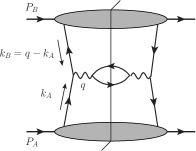
In momentum-space terms, the parton model for DY uses just the graphical structure of Fig. 5. Attached to each incoming hadron is a subgraph dominated by momenta collinear to the hadron. The only connecting lines are the single annihilating parton on each side of the final state cut. However, there are in reality “spectator-spectator” interactions that need to be examined, even though their effects actually cancel in the inclusive cross section. QCD has further non-trivial gluonic effects.

Figure 4: Parton model for DY process in terms of momentum space amplitudes.

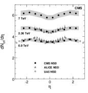
Figure 5: Hadron distribution in pseudo rapidity[5].

3.3 Spectator-spectator interactions

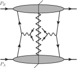
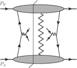
Non-trivial spectator-spectator interactions must exist, because Fig. 5 by itself gives colored particles in the hadronic final states with a large rapidity gap. In contrast the final state in hadron-hadron collisions normally contains hadrons that are distributed approximately uniformly in rapidity: Fig. 5. In Fig. 6, graphs of the form of (a) can fill in the rapidity gap, while graphs like (b) make a reduction in the rapidity-gap cross-section.

(a)	(b)

Figure 6: Structure of simple graphs with final-state interactions. The zigzag line indicates a general graphical structure, often modeled as a sum over ladder graphs or as a pomeron.

The sum over these interactions cancels[6] to leading power in the inclusive cross section. In coordinate space, the cancellation is more intuitive: These interactions happen outside past light-cone of the hard scattering, i.e., too late to affect it. The cancellation only applies to the inclusive DY process: Cross sections in which requirements are imposed on the hadronic final state are a different matter[6].

3.4 Kinematic region of gluons: 1-loop paradigm

Extra terms that affect the TMD factorization formula in QCD are illustrated by Fig. 8, which gives a one-gluon correction to the parton model.

	\psfrag{y}{\small$y_{k}$}\psfrag{yA}{\small$y_{p_{A}}$}\psfrag{yB}{\small$y_{p_{B}}$}\psfrag{ln kT/m}{\small$\ln(k_{\text{T}}/m)$}\psfrag{k-~pB-}{\small$k^{-}\sim p_{B}^{-}$}\psfrag{k+~pA+}{\small$k^{+}\sim p_{A}^{+}$}\psfrag{k-~pB-}{}\psfrag{k+~pA+}{}\includegraphics[scale={0.8}]{figures/split-graph-R}
Figure 7: One real gluon added to parton-model graph.	Figure 8: Region of gluon momentum that is important in Fig. 8.

The relevant kinematic range in the rapidity and the logarithmic transverse momentum of the gluon is shown by the (red) horizontal line in Fig. 8. The gluon approximately has the opposite transverse momentum to the DY pair, and it is emitted essentially uniformly in rapidity, between kinematic limits. The dependence of the rapidity range on $q_{\text{T}}$ is described by the triangle.

Both left- and right-moving gluons are included in the important range of momenta. To obtain factorization, the coupling of a gluon to an oppositely moving quark is converted to a Wilson line vertex in the operator definition of the TMD parton density.

An important consequence, at all orders in gluon emission, is that the $\boldsymbol{q}_{\text{T}}$ distribution becomes energy dependent. Consider Fig. 9,

Figure 9: Effect of boost on gluon in Fig. 8.

which illustrates the effect of increasing $s$ with $x_{A}$ and $x_{B}$ held fixed. At the lower value of $s$, the range of gluon rapidity is the upper thick line. To get to higher $s$, the two incoming hadrons are boosted, in opposite directions. The annihilating quark and antiquark are similarly boosted, because $x_{A}$ and $x_{B}$ are fixed. Left- and right-moving gluons at the lower energy can be similarly boosted, as indicated by the diagonal lines. These effects alone give unchanged transverse momentum. But there is an extra region of gluon emission, in the center at the bottom of the triangle.

The consequent broadening of the transverse-momentum distribution is a definite prediction of QCD. In the CSS-style formalism described below, it appears as an energy dependence of the TMD parton densities.

4 Full factorization

The TMD factorization formula for the cross section in QCD is

$$\frac{\mathop{\mathrm{d}\mskip-0.59999mu\sigma}\nolimits}{\mathop{\mathrm{d}^{4}\mskip-0.59999muq}\nolimits\mathop{\mathrm{d}\mskip-0.59999mu\Omega}\nolimits}$$

$$={} \frac{2}{s}\sum_{j}\frac{\mathop{\mathrm{d}\mskip-0.59999mu\hat{\sigma}_{j\bar{\jmath}}}\nolimits(Q,\mu,g(\mu))}{\mathop{\mathrm{d}\mskip-0.59999mu\Omega}\nolimits}\int\mathop{\mathrm{d}^{2}\mskip-0.59999mu\boldsymbol{b}_{\text{T}}}\nolimits~{}e^{i\boldsymbol{q}_{h\,\text{T}}\cdot\boldsymbol{b}_{\text{T}}}~{}\tilde{f}_{j/A}(x_{A},\boldsymbol{b}_{\text{T}};\zeta_{A},\mu)~{}\tilde{f}_{\bar{\jmath}/B}(x_{B},\boldsymbol{b}_{\text{T}};\zeta_{B},\mu)$$

$$+\mbox{poln.\ terms}+\mbox{high-$q_{\text{T}}$ term}+\mbox{power-suppressed}$$ (2)

where $\mu$ is a renormalization scale, and each $\zeta$ is (up to power corrections) $(2\times\text{corresponding parton energy})^{2}$, with $\zeta_{A}\zeta_{B}=Q^{4}$, e.g., $\zeta_{A}=\zeta_{B}=Q^{2}$. Compared with the parton model formula, (1):

1. The hard scattering, $\mathop{\mathrm{d}\mskip-0.59999mu\hat{\sigma}}\nolimits$ includes higher-order perturbative QCD corrections.

2. The TMD parton densities depend on two auxiliary parameters $\zeta$ and $\mu$.

3. Convolution in $\boldsymbol{q}_{\text{T}}$ is replaced by multiplication in $\boldsymbol{b}_{\text{T}}$.

4. There are similar terms involving polarization-dependence; these are extensively discussed elsewhere in the proceedings of this workshop.

5. TMD factorization is accurate when $q_{\text{T}}\ll Q$. A added correction or matching term using collinear factorization at high $q_{\text{T}}$ gives a formula accurate for all $q_{\text{T}}$.

4.1 Evolution, etc for TMD pdfs

Evolution equations for the TMD parton densities are

$$\frac{\partial\ln\tilde{f}_{f/H}(x,b_{\text{T}};\zeta;\mu)}{\partial\ln\sqrt{\zeta}} =\tilde{K}(b_{\text{T}};\mu),$$ (3)

$$\frac{\mathop{\mathrm{d}\mskip-0.59999mu\ln\tilde{f}_{f/H}(x,b_{\text{T}};\zeta;\mu)}\nolimits}{\mathop{\mathrm{d}\mskip-0.59999mu\ln\mu}\nolimits} =\gamma_{f}(g(\mu);1)-\frac{1}{2}\gamma_{K}(g(\mu))\ln\frac{\zeta}{\mu^{2}},$$ (4)

with provably only a single logarithm of $$\zeta/\mu^{2} \tilde{K}$$ on the right-hand-side of (4). The kernel of the CSS equation (3) obeys

$$\frac{\mathop{\mathrm{d}\mskip-0.59999mu\tilde{K}}\nolimits}{\mathop{\mathrm{d}\mskip-0.59999mu\ln\mu}\nolimits} =-\gamma_{K}\mathopen{}\left(g(\mu)\right).$$ (5)

At small-$b_{\text{T}}$, the TMD parton densities have a generalized operator-product expansion in terms of ordinary parton densities:

$$\tilde{f}_{f/H}(x,b_{\text{T}};\zeta;\mu)=\sum_{j}\int_{x-}^{1+}\frac{\mathop{\mathrm{d}\mskip-0.59999mu\hat{x}}\nolimits}{\hat{x}}\,\tilde{C}_{f/j}\mathopen{}\left(x/\hat{x},b_{\text{T}};\zeta,\mu,g(\mu)\right)\,f_{j/H}(\hat{x};\mu)~{}+~{}O\mathopen{}\left[(mb_{\text{T}})^{p}\right],$$ (6)

where the coefficient functions $\tilde{C}$ are perturbatively calculable.

4.2 Exploit factorization, and evolution

The above equations can be exploited to give predictive power to the formalism.

• Evolution can be used to remove large logarithms in quantities that have an intrinsically large momentum scale.

• Intrinsically non-perturbative parts are in the large $b_{\text{T}}$ behavior of the TMD pdfs and of $\tilde{K}$, and are determined by fits or by non-perturbative calculations/modeling.

4.3 Solutions

I will present two solutions of the equations.

4.3.1 One solution: Factorization with fixed TMD pdfs

In the first, the TMD parton densities appear with fixed scales. This is the closest form to the parton model formula (1), where the parton densities can be treated as intrinsic and universal properties of QCD. The renormalization scale in the hard scattering is chosen of order $Q$, so that it is usefully estimated by a perturbative calculation at low-order.

$$\frac{\mathop{\mathrm{d}\mskip-0.59999mu\sigma}\nolimits}{\mathop{\mathrm{d}^{4}\mskip-0.59999muq}\nolimits\mathop{\mathrm{d}\mskip-0.59999mu\Omega}\nolimits}={} \frac{2}{s}\sum_{j}\frac{\mathop{\mathrm{d}\mskip-0.59999mu\hat{\sigma}_{j\bar{\jmath}}}\nolimits(Q,\mu_{Q},g(\mu))}{\mathop{\mathrm{d}\mskip-0.59999mu\Omega}\nolimits}\int\mathop{\mathrm{d}^{2}\mskip-0.59999mu\boldsymbol{b}_{\text{T}}}\nolimits e^{i\boldsymbol{q}_{h\,\text{T}}\cdot\boldsymbol{b}_{\text{T}}}\times$$

$$\times\tilde{f}_{j/A}\big{(}x_{A},\boldsymbol{b}_{\text{T}};m^{2},\mu_{0}\bigr{)}\,\tilde{f}_{\bar{\jmath}/B}\big{(}x_{B},\boldsymbol{b}_{\text{T}};m^{2},\mu_{0}\bigr{)}$$

$$\times\left(\frac{Q^{2}}{m^{2}}\right)^{\tilde{K}(b_{\text{T}};\mu_{0})}\times\exp\left\{\int_{\mu_{0}}^{\mu_{Q}}\frac{\mathop{\mathrm{d}\mskip-0.59999mu\mu^{\prime}}\nolimits}{\mu^{\prime}}\biggl{[}2\gamma(g(\mu^{\prime});1)-\ln\frac{Q^{2}}{(\mu^{\prime})^{2}}\gamma_{K}(g(\mu^{\prime}))\biggr{]}\right\}$$

$$+\mbox{polarized terms}+\mbox{large $q_{h\,\text{T}}$ correction, $Y$}+\mbox{p.s.c.}$$ (7)

where $\mu_{Q}\propto Q$, while $m$ and $\mu_{0}$ are fixed scales. The scale $\mu_{0}$ should be in a perturbative region, so that anomalous dimensions can be treated perturbatively.

In addition to the TMD parton densities, there is the evolution kernel $\tilde{K}$ (at a fixed scale). This gives a power-law dependence on $Q$, with the power depending on $b_{\text{T}}$. It therefore determines the $Q$ dependence of the shape of the $q_{\text{T}}$ distribution.

4.3.2 Another solution: For maximum perturbative content

The second solution, as presented by CSS[2], has maximum perturbative content: The small-$b_{\text{T}}$ expansion (6) is used when possible, and evolution is applied to its coefficients and to $\tilde{K}$ to remove large logarithms. Remaining non-perturbative content is parameterized by functions to be fit to data.

$$\frac{\mathop{\mathrm{d}\mskip-0.59999mu\sigma}\nolimits}{\mathop{\mathrm{d}^{4}\mskip-0.59999muq}\nolimits\mathop{\mathrm{d}\mskip-0.59999mu\Omega}\nolimits}=\frac{2}{s}\sum_{j,j_{A},j_{B}}\frac{\mathop{\mathrm{d}\mskip-0.59999mu\hat{\sigma}_{j\bar{\jmath}}}\nolimits(Q,\mu_{Q},g(\mu_{Q}))}{\mathop{\mathrm{d}\mskip-0.59999mu\Omega}\nolimits}\int\frac{\mathop{\mathrm{d}^{2}\mskip-0.59999mu\boldsymbol{b}_{\text{T}}}\nolimits}{(2\pi)^{2}}e^{i\boldsymbol{q}_{h\,\text{T}}\cdot\boldsymbol{b}_{\text{T}}}$$

$$\times e^{-g_{j/A}(x_{A},b_{\text{T}})}\int_{x_{A}}^{1}\frac{\mathop{\mathrm{d}\mskip-0.59999mu\hat{x}_{A}}\nolimits}{\hat{x}_{A}}f_{j_{A}/A}(\hat{x}_{A};\mu_{b})~{}\tilde{C}_{j/j_{A}}\mathopen{}\left(\frac{x_{A}}{\hat{x}_{A}},b_{*};\mu_{b}^{2},\mu_{b},g(\mu_{b})\right)$$

$$\times e^{-g_{\bar{\jmath}/B}(x_{B},b_{\text{T}})}\int_{x_{B}}^{1}\frac{\mathop{\mathrm{d}\mskip-0.59999mu\hat{x}_{B}}\nolimits}{\hat{x}_{B}}f_{j_{B}/B}(\hat{x}_{B};\mu_{b})~{}\tilde{C}_{\bar{\jmath}/j_{B}}\mathopen{}\left(\frac{x_{B}}{\hat{x}_{B}},b_{*};\mu_{b}^{2},\mu_{b},g(\mu_{b})\right)$$

$$\times\left(\frac{Q^{2}}{m^{2}}\right)^{-g_{K}(b_{\text{T}})}\left(\frac{Q^{2}}{\mu_{b}^{2}}\right)^{\tilde{K}(b_{*};\mu_{b})}\exp\mathopen{}\left\{\int_{\mu_{b}}^{\mu_{Q}}\frac{\mathop{\mathrm{d}\mskip-0.59999mu\mu^{\prime}}\nolimits}{\mu^{\prime}}\left[2\gamma(g(\mu^{\prime});1)-\ln\frac{Q^{2}}{(\mu^{\prime})^{2}}\gamma_{K}(g(\mu^{\prime}))\right]\right\}$$

$$+\mbox{polarized terms}+\mbox{large-$q_{h\,\text{T}}$ correction, $Y$}+\mbox{p.s.c.}$$ (8)

Here, CSS chose $\boldsymbol{b}_{*}=\ifrac{\boldsymbol{b}_{\text{T}}}{\sqrt{1+b_{\text{T}}^{2}/b_{\rm max}^{2}}}$, with $b_{\rm max}$ a constant chosen so that $\boldsymbol{b}_{*}$ never goes too far beyond the perturbative region. (The appropriateness of choices of $b_{\rm max}$ is under active discussion currently, as can be seen in several other contributions — e.g., those of Boer, Idilbi, Prokudin, and Yuan.) The scale $\mu_{b}$ is proportional to $1/b_{*}(b_{\text{T}})$. Non-perturbative $b_{\text{T}}$ dependence is contained in the functions $g_{j/A}(x_{A},b_{\text{T}})$, $g_{\bar{\jmath}/B}(x_{B},b_{\text{T}})$, and $g_{K}(b_{\text{T}})$.

4.4 Evolution in $q_{\text{T}}$ v. $b_{\text{T}}$

Fig. 10

Low $Q$, $\sqrt{s}$
High $Q$, $\sqrt{s}$

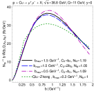
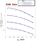
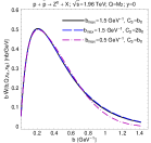
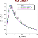
Figure 10: On the left: Integrand[7] in $b_{\text{T}}$ space at low values $Q$ and $s$ and at high values. On the right: corresponding plots[8] for the $q_{\text{T}}$ dependence of the cross section. The plot with CDF data has a zero at $q_{\text{T}}=0$ because the data are given for $\mathop{\mathrm{d}\mskip-0.59999mu\sigma}\nolimits/\mathop{\mathrm{d}\mskip-0.59999muq_{\text{T}}}\nolimits$ instead of $\mathop{\mathrm{d}\mskip-0.59999mu\sigma}\nolimits/\mathop{\mathrm{d}\mskip-0.59999muq_{\text{T}}^{2}}\nolimits$.

shows results for evolution both in $b_{\text{T}}$ space and after Fourier transformation to transverse momentum. As $Q$ increases, the high-$b_{\text{T}}$ tail is strongly suppressed, so a perturbatively-based calculation of the transverse momentum distribution becomes accurate, with the remaining non-perturbative quantitative information being in the ordinary integrated parton densities. The situation is different at relatively low $Q$. Correspondingly the $q_{\text{T}}$ distribution broadens with energy.

5 What form for large $b_{\text{T}}$?

In some standard fits[7, 8], a Gaussian distribution is assumed for the intrinsic transverse-momentum functions, $e^{-\text{const}\times b_{\text{T}}^{2}}$ at large $b_{\text{T}}$. Correspondingly $\tilde{K}$ is assumed to be quadratic in $b_{\text{T}}$ at large $b_{\text{T}}$, which gives an energy dependent Gaussian in the factorization formula: $e^{-\tilde{K}\ln Q^{2}}\sim e^{-\text{const}\times b_{\text{T}}^{2}\ln Q^{2}}$. The coefficients in the Gaussian exponent are substantially non-zero according to the fits in Refs. Konychev:2005iy,Landry:2002ix.

These assumptions should be questioned[9], since Euclidean correlation functions in QFT are usually exponential, $e^{-mb_{\text{T}}}$, not Gaussian at large distances. Furthermore, Schweitzer, Strikman and Weiss[9] argue that there are two relevant non-perturbative scales: a chiral scale $0.3\,\mathrm{fm}=1.5\,\mathrm{GeV^{-1}}$ and a confinement scale = $1\,\mathrm{fm}=5\,\mathrm{GeV^{-1}}$, each with characteristic effects on the sea and valence quark densities. If the scale $m$ is $Q$-independent, then the functions $g_{j/H}(x,b_{\text{T}})$ in Eq. (4.3.2) are linear at large $b_{\text{T}}$, while the function $g_{K}(b_{\text{T}})$ goes to a constant.

In principle the value of $b_{\rm max}$ is irrelevant; any change is compensated by a change in the functional form of the non-perturbative functions. In practice, it is probably preferable to use the information in perturbative calculations as much as possible, so that one should prefer larger values of $b_{\rm max}$. From Ref. Schweitzer:2012hh, it is reasonable that Landry et al’s[8] $b_{\rm max}=0.5\,\mathrm{GeV^{-1}}=0.1\,\mathrm{fm}$ is too low, and that Konychev and Nadolsky’s[7] $1.5\,\mathrm{GeV^{-1}}=0.3\,\mathrm{fm}$ is better. Perhaps an even larger value is sensible. In any case it is probable that the large quadratic terms in the Landry et al fits[8] are mostly reproducing the results of perturbation theory for $b_{\text{T}}$ between about $0.1\,\mathrm{fm}$ and $0.3\,\mathrm{fm}$, rather than giving the true asymptotic behavior at large $b_{\text{T}}$.

In view of the above, I suggest retrying fits with the following forms at large $b_{\text{T}}$:

• $e^{-\text{const}\times b_{\text{T}}}$ in TMD parton densities, with different constants for sea and valence quarks. A possibly useful parameterization for the $e^{-g_{j/H}(x,b_{\text{T}})}$ factor in TMD densities is $e^{-m\left(\sqrt{b_{\text{T}}^{2}+b_{0}^{2}}-b_{0}\right)}$, which is exponential at asymptotically large $b_{\text{T}}$, but approximately Gaussian at relatively small $b_{\text{T}}$.

• $e^{-\tilde{K}\ln Q^{2}}\to e^{-\text{const}\times\ln Q^{2}}$ at large $b_{\text{T}}$ in the evolution factor.

6 Predictions, issues

In principle, the TMD factorization framework is highly predictive (and hence testable). Basically, one can fit the non-perturbative $b_{\text{T}}$-dependence of TMD functions at low energy. The dependence of one process on $Q$, for a limited range of $Q$ with fixed $x$ is sufficient to fit the non-perturbative $\tilde{K}$. Then everything else is predicted. Using polarized TMD parton densities and fragmentation functions does not need new values of $\tilde{K}$. There is also the predicted sign reversal of naively T-odd TMD parton densities (the Sivers function, etc) between DY and SIDIS.

The standard processes are (a) DY, sensitive to TMD parton densities in certain combinations; (b) SIDIS, sensitive to both TMD parton densities and fragmentation functions, in many flavor combinations; (c) $e^{+}e^{-}\to\text{back-to-back hadrons}$, sensitive to TMD fragmentation functions, including flavor dependence.

Given the recent extra data, especially at relatively low $Q$, and given the issues about the functional form of the non-perturbative $b_{\text{T}}$ dependence, it is important to update global fits beyond Refs. Konychev:2005iy,Landry:2002ix. In addition, as can be seen from other contributions to this workshop, there is an urgent need to reconcile treatments.

Finally, note the predicted violation of TMD factorization in hadro-production of hadrons — see, for example, the contribution of Rogers for new work. Much work here is needed; it is an important source of new phenomena in QCD. Fits to data where TMD factorization is valid are important in quantitatively assessing factorization breaking elsewhere.

References

• [1] J.Β C. Collins and D.Β E. Soper, Nucl. Phys., B193, 381–443, 1981. Erratum: B213, 545 (1983).
• [2] J.Β C. Collins, D.Β E. Soper, and G.Β Sterman, Nucl. Phys., B250, 199–224, 1985.
• [3] J.Β C. Collins. Foundations of Perturbative QCD (Cambridge University Press, Cambridge, 2011).
• [4] S.Β D. Drell and T.-M. Yan, Phys. Rev. Lett., 25, 316–320, 1970.
• [5] V.Β Khachatryan etΒ al., Phys. Rev. Lett., 105, 022002, 2010.
• [6] C.Β E. DeTar, S.Β D. Ellis, and P.Β V. Landshoff, Nucl. Phys., B87, 176, 1975.
• [7] A.Β V. Konychev and P.Β M. Nadolsky, Phys. Lett., B633, 710–714, 2006.
• [8] F.Β Landry, R.Β Brock, P.Β M. Nadolsky, and C.-P. Yuan, Phys. Rev., D67, 073016, 2003.
• [9] P.Β Schweitzer, M.Β Strikman, and C.Β Weiss, JHEP, 1301, 163, 2013.