Redshift Space Distortion Reconstruction

Abstract

Redshift space distortions of the matter density power spectrum carry information on the growth rate of cosmic structure but require accurate modeling of nonlinear and velocity effects on the density field. We test and advance the reconstruction function of Kwan, Lewis, Linder (2012) in several ways. First, we compare to the distribution function perturbative approach of Seljak & McDonald (2012), deriving the mapping between them and showing how the KLL form can extend the validity of the latter. Second, using cosmological simulations rather than perturbation theory we calibrate the free functions within the KLL reconstruction form and fit their behavior in redshift and wavenumber. An efficient, new analysis pipeline rapidly calculates from simulation outputs the redshift space power spectrum. The end result is a robust analytic reconstruction function mapping the linear, real space matter power spectrum to the nonlinear, anisotropic redshift space power spectrum to an accuracy of $\sim$2-5% in the range $k=0.1-0.5\,h$/Mpc for $z=0-2$. As a by-product we derive RealEasy, an analytic mapping to the nonlinear, real space matter power spectrum (i.e. an analog to Halofit) to $\sim 1\%$ accuracy over the same range. We also investigate an approach converse to KLL and find it to be complementary and capable of achieving an accuracy of $\sim$2-4% over the range $k=0.3-1\,h$/Mpc for $z=0-2$.

I Introduction

Three dimensional maps of galaxy clustering in large volumes of our Universe are becoming viable with the current and next generation of spectroscopic surveys (e.g. BOSS boss , DESI desi , PFS pfs ). These carry abundant, detailed information on the growth of large scale structure and the cosmological and astrophysical parameters affecting that structure. In particular, since observations deliver information in redshift space, the data is a function of both the matter density and velocity field. Nonlinear clustering amplifies the linear power on small scales, while velocities induced by mass inhomogeneities cause redshift space distortions that turn the real space power spectrum anisotropic.

Thus observations are of the nonlinear, anisotropic redshift space power spectrum though theory is most adept at relating cosmological parameters to the linear, isotropic real space power spectrum. In order to extract the cosmological information from the data we require robust maps between them. Many methods have been devised for carrying out this transformation kaiser ; matsza ; scocci ; taruya ; tang ; reidwhite ; jennings , most relying on extending perturbation theory beyond the linear density regime. Here we explore two more general prescriptions: the reconstruction function approach of kll and the distribution function method of smd1 .

The reconstruction function approach fits an analytic corrector function to the ratio between computational simulation results for the fully nonlinear redshift space density power spectrum and the linear real space density power spectrum, carrying out the mapping all in one step. The derived reconstruction form, hereafter called KLL, can be physically motivated as combinations of nonlinear and velocity effects. It has been shown to be highly accurate, even out to wavenumbers $k=1\,h$/Mpc for dark matter and $k=0.6\,h$/Mpc for halos kll ; julithesis . The KLL form has a fixed angular dependence but relies on simulations to determine the wavenumber $k$ and redshift $z$ dependence of its three free coefficients.

The distribution function approach uses perturbation theory to expand the redshift space power spectrum in moments of the phase space distribution. Its form, hereafter called SMD, builds up from the linear theory in a perturbation sum and so is highly predictive but its accuracy breaks down as the wavenumber quantity used in the expansion moves outside its realm of validity.

Here we explore the relation of these two approaches, combining the best features of each, and how simulations can further improve the reconstruction. In Sec. II we derive the mapping from one approach to the other, compare the results of each to simulations, and consider their combination. Section III uses simulations rather than perturbation theory to calibrate and investigate the redshift and wavenumber dependence of the KLL coefficients, and test the accuracy of its reconstruction. Using these results we give an analytic fit to the real space power spectrum in Sec. LABEL:sec:real and discuss an alternate redshift space approach in Sec. IV. We summarize and conclude in Sec. V.

II Mapping between KLL Reconstruction and SMD Perturbation Theory

Nonlinear structure formation maps a linear power spectrum at some redshift $z$ to a nonlinear power spectrum at $z$. Redshift space distortions add a contribution due to the velocities along the line of sight, causing anisotropy with respect to the wavenumbers parallel to the line of sight, $k_{\parallel}=k\mu$, and perpendicular to the line of sight, $k_{\perp}=k\sqrt{1-\mu^{2}}$, where $\mu$ is the cosine of the wavevector with respect to the line of sight.

II.1 KLL reconstruction function

The KLL approach uses a reconstruction function $F(k,\mu,z)$ operating on some model for the power spectrum to give the full nonlinear, anisotropic redshift space power spectrum,

$$P(k,\mu,z)=F(k,\mu,z)\,P_{\rm model}(k,\mu,z)\ .$$ (1)

The quantity $P(k,\mu,z)$ is sometimes written in the literature as $P^{s}$. The KLL form fitted to simulations in kll is

$$F(k,\mu,z)=\frac{A(k,z)}{1+B(k,z)\,k^{2}\mu^{2}}+C(k,z)\,k^{2}\mu^{2}\ ,$$ (2)

where the coefficients depend on the model to be corrected. For example one could take $P_{\rm model}$ to be the linear real space power spectrum or some more complex prediction from higher order perturbation theory.

We choose as $P_{\rm model}$ the linear theory redshift space power spectrum, i.e. the Kaiser formula

$$P_{\rm Kaiser}(k,\mu,z)=[b(z)+f(z)\mu^{2}]^{2}\,P_{L}(k,z)\ ,$$ (3)

where $P_{L}$ is the linear real space power spectrum, $f$ is the linear growth rate, and $b$ is the tracer (e.g. galaxy) bias. While any model can be corrected accurately (see, e.g., kll for examples using the models of scocci ; taruya ), the Kaiser formula is correct in the limit of small wavenumber and is simply calculated. Rather than doing a partial correction through higher order perturbation theory and another correction through $F$, we use the KLL form to account for the entire reconstruction.

II.2 SMD distribution function

Another approach, defined in smd1 and investigated further in smd2 ; smd3 ; smd4 , begins by considering the distribution function of particles in phase space $f(\vec{x},\vec{q},t)$. The dynamics of the system is controlled by the Vlasov-Poisson equation describing the evolution of $f(\vec{x},\vec{q},t)$. Since particles in a simulation are supposed to sample $f(\vec{x},\vec{q},t)$, this approach is appealing both theoretically and practically, as it can be translated straightforwardly into prescriptions to carry out measurements on N-body simulations (see smd2 ).

This formalism is based on introducing the following $n$-rank tensors

$$T^{n}_{i_{1},i_{2},...,i_{n}}(\vec{x}) \equiv \frac{m}{\bar{\rho}}\int d^{3}\vec{q}\,f(\vec{x},\vec{q})\,u_{i_{1}}\,u_{i_{2}}\,...u_{i_{n}}$$ (4)

$$T^{n}_{i_{1},i_{2},...,i_{n}}(\vec{k}) = \int d^{3}\vec{x}\,e^{i\vec{k}\cdot\vec{x}}T^{n}_{i_{1},i_{2},...,i_{n}}(\vec{x})\ ,$$ (5)

where $\vec{q}=m\vec{u}$ is the comoving momentum. The density field in redshift space is then written as

$$\delta_{s}(\vec{k})=\sum_{n}\frac{1}{n!}\left(\frac{ik\mu}{aH}\right)^{n}\,T_{\parallel}^{n}(\vec{k})\ .$$ (6)

By defining $P^{ab}(\vec{k})\delta_{D}(\vec{k}-\vec{k^{\prime}})\equiv\langle T_{\parallel}^{a}(\vec{k})T_{\parallel}^{*b}(\vec{k})\rangle$ the redshift space power spectrum gets expressed as

$$P(\vec{k}) = \sum_{n=0}^{\infty}\frac{1}{(n!)^{2}}\left(\frac{k\mu}{aH}\right)^{2n}\,P^{nn}(\vec{k})$$ (7)

$$+ 2\,{\rm Re}\left[\sum_{a=0}^{\infty}\sum_{b>a}^{\infty}\frac{(-1)^{b}}{a!b!}\left(\frac{ik\mu}{aH}\right)^{a+b}P^{ab}(\vec{k})\right].$$

At the same time, the angular dependence of the $T_{\parallel}^{n}(\vec{k})$ tensors can be expressed using spherical harmonics,

$$T_{\parallel}^{n}(\vec{k})=\sum_{l=n,n-2...}^{0\textrm{ or }1}\sum_{m=-l}^{l}C_{lm}T_{lm}^{n}(k)Y_{lm}(\theta,\phi)\ ,$$ (8)

where $C_{lm}$ are normalization constants. Each $P^{ab}$ can then be expressed as a combination of these terms. Note that two sets of $l$’s and $m$’s will appear, belonging to the two $T_{\parallel}$’s that are being correlated. However when averaging over the azimuthal angle $\phi$ all the terms with $m\neq m^{\prime}$ will vanish. This then implies that

$$P^{ab}(\vec{k}) = \sum_{l=a,a-2,\dots}^{0\textrm{ or }1}\ \sum_{l^{\prime}=b,b-2,\dots}^{0\textrm{ or }1}$$

$$\sum_{m=0}^{{\rm min}(l,l^{\prime})}\,P_{ll^{\prime}m}^{ab}(k)\mathcal{P}_{lm}(\mu)\,\mathcal{P}_{l^{\prime}m}(\mu)$$

where $\mathcal{P}_{lm}$ denotes the associated Legendre polynomials.

Thus the power spectrum is built up out of a momentum moment expansion in terms of 2-index power spectra $P^{ab}(\vec{k})$, and these in turn are constructed from an angular expansion involving 5-index power spectra $P_{ll^{\prime}m}^{ab}(k)$. Note that this formulation cleverly allows separation of the $k$ and $\mu$ dependence of the $P^{ab}$. Once the $P_{ll^{\prime}m}^{ab}(k)$ are computed or measured, all the rest follow.

It is useful to write down a few of the $P^{ab}$ appearing in Eq. (II.2):

$$P^{00}(\vec{k}) = P_{000}^{00}$$ (10)

$$P^{01}(\vec{k}) = P_{010}^{01}\mu=-\frac{i\mu}{2k}\frac{dP^{00}(k)}{dt}$$ (11)

$$P^{11}(\vec{k}) = P_{110}^{11}\mu^{2}+P_{111}^{11}(1-\mu^{2})$$ (12)

$$= \mu^{2}(P_{110}^{11}-P_{111}^{11})+P_{111}^{11}$$

$$P^{02}(\vec{k}) = P^{02}_{000}-\frac{P^{02}_{020}}{2}+\frac{3\mu^{2}}{2}P^{02}_{020}$$ (13)

$$P^{12}(\vec{k}) = P^{12}_{120}\left(\frac{3\mu^{3}-\mu}{2}\right)+P_{121}^{12}3\mu\left(1-\mu^{2}\right)$$ (14)

$$P^{22}(\vec{k}) = \mu^{4}\left(\frac{9P_{220}^{22}}{4}-9P_{221}^{22}+9P_{222}^{22}\right)$$ (15)

$$+ \mu^{2}\left(9P_{221}^{22}-\frac{3P_{220}^{22}}{2}-18P_{222}^{22}+\frac{3P_{020}^{22}}{2}\right)$$

$$+ \frac{P_{220}^{22}}{4}+P_{000}^{22}-\frac{P_{020}^{22}}{2}+9P_{222}^{22}$$

$$P^{03}(\vec{k}) = \mu\,P_{010}^{03}+\frac{P_{030}^{03}}{2}\left(5\mu^{3}-3\mu\right)$$ (16)

$$P^{13}(\vec{k}) = P_{111}^{13}-\frac{3}{2}P_{131}^{13}+\mu^{4}\left(\frac{5}{2}P_{130}^{13}-\frac{15}{2}P_{131}^{13}\right)$$ (17)

$$+ \mu^{2}\left(P_{110}^{13}-P_{111}^{13}-\frac{3}{2}P_{130}^{13}+9P_{131}^{13}\right)$$

$$P^{04}(\vec{k}) = P_{000}^{04}-\frac{P_{020}^{04}}{2}+\frac{3P_{040}^{04}}{8}+\frac{35\mu^{4}}{8}P_{040}^{04}$$ (18)

$$+ \mu^{2}\left(\frac{3}{2}P_{020}^{04}-\frac{30}{8}P_{040}^{04}\right)$$

Now recall the definition of $P^{ab}_{ll^{\prime}m}$ as a correlator of $T_{\parallel}$’s. That is,

$$P^{ab}_{ll^{\prime}m}(k)\,\delta(k-k^{\prime})\equiv\langle T^{a}_{lm}(k)\,T^{*b}_{l^{\prime}m^{\prime}}(k^{\prime})\rangle\delta_{mm^{\prime}}\ .$$ (19)

The physical meaning of the different terms contributing to the 5-index $P^{ab}_{ll^{\prime}m}$ can be identified as correlations of the density/velocity/stress-energy (given by the index $a$) with density/velocity/stress-energy (given by the index $b$).

II.3 Angular dependence comparison

The redshift space power spectra predicted by the KLL reconstruction function (times the Kaiser formula) can be directly compared to that from the SMD distribution function approach by identifying terms with common angular dependence, i.e. $\mu^{0}$, $\mu^{2}$, $\mu^{4}$, etc. If one instead tries to compare terms with common $k$ dependence, one breaks the definition of $f$ as the linear growth rate and forces it to become $k$ dependent; furthermore the $k$ dependence of the $A$, $B$, $C$ coefficients is not known a priori – this will be informed by the mapping.

Within SMD, all $k$ dependence is separated from the angular $\mu$ dependence so one can write

$$P(k,\mu) = \sum_{n=0}^{\infty}\mu^{2n}\,\sum_{\alpha}S_{n\alpha}(k)=\sum_{n=0}^{\infty}\mu^{2n}\,\bar{P}_{2n}(k)\,,$$ (20)

where $\alpha$ is a generic index that gathers together $l$, $l^{\prime}$, etc., $S$ condenses the non-angular factors in Eq. (7), and $\bar{P}_{2n}$ further simplifies the sum. Of course since SMD relies on a perturbative expansion, this formalism will break down past some region of validity.

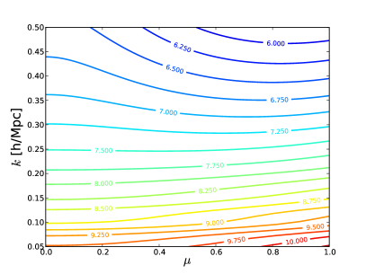
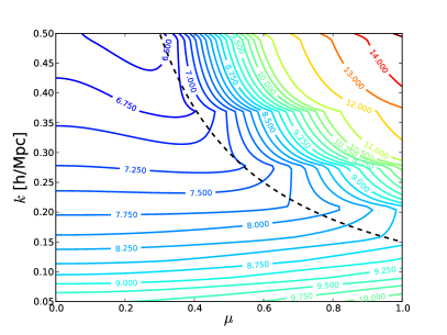
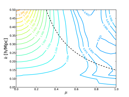
Figure 1 plots the logarithm of the redshift space power spectra in the $k$–$\mu$ plane, for the KLL (left panel) and SMD (right panel) cases. We work at redshift $z=0$ as the greatest challenge to accurate modeling. Three characteristics are apparent: 1) Good agreement in the linear region ($k\ll 1$), 2) Good agreement at small angles to the line of sight ($\mu\ll 1$), and 3) Breakdown of SMD beyond $k\mu\gtrsim 0.15\,h$/Mpc. This limit to the SMD approach agrees with that reported in smd2 . We emphasize that the KLL results shown come purely from the analytic prediction using the coefficients given in linsam , with no adjustable parameters (linsam roughly estimated the coefficients; we will calibrate them using a simulation analysis pipeline later in this paper).

Figure 1: Isocontours of the redshift space power spectra ($\ln P$) are shown for the KLL approach (left panel) and for the SMD approach (right panel). The two methods agree for small $k\mu$ and KLL is known to match numerical simulations, but the SMD approach breaks down around $k\mu\gtrsim 0.15\,h$/Mpc (given by the dashed curve).

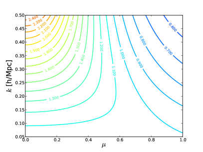
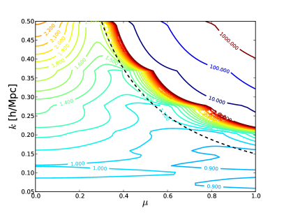
As an alternate view, we show in Fig. 2 the reconstruction functions necessary to take the linear real space power spectrum to the predicted nonlinear redshift space power spectrum in each approach. We see that this correction in the SMD case runs away to large values for $k\mu\gtrsim 0.15\,h$/Mpc.

Figure 2: Reconstruction (“corrector”) functions for the KLL (left) and SMD (right) formalisms are shown in the $k$–$\mu$ plane.

While keeping in mind the range of validity, we can now proceed to the comparison of KLL and SMD term by term in the $\mu^{n}$ expansion. For the terms independent of $\mu$ (i.e. isotropic), equating the terms implies

$$P_{L}(k)\,A(k)=\bar{P}_{0}(k)=P_{NL}(k)\ ,$$ (21)

where $P_{NL}$ is the nonlinear real space power spectrum, so $A$ is just the ratio of the nonlinear to linear isotropic power spectra, as also found by kll .

The next two terms, depending on $\mu^{2}$ and $\mu^{4}$, give

$$2fP_{L}\,A+K^{2}P_{L}\,(C-AB)=\bar{P}_{2}$$ (22)

$$f^{2}P_{L}+2K^{2}fP_{L}\,(C-AB)+K^{4}AB^{2}P_{L}=\bar{P}_{4}$$ (23)

where $K\equiv k/(aH)$. The quantities $B$ and $C$ are mixed together, involving the autocorrelations of the first moment of the phase space distribution, i.e. the velocity field, but also nonlinearities and cross-correlations in the density and the stress-energy (see also smd2 ; kll ).

Figure 3: The reconstruction function is shown for coefficients constructed using Eqs. (24-26) and measurements from the simulations of smd2 but using the KLL form. This successfully removes the dramatic breakdown seen in the right panel of Fig. 2.

Solving these three equations for $A$, $B$, and $C$ yields the mapping between the two approaches:

$$A = \frac{P_{NL}}{P_{L}}$$ (24)

$$B^{2} = \frac{\bar{P}_{4}-2f\bar{P}_{2}}{K^{4}\,P_{NL}}+3\frac{f^{2}}{K^{4}}$$ (25)

$$C = AB+\frac{\bar{P}_{2}-2fP_{NL}}{K^{2}\,P_{L}}\ .$$ (26)

Thus $\bar{P}_{0}$, $\bar{P}_{2}$, $\bar{P}_{4}$ can be determined by $A$, $B$, and $C$ through Eqs. (21)–(23), or conversely $A$, $B$, and $C$ can be found by Eqs. (24)–(26). Also note that the coefficients always enter in KLL as $BK^{2}$ and $CK^{2}$.

At higher orders, since $A$, $B$, $C$ are already determined, the KLL terms will differ in general from the moment method expansion terms. (Note that KLL implicitly includes all orders of $\mu$.) However, the higher order SMD terms are negligible except at $k>0.1\,h$/Mpc smd2 and SMD quickly loses accuracy at higher $k$. So the mapping we have established is sufficient.

Indeed we can use this mapping to merge the strengths of each approach: the physical basis at low $k\mu$ of the perturbation theory in SMD with the analytic reconstruction over a wide range of $k\mu$ in the KLL form. In the next section we apply this by deriving $A$, $B$, $C$ from the SMD 2-index power spectra of their simulations (rather than using the values in linsam ), then feeding these into the KLL reconstruction form and comparing to the full nonlinear redshift space power spectrum of the simulation. We will see this use of the KLL form significantly extends the range of accuracy of the reconstruction.

Figure 4: KLL coefficient functions $A(k)$, $B(k)$, and $C(k)$ as measured from the M000 model of the Coyote Universe simulation suite are plotted for $z=\{0,0.11,0.25,0.43,0.67,1,1.5,2\}$, from top to bottom for $A$, bottom to top for $C$, and as labeled for $B$. The red, dashed lines are simple analytic fits.

II.4 Applying the mapping

Summing the measurements of $P^{ab}$ (kindly provided to us by Teppei Okumura) on the simulations in smd2 , we can get the terms $\bar{P}_{2n}$. From these, Eqs. (24)–(26) provide $A$, $B$, and $C$. Those coefficients are then used within the usual KLL reconstruction function to transform the linear power spectrum $P_{L}$ (and the Kaiser formula) into a predicted nonlinear redshift space power spectrum.

The derived reconstruction function is shown in Fig. 3. Comparing to the right panel of Fig. 2, the original SMD approach, we see a marked improvement, with no sign of the cliff beyond $k\mu\gtrsim 0.15\,h$/Mpc where the SMD function jumps upward by a factor of a thousand. Rather, the reconstruction is now much smoother and in qualitative accord with the pattern of the left panel of Fig. 2, the baseline KLL approach. There is no obvious breakdown in going to higher $k\mu$, one of the virtues of the KLL method’s implicit inclusion of all orders of $\mu$.

These results highlight the power of both the KLL form and the advantage of using simulations to estimate accurately the coefficients $A(k,z)$, $B(k,z)$, $C(k,z)$. In the next section we leave perturbation theory behind and develop an efficient computational pipeline to extract from simulations accurate fits for $A$, $B$, and $C$. We apply this to a high definition realization of the Coyote cosmological simulation suite as an example.

III Calibrating KLL Coefficients with Simulations

In order to calibrate the KLL coefficients from cosmological simulations we have developed a parallel MPI code that, starting from a simulation snapshot, computes the redshift space power spectrum and fits the reconstruction coefficients as a function of $k$ at each redshift. This automated analysis pipeline is flexible enough to handle large simulation boxes. As is often the case, the limiting factor in this analysis is the amount of memory per rank: since the FFT is carried out by decomposing the simulation box into slabs and assigning each slab to a rank, the largest number of cells into which the snapshot can be decomposed is determined by the amount of memory required for a single layer slab (i.e. a 3D slab of dimensions $N\times N\times 1$, where N is the number of cells the snapshot is decomposed into).

The operations carried out on the data ranks have been decomposed into a set of simple “atomic” operations – while this choice might seem an extra complication, this allows the implementation of other kinds of analyses using the same framework. In particular, the implementation of the measurement of the SMD power spectra $P^{ab}(\vec{k})$ and of the divergence of the velocity field, if desired, become straightforward. Furthermore, the implementation of the particle deposition scheme is flexible enough to allow reconstructing the density field starting from “particles” of different masses; within this framework it is therefore straightforward to carry out measurements also using halos (although we leave this for future work).

Figure 5: Fractional difference between the RSD power spectrum measured on M000 simulation and the one reconstructed using the best fit calibrated values of $A(k)$, $B(k)$, and $C(k)$, at $z=0$, 0.67, 2 (top, center, bottom panel).

Briefly, the steps taken to carry out the measurement and fit are:

1. Load the particles and, if calculating the redshift space distorted density field, displace them according to their velocity along a predetermined direction that has been chosen as the line of sight.

2. Reconstruct the density field $\delta(\vec{x})$ on a 3D grid using a cloud in cell deposition scheme.

3. Fourier transform the density field and deconvolve the cloud in cell deposition scheme to obtain $\delta(\vec{k})$.

4. Square the Fourier transformed density field.

5. Bin the results in both $\{k_{\perp},k_{\parallel}\}$ and $\{k,\mu\}$ and thus measure the power spectra.

6. Measure $F(k,\mu)$ from

   $$F(k,\mu,z)=\frac{P(k,\mu,z)}{P_{L}(k,\mu,z)[1+f(z)\mu^{2}]^{2}},$$ (27)

   where for the linear power spectrum we use the one measured on the initial conditions, multiplied by appropriate linear growth to redshift $z$.

7. For each bin in $k$-space $k_{i}$ and each redshift $z_{j}$ we then find the best fit value for $A(k_{i},z_{j})$, $B(k_{i},z_{j})$ and $C(k_{i},z_{j})$.

As a first application, we use our analysis pipeline on the high resolution box of the M000 model of the Coyote Universe simulation suite Heitmann:2008eq ; Heitmann:2009cu ; Lawrence:2009uk : a flat $\Lambda$CDM cosmology with dimensionless physical matter density $\omega_{m}=0.1296$, physical baryon density $\omega_{b}=0.0224$, scalar tilt $n_{s}=0.97$, amplitude of mass fluctuations today $\sigma_{8}=0.8$, and reduced Hubble constant today $h=0.72$ containing $1024^{3}$ dark matter particles in a box of 1300 Mpc evolved starting from $z=200$ using the publicly available code GADGET-2.

Having access only to the high resolution realization of the Coyote Universe suite restricts the accuracy with which the power spectrum can be measured on large scales. The fractional precision is approximately given by the inverse square root of the number of measurable modes, thus

$$\frac{\delta P}{P} \approx N_{\rm modes}^{-1/2}=\left(\frac{3}{2}\frac{k^{2}\Delta k\Delta\mu V_{\rm box}}{4\pi^{2}}\right)^{-1/2}$$ (28)

$$\approx 1.61\left(\frac{k}{0.25}\right)^{-1}\left(\frac{\Delta k}{0.04}\right)^{-1/2}\left(\frac{\Delta\mu}{0.05}\right)^{-1/2}\%\$$ (29)

where the 3 in the $3/2$ reflects the 3 orthogonal directions through the box and the 2 comes from using the real part of the Fourier modes. We have verified the results through actual mode counting.

Currently, we restrict our analysis to the regime where the simulation scatter $\delta P/P\lesssim 2\%$, since that will be our reconstruction accuracy goal, corresponding to $k\gtrsim 0.25\,h$/Mpc. We regard this investigation as a proof of principle, since given success here there should be no substantial obstacle to increasing its precision through multiple realizations, extending its range to larger scales (smaller $k$), and connecting it down to the perturbation theory region. On the high $k$ end (small scales), we will explore out to $k_{\rm max}=0.5\,h$/Mpc, although our reconstruction function works reasonably beyond this. The analytic fits we discuss next are therefore applied to the range $k=0.25-0.5\,h$/Mpc.

We optimize the reconstruction function coefficients so as to minimize the residuals of the redshift space power spectrum relative to the simulation results over the $k$-$\mu$ space. We adopt $\Delta k=0.04$ and $\Delta\mu=0.05$ and have also checked that the joint $k$-$\mu$ optimization is consistent with a $\mu$ optimization at each fixed $k$.

Figure 6: Fractional difference between the RSD power spectrum measured on M000 simulation and the one using the simple analytic reconstruction from Eqs. (30), (33), (34), at $z=0$, 0.67, 2 (top, center, bottom panel).

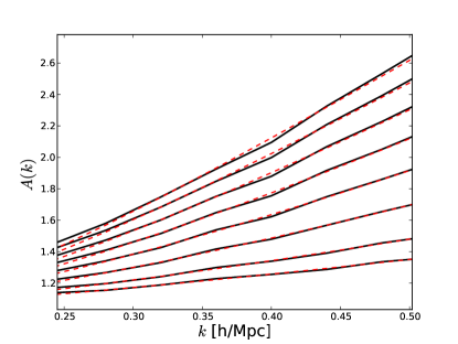
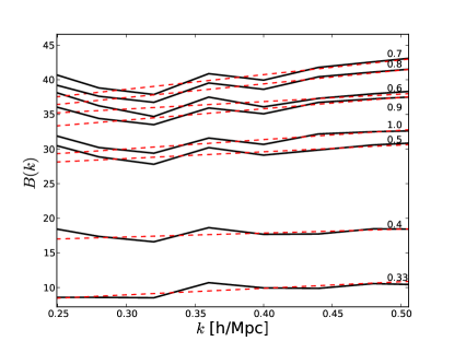
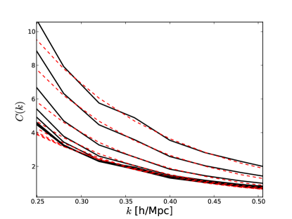
The best fit functions $A(k)$, $B(k)$ and $C(k)$ obtained for $a=\{1,0.9,0.8,0.7,0.6,0.5,0.4,0.333\}$, i.e. $z=\{0,0.11,0.25,0.43,0.67,1,1.5,2\}$ are shown in Fig. 4. We find the reconstruction function coefficients are well behaved, with simple forms in $k$ and somewhat more complicated dependence on redshift. We discuss each coefficient in turn. The deviation of the factor $A(k,z)$ from unity arises from nonlinearity and so as expected $A$ increases with $k$ and decreases with redshift (increases with $a$). The quantity $B$ acts like a velocity dispersion, including nonlinear effects, and as expected is small at large redshift, increasing as nonlinearity does. However, the velocity effects also decline toward the present as the growth rate $f$ does as dark energy comes to dominate – recall that the velocity damping often enters in the combination $f^{2}\sigma_{v}^{2}k^{2}\mu^{2}$ (cf. $Bk^{2}\mu^{2}$ in KLL). These competing factors cause $B$ to be nonmonotonic with redshift, reaching a maximum amplitude around $z\approx 0.6$. The $k$ dependence of $B$, however, is small over this range, with a slight linear trend out to $k\approx 0.8\,h$/Mpc. The coefficient $C$ also involves a mix of velocity and nonlinear effects, and acts to restore some power lost to the damping. This quickly dies off (roughly exponentially) with $k$, however, and also with decreasing redshift.

Figure 7: Isocontours of the nonlinear, redshift space power spectrum measured on the M000 simulation are plotted in the $k$-$\mu$ plane. The color bar shows the log of the power spectrum.

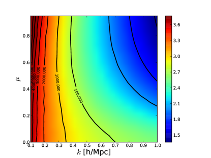
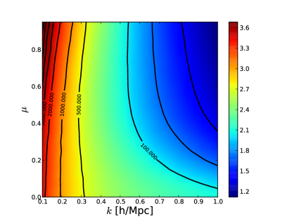
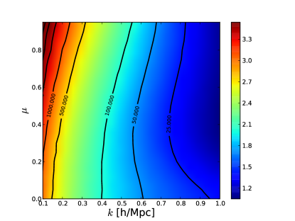
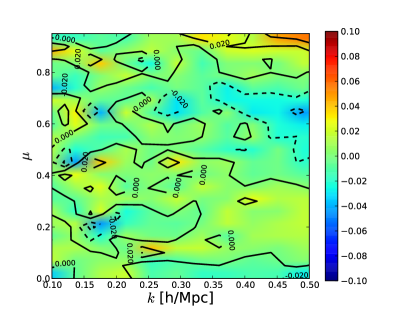
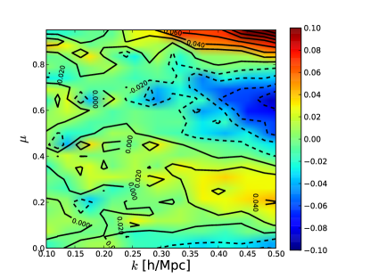
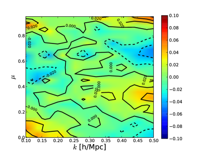
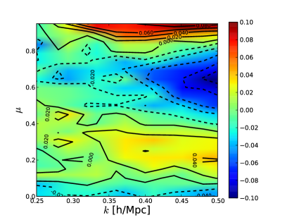
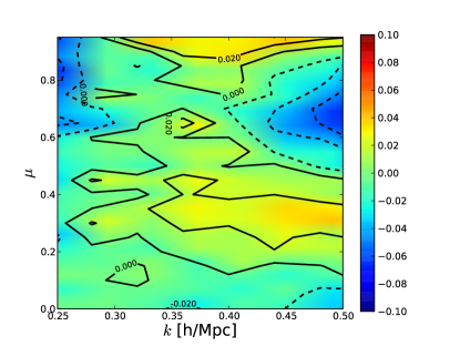
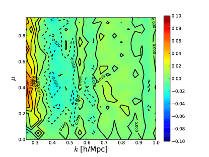
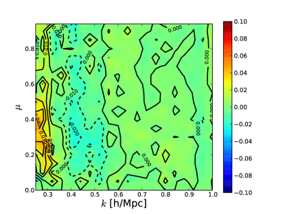
Figure 5 shows the fractional difference between the simulation measurement and the full, calibrated KLL result. The calibrated reconstruction is accurate at the 2% level at low redshift and high redshift, with limited regions of the $k$-$\mu$ plane having $\gtrsim 5\%$ deviations around $z\approx 1$. This appears to be due to the interplay of velocity and nonlinear density effects being comparable at that epoch. Overall, the reconstruction of the simulated nonlinear redshift space power spectrum shows that the KLL form provides a good description over this range of $k$ and $z$.

Given the simple behaviors of the coefficients seen in Fig. 4, we can explore purely analytic fits for the reconstruction function. For full calculations one should use the calibrated coefficients, but for quick if approximate results it is of interest to see how well the analytic approximations perform. We adopt

$$A=\left[1+\left(\frac{k}{k_{A}}\right)^{n}\,\right]^{1/n}\ ,$$ (30)

where this form gives a power law increase above 1 at low $k$ and then matches at higher $k$ the linear dependence on $k$ observed in the simulation results. Table 1 gives the values for $k_{A}$ and $n$ at each scale factor, but these approximately follow

$$k_{A}(a) \approx 0.194+(1-a)^{2.4}$$ (31)

$$n(a) \approx 3.2-2.54(1-a)\ .$$ (32)

For $B$, the $k$ dependence is linear over a wide range, so we adopt

$$B=B_{0}+B_{1}k\ ,$$ (33)

and give the values for $B_{0}(a)$ and $B_{1}(a)$ in Table 1. Similarly for $C$ the exponential $k$ dependence is a good approximation, with

$$C=C_{0}\,e^{-k/k_{C}}\ ,$$ (34)

and the values for $C_{0}(a)$ and $k_{C}(a)$ are in Table 1.

$a$	$k_{A}$	$n$	$B_{0}$	$B_{1}$	$C_{0}$	$k_{C}$
0.333	0.75	$\ 1.47\$	$\ 6.09\$	$\ 9.47\$	$\ 46.0\$	$\ 6.34\$
0.4	0.52	1.68	15.6	5.67	44.9	7.07
0.5	0.37	1.94	25.7	9.79	37.1	7.45
0.6	0.30	2.17	32.5	10.8	29.6	7.43
0.7	0.25	2.42	32.2	21.2	26.8	7.41
0.8	0.23	2.64	31.5	19.8	24.4	7.24
0.9	0.21	2.87	29.3	16.4	22.2	6.95
1.0	0.19	3.23	$\ 26.0\$	$\ 13.5\$	19.7	6.54

Table 1: The parameter values for the redshift space power spectrum fits of Eqs. (30-34) at each scale factor $a$, with $k_{A}$ and $k_{C}$ in units of $h$/Mpc, $B_{0}$ and $C_{0}$ in $({\rm Mpc}/h)^{2}$, $B_{1}$ in $({\rm Mpc}/h)^{3}$, and $n$ dimensionless.

These expressions capture the $k$ dependences and do well quantitatively at reproducing the coefficient values over the range $k=0.25-0.5\,h$/Mpc and $z=0-2$. The true test, however, is how well the reconstructed nonlinear redshift space power spectrum matches the truth measured from the simulations.

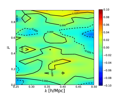
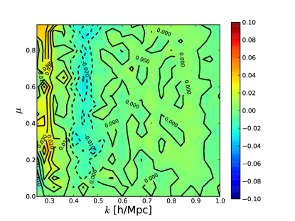
Figure 6 shows the fractional difference between the simulation measurement and the purely analytic KLL result. We see that the analytic approximation does nearly as well as the calibrated coefficients in the fit range of $k=0.25-0.5\,h$/Mpc. Appendix A considers the accuracy for fits to the real space power spectrum.

IV Converse Approach

The KLL form has demonstrated successful reconstruction of redshift space distortions by adopting a functional form for the angular dependence $\mu$ and fitting for the $k$ dependence. One might imagine the converse approach of adopting a functional form for the $k$ dependence and fitting for the $\mu$ dependence. Remarkably this shows promise as well, and we briefly describe this VL method, leaving its development for future work.

Part of the reason why this is possible is the smoothness of the redshift space power spectrum. Figure 7 shows the redshift space power spectrum measured from the M000 simulation at three redshifts. The isocontours of the power spectrum are smooth curves in the $k$-$\mu$ plane, gradually changing with redshift, so simple functional forms can accurately capture their behavior.

The nonlinear real space power spectrum is a $k$-dependent but $\mu$-independent amplification of the linear power spectrum; let us assume this is determined directly by simulations and concentrate on the redshift space distortion effects. We write these as

$$P(k,\mu,z)=e^{-(Ek^{2}+Fk+G)}\,P^{r}(k,z)\ ,$$ (35)

where the VL reconstruction coefficients $E,F,G$ are all functions of $\mu$ and $z$.

This approach allows general angular dependence, but its $k$ dependence is determined by the real space power spectrum and Eq. (35). Comparison with the redshift space power spectrum measured from the simulation shows great promise, with deviations less than 2% over the range $k=0.3-1\,h$/Mpc as seen in Fig. 8. This complementary approach will be the subject of future work.

Figure 8: Fractional difference between the RSD power spectrum measured on M000 simulation and the one using the simple VL analytic reconstruction from Eq. (35), at $z=0,0.67,2$ (top, center, bottom panel).

V Conclusions

Rich cosmological information resides in the redshift space power spectrum, sensitive to the growth rate of cosmic structure. Connecting the linear, isotropic real space power spectrum that is easily predicted from theory to the observed, nonlinear, anisotropic redshift space power spectrum is a challenge that must be addressed to take advantage of ongoing and future spectroscopic surveys.

One path forward uses the KLL reconstruction function, with a particular angular dependence, to carry out the mapping with three coefficients depending on wavenumber $k$ and redshift $z$. Here we have verified that this form provides accurate reconstruction over the range $k=0.1-0.5\,h$/Mpc and $z=0-2$. For most of this range the accuracy is at the 2% level, extending significantly beyond the reach of perturbation theory and offering hope that galaxy survey data can used well beyond $k=0.1\,h$/Mpc with all the benefits of the longer leverage and much larger number of Fourier modes.

Establishing a map between the KLL approach and SMD distribution function perturbation expansion, we show how SMD can predict the KLL coefficients at low wavenumber, and KLL can then extend beyond SMD’s range of validity. Direct simulations, however, can calibrate the KLL coefficients efficiently, giving the above mentioned 2% reconstruction accuracy.

The wavenumber dependence of the coefficients is smooth and simple, and even purely analytic approximations prove rather accurate in reconstructing the redshift space power spectrum, though we provide a table of optimized values of calibrated coefficients instead. Moreover, the accuracy is extremely good for transverse modes – those undistorted from real space. We introduce the RealEasy function for mapping linear to nonlinear power spectra in real space, achieving 1% accuracy, a substantial improvement over the commonly used Halofit (albeit for just one model so far).

We also introduce the converse approach to redshift space distortions, allowing arbitrary angular dependence but a form for $k$ dependent correction to the nonlinear real space power spectrum. This VL form also shows great promise, with apparently 2% accuracy for $k=0.3-1\,h$/Mpc.

Many steps remain in developing practical, robust understanding and use of redshift space distortions. Having established the $k$ and $z$ dependence of the reconstruction coefficients, we will next use suites of cosmological simulations to investigate their variation with cosmological model. The path from dark matter simulations to halos to observed galaxies is a nontrivial one and will require strenuous, long term effort. However, the positive indications given by our analysis using the KLL and VL forms, backed up the physics of the smoothness of the power spectrum variation in the $k$-$\mu$ plane, provide cautious optimism that these approaches contain elements useful for improving and extending the information locked within spectroscopic surveys.

Appendix A RealEasy for Real Space

The residuals of the KLL analytic approximation for the redshift space power spectrum are especially small along the $\mu=0$ axis at all redshifts. But this is exactly $A(k,z)$, giving the mapping from the linear, real space power spectrum $P_{L}$ to the nonlinear, real space power spectrum $P^{r}$. While this is tangential to the main exploration of redshift space distortions in this article, it is of interest as we can compare it directly to the commonly used Halofit mapping halofit . Since the $A(k,z)$ in Eq. (30) was optimized simultaneously with $B$ and $C$, across $\mu$, we can actually obtain a better estimate if we concentrate only on $A$, i.e. the real space power spectrum.

Calibrating from the simulation measurements in real space, we find the “RealEasy” form

$$P^{r}(k,z) = \left[1+\left(\frac{k}{k_{A}}\right)^{n}\,\right]^{1/n}P_{L}(k,z)$$ (36)

$$k_{A}(a) \approx 0.2+(1-a)^{2.4}$$ (37)

$$n(a) \approx 3.42-2.19(1-a)\ .$$ (38)

The expressions for $k_{A}$ and $n$ are only approximate, with the actual values given in Table 2.

$a$	$k_{A}$	$n$
0.333	0.56	$\ 1.93\$
0.4	0.44	2.09
0.5	0.34	2.34
0.6	0.28	2.57
0.7	0.25	2.78
0.8	0.23	2.99
0.9	0.21	3.18
1.0	0.20	3.42

Table 2: The parameter values for the real space power spectrum fits of Eq. (36) at each scale factor $a$, with $k_{A}$ in units of $h$/Mpc and $n$ dimensionless.

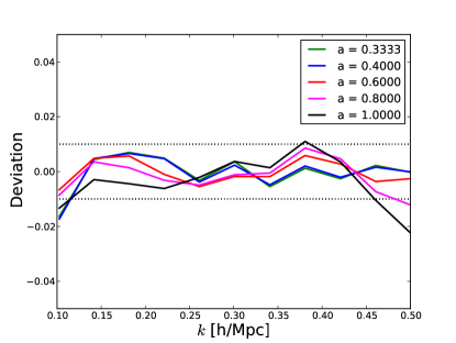
Figure 9 shows that using Eq. (36) the accuracy in reconstructing the nonlinear, real space matter power spectrum is $\sim$1% over the range $k=0.12-0.46\,h$/Mpc. By comparison, Halofit for $\Lambda$CDM is accurate to 5-10% over this same range Heitmann:2008eq , with the revised Halofit of 12082701 good to 5%. Moreover, the analytic form of Eq. (36) is extremely simple. We emphasize that so far this has only been tested for the M000 cosmology. In the next stage of our work, when we use the other Coyote simulations to explore cosmology dependence, it will be interesting to see if the form holds and how the parameters depend on cosmology.

Figure 9: Fractional difference between the nonlinear, real space power spectrum measured on M000 and the analytic RealEasy form is plotted vs wavenumber. Curves are for $a=0.33$, 0.4, 0.6, 0.8, 1, from top to bottom at $k=0.5\,h$/Mpc.

References

- (1) Baryon Oscillation Spectroscopic Survey: D.J. Eisenstein et al, Astron. J. 142, 72 (2011) [arXiv:1101.1529] ; http://www.sdss3.org/surveys/boss.php
- (2) Dark Energy Spectroscopic Instrument: D. Schlegel et al, arXiv:1106.1706 ; http://desi2013.lbl.gov
- (3) Prime Focus Spectrograph: R. Ellis et al, arXiv:1206.0737 ; http://sumire.ipmu.jp/en/2652
- (4) N. Kaiser, MNRAS 227, 1 (1987)
- (5) T. Matsubara, A.S. Szalay, Phys. Rev. Lett. 90, 012302 (2003) [arXiv:astro-ph/0208087]
- (6) R. Scoccimarro, Phys. Rev. D 70, 083007 (2004) [arXiv:astro-ph/0407214
- (7) A. Taruya, T. Nishimichi, S. Saito, Phys. Rev. D 82, 063522 (2010) [arXiv:1006.0699]
- (8) J. Tang, I. Kayo, M. Takada, MNRAS 416, 2291 (2011) [arXiv:1103.3614]
- (9) B.A. Reid, M. White, MNRAS 417, 1913 (2011) [arXiv:1105.4165]
- (10) E. Jennings, C.M. Baugh, S. Pascoli, Mon. Not. Royal Astron. Soc. 410, 2081 (2010) [arXiv:1003.4282]
- (11) J. Kwan, G.F. Lewis, E.V. Linder, ApJ 748, 78 (2012) [arXiv:1105.1194]
- (12) U. Seljak, P. McDonald, JCAP 1111, 039 (2011) [arXiv:1109.1888]
- (13) J. Kwan, Ph.D. thesis, University of Sydney (2011)
- (14) T. Okumura, U. Seljak, P. McDonald, V. Desjacques, JCAP 1202, 010 (2012) [arXiv:1109.1609]
- (15) T. Okumura, U. Seljak, V. Desjacques, JCAP 1211, 014 (2012) [arXiv:1206.4070]
- (16) Z. Vlah, U. Seljak, P. McDonald, T. Okumura, T. Baldauf, JCAP 1211, 009 (2012) [arXiv:1207.0839]
- (17) E.V. Linder, J. Samsing, JCAP 1302, 024 (2013) [arXiv:1211.2272]
- (18) K. Heitmann, M. White, C. Wagner, S. Habib and D. Higdon, Astrophys. J. 715, 104 (2010) [arXiv:0812.1052 [astro-ph]].
- (19) K. Heitmann, D. Higdon, M. White, S. Habib, B. J. Williams and C. Wagner, Astrophys. J. 705, 156 (2009) [arXiv:0902.0429 [astro-ph.CO]].
- (20) E. Lawrence, K. Heitmann, M. White, D. Higdon, C. Wagner, S. Habib and B. Williams, Astrophys. J. 713, 1322 (2010) [arXiv:0912.4490 [astro-ph.CO]].
- (21) R.E. Smith et al, MNRAS 341, 1311 (2003) [arXiv:astro-ph/0207664]
- (22) R. Takahashi, M. Sato, T. Nishimichi, A. Taruya, M. Oguri, ApJ 761, 152 (2012) [arXiv:1208.2701]