A Mass-Dependent Yield Origin of Neutron-Capture Element Abundance Distributions in Ultra-Faint Dwarfs

Abstract

One way to constrain the nature of the high-redshift progenitors of the Milky Way is to look at the low-metallicity stellar populations of the different Galactic components today. For example, high-resolution spectroscopy of very metal poor (VMP) stars demonstrates remarkable agreement between the distribution of [Ti/Fe] in the stellar populations of the Milky Way halo (MW) and ultra-faint dwarf (UFD) galaxies. In contrast, for the neutron capture (nc) abundance ratio distributions [(Sr, Ba)/Fe], the peak of the small UFD sample (6 stars) exhibits a significant under-abundance relative to the VMP stars in the larger MW halo sample ($\sim$ 300 stars). We present a simple scenario that can simultaneously explain these similarities and differences by assuming: (i) that the MW VMP stars were predominately enriched by a prior generation of stars which possessed a higher total mass than the prior generation of stars that enriched the UFD VMP stars; and (ii) a much stronger mass-dependent yield (MDY) for nc-elements than for the (known) MDY for Ti. Simple statistical tests demonstrate that conditions (i) and (ii) are consistent with the observed abundance distributions, albeit without strong constraints on model parameters. A comparison of the broad constraints for these nc-MDY with those derived in the literature seems to rule out Ba production from low-mass SNs and affirms models that primarily generate yields from high-mass SN. Our scenario can be confirmed by a relatively modest (factor of $\sim 3-4$) increase in the number of high-resolution spectra of VMP stars in UFDs.

1. Introduction

Our understanding of galaxies forming in a hierarchical universe suggests that a large fraction – and possibly the majority – of stars now in the halo of the Milky Way (MW) originally formed in smaller separate systems that were subsequently accreted and disrupted by our Galaxy (as originally proposed by Searle & Zinn, 1978), with the remainder formed in situ within the main Galactic progenitor (Eggen et al., 1962; Abadi et al., 2003a, b; Zolotov et al., 2010; McCarthy et al., 2012; Tissera et al., 2012). While the relative contributions of accreted and in situ populations remain uncertain, simulations in which the stellar halo is assumed to be formed entirely by accretion (Bullock & Johnston, 2005; Cooper et al., 2010) have been shown to have levels of substructure in space, velocities and stellar populations that are broadly consistent with observations (Bell et al., 2008; Schlaufman et al., 2009; Xue et al., 2011). This raises the following question: to what extent can the small systems that survive today (e.g. the satellite galaxies of the MW) be exploited to understand the properties of the small systems that fell in long ago (i.e. the primordial progenitors of the MW halo)?

One approach to this question is to compare and contrast the chemical abundance patterns of the stars in the stellar halo with those in satellite galaxies. For example, at metallicities [Fe/H] $\gtrsim-2$, stars in the low-mass classical dwarf spheroidals generally have lower $\alpha$-element abundances than halo stars (as seen in compilations by Venn et al., 2004; Geisler et al., 2007). The observed differences can be explained, in general, by the low star formation rates and efficiencies detected in low mass dwarf spheroidals versus the likely progenitors of most halo stars (see, e.g., review by Tolstoy et al., 2009). Assuming a continuous star formation history, it is true that for all galaxies there exists an epoch for which no appreciable contributions from Type Ia supernovas (which predominantly produce the decline in [$\alpha$/Fe]) are seen. This means that cosmological and astrophysical effects, which can prematurely quench star formation in galaxies such as reionization (Hoeft et al., 2006) and ram pressure stripping (Mayer et al., 2006), may determine whether low $\alpha$-abundance ratios appear in systems that are accreted early-on. Therefore, these differences can also be explained within the hierarchical picture of structure formation as a result of star formation histories of the surviving satellites being much more extended than those of the progenitors of the bulk of the Halo (Robertson et al., 2005; Font et al., 2006). However, this statement pertaining to late-time evolution still begs the question: to what extent are the progenitors of the stellar halo similar to the progenitors of the MW’s satellite galaxies? This can be addressed by comparing the abundance patterns of stars found in the “Very Metal Poor” (VMP) tail of the metallicity distribution (specifically those VMP stars with [Fe/H] $<-2.5$) which, because of their low metallicities, are supposed to have formed early on in the history of the Universe.

Figure 1.— A compilation of data reproduced from (Frebel, 2010) showing a comparison in abundance ratio patterns with Fe for Ti and two nc-elements (Sr, Ba) versus [Fe/H]. Top: Distribution of [Ti/Fe] in MW halo stars (black open triangles) versus UF stars (green upside-down triangles). Middle: Distributions for [Sr/Fe] (nc-element abundance ratio). Bottom: Distributions for [Ba/Fe] (nc-element abundance ratio). Adjacent panels on the right show the relative number distributions, binned by 0.2 dex, for all stars below [Fe/H] = -2.5. Note that stars with upper limits are not included here. See §4.2 for details.

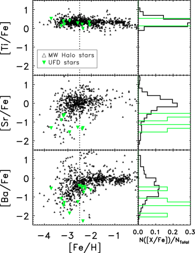
The open black triangles in the top panel of Figure 1 demonstrate that the stellar halo has an average Titanium-to-Iron abundance ratio ([Ti/Fe]) that is roughly constant at all metallicities (measured by [Fe/H]), with a small dispersion that widens in the VMP population. This dispersion can arise when the stochastic nature of star formation is convolved with chemical yields that depend on the masses of the enriching stars (Audouze & Silk, 1995; Ryan et al., 1996; McWilliam, 1997, 1998; Norris et al., 2000). For example, Karlsson & Gustafsson (2005) point out that some VMP stars inherit their chemical compositions from gas enriched by just one or a few supernovae (SNe) and have the potential to reflect the full range of abundance ratios implied by the yields from stars of different masses (see also the discussion in Karlsson, 2005; Tumlinson, 2006; Carigi & Hernandez, 2008; Koch, 2009; Bland-Hawthorn et al., 2010). Indeed, the range in [Ti/Fe] exhibited in the stellar halo data at low [Fe/H] is consistent with the predictions for the range in individual yields of Ti from models of exploding stars of different masses (Nomoto et al., 2006; Heger & Woosley, 2010). In contrast, most stars found with higher metallicities must have been enriched by many SNe, so all their abundances are closer to the average yield for the combined population which can be estimated by integrating the mass-dependent yields (MDY) of the individual stars over the initial mass function (IMF) of enriching stars.

The black open triangles in the lower panels of Figure 1 reveal a much wider spread in abundance ratios for the neutron-capture (nc) elements (here, Barium (Ba) and Strontium (Sr)) for VMP stars found in the stellar halo compared to Ti in the upper panel. At these metallicities, Roederer et al. (2010) suggest (see their Figure 13) that the same massive stars that produce Ti (and the $\alpha$-elements it emulates) also produce nc-elements (thought to originate from core-collapse SN explosions via the r-process and perhaps from AGB/pre-SN winds via the s-process) but the forms of the MDYs for Sr and Ba are essentially unknown. Hence, one viable explanation of the observed difference in the abundance ratio range between Ti and nc-elements for VMP stars is to again appeal to the stochastic nature of metal enrichment, but now assume a much stronger MDY for nc-elements than for Ti.

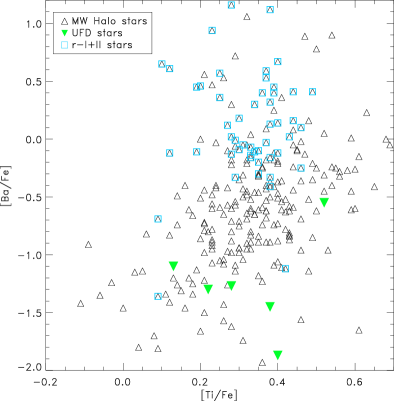
The green upside-down triangles in Figure 1 show abundance ratio measurements in stars in the ultra-faint dwarf satellites (UFD) of the MW (Frebel et al., 2010; Norris et al., 2010; Simon et al., 2010; Frebel, 2010, and references therein). The Ti distributions for the VMP stars in the UFDs (green upside-down triangles) are very similar to the stellar halo (black open triangles), while the nc distributions show a significant difference, with a clear offset between the medians of the two populations that exceeds the spread due to systematic and observational errors (Frebel, 2010). Several types of “differences” can be invoked to explain the origin of the galaxy-dependence of these abundance ratio distributions:

1. Differences in the mixing of Ti versus nc-elements due to differences in the formation site and process for each element, and, as a consequence, differences in the resultant properties of the enriched ejecta. Assuming that MW progenitors are predominantly larger in size, gas content, and dark matter mass than UFD progenitors, the strength of this effect is mediated by two environmental factors: (i) the depth of the gravitational potential dictates to what extent the different products can be blown out of their respective galaxies by core-collapse SNe; and (ii) the size and dynamics of local gas reservoirs influences how far the products can be evenly mixed in their respective galaxies.

2. Differences in the IMF or MDY of enriching stars due to preferential enrichment of UFDs from primordial populations of hypernovae (Nomoto et al., 2006) and/or pair-instability SN (PISN) ejecta from Pop III stars (see Frebel & Bromm, 2012, and their “Case B” for a discussion of these scenarios).

3. Differences in the total masses of stars enriching the VMP populations in the MW halo and UFD (hereafter the “stochastic argument,” similar to Case A of Frebel & Bromm, 2012).

Note that all of the explanations above implicitly assume that the UFD progenitors are chemically isolated from MW halo progenitors, which has recently been demonstrated to be a plausible supposition in an analysis of N-body simulations by Corlies et al. (2013).

In this paper, we restrict our attention to the last of these “differences”, which we consider the simplest model possible. We extend the discussion of dispersions and skews already in the literature to look at how stochastic chemical enrichment can influence the full shape of chemical abundance ratio distributions. Our aim is to isolate the influence of this one effect alone. Specifically, we examine to what extent the current abundance ratio distributions of VMP stars in the MW halo and UFDs can be explained without appealing to differences in mixing, varying the IMF or adopting unique yields. In §2, we outline and describe the assumptions made in our models. In §3, we present the general trends in the shapes of abundance ratio distributions produced by our models due to stochastic enrichment. In §4, we determine the likelihood of drawing the observed distributions of abundance ratios (found in the MW halo and the UFDs) from our simple models. In §5, we discuss the implications and limitations of our results in connection with expectations from other related studies. Finally, in §6, we summarize our results and discuss a possible test of the scenario with near-future observations.

2. General Approach

Our aim is to determine whether a simple model can simultaneously explain both the similarities in the distribution of [Ti/Fe] and the differences between the distributions of [(Sr,Ba)/Fe] seen for the two systems (the MW halo and the UFDs) represented in Figure 1. In our model, we assume that: i) the abundance ratios in each observed star represents enrichment from a previous enriching stellar generation (ESG); (ii) the stars within each ESG are sampled from a “normal” (Salpeter) IMF and produce enrichment with a power-law MDY; and iii) the stellar abundance ratio distributions for each system are the signature of enrichment from an ensemble of ESGs of a characteristic mass, M_ESG. Note that our simple model assumes that enrichment from Pop III, metal-free stars with peculiar yields does not have a significant effect on abundance ratio patterns at the metallicities observed in UFDs.

2.1. Enriching stellar generation

Each ESG represents the combined enrichment by stars of total mass $M_{\rm ESG}$ that could be formed in one or many different star clusters. Each ESG realization results from a Monte-Carlo sampling of a Salpeter (1955) IMF where

$$\xi=\frac{dN}{dm}=m^{-\alpha}$$ (1)

and $\alpha=2.35$. We assume that the lower and upper stellar mass limit for the IMF are $m_{\rm low}=0.08M_{\odot}$ and $m_{\rm upp}=40$, respectively. (In Appendix A, a range of upper stellar mass limits, $m_{\rm upp}=30-80M_{\odot}$, are explored.) The lower threshold for stars contributing to chemical enrichment is taken to be $m_{\rm enrich,low}=8M_{\odot}$. The number of draws from the IMF is determined by the total and, subsequently, the remaining mass available to form a ESG of $\sim M_{\rm ESG}$. Since this sequence of draws terminates when the total mass drawn exceeds $M_{\rm ESG}$, the actual ESG created only approximates the designated mass.

2.2. Stellar enrichment

Each ESG realization produces a total mass yield for each element $X$ by summation over all individual yields $m_{X}$ generated from stars of masses $m\geq 8M_{\odot}$. These yields are determined by a power law of index $\kappa_{X}$ and normalization $\beta_{X}$:

$$m_{\rm X}=\beta_{\rm X}\cdot m^{\kappa_{\rm X}}$$ (2)

In our models, we are assuming that the sources of enrichment are the same in both UFD and MW halo stars.

Currently, our models only take into account stellar enrichment from massive, short-lived stars which are thought to be the dominant source of enrichment for the VMP populations in both systems. Enrichment by long-lived, low mass stars (excluding binaries) is assumed to become important only at higher metallicities. Although Ba is an archetypical s-process element at higher metallicities, the trace amounts of Ba observed in the VMP stars we are modeling are produced in core-collapse SNe by the r-process. There is also a large number of stars with measurable Sr abundances for the same VMP population even though Sr is primarily an s-process element thought to originate from the AGB phase in low-mass stars (known as the main s-process). Therefore, we anticipate that Sr-enrichment in the VMP population comes from a short-lived, but intense, pre-SN/super-AGB phase from massive stars, contributing weak s-process elements to the ISM prior to the SN phase (Herwig, 2005); or, perhaps, is simply indicative of r-process at low metallicities (Roederer et al., 2010). Recent evidence pointing to fast rotating, massive stars as a viable source for s-process elements like Sr can be found in Chiappini et al. (2011), Frischknecht et al. (2012), and references therein. Hence, $m_{X}$ in our models represents a combined effective yield from both the pre-SN and SN phases of a star of mass m$\geq 8M_{\odot}$.

To construct abundance ratios, we first need to account for the common denominator — Fe abundance. The theoretical yield for Fe tabulated in Nomoto et al. (2006) varies only slightly over the range of enriching stellar masses examined — indeed, some previous studies using theoretical Fe yields of $\gtrsim 0.05M_{\odot}$ have assumed invariant Fe yields for SN ejecta. For consistency with other yields adopted in our models, we set yield parameters for Fe by fitting a power law to the Nomoto et al. (2006) predictions to find $\beta_{\rm Fe}=$ 0.0607 $M_{\odot}$ and $\kappa_{\rm Fe}=0.072$.

Figure 2.— Left: Log-log plot of element mass yield versus progenitor stellar mass showing linear fits (black solid lines) with parameters $\beta_{X}$ and $\kappa_{X}$ for some $\alpha$-elements, Ti and Fe MDYs from Nomoto et al. (2006). Right: Linear plot of element mass yield versus progenitor stellar mass showing the derived power-law fits (black solid lines) for each element shown in the left plot.

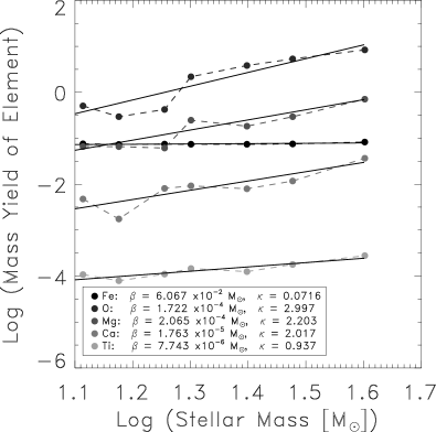
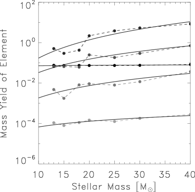
Figure 2 shows our fits to the Nomoto et al. (2006) theoretical yields at Z = 0.001 ($\simeq Z_{\odot}/18$) for Fe along with fits to archetypical $\alpha$-element MDYs. Also shown is our fit for Ti, which we chose as our known theoretical MDY because it exhibits the lowest scatter around a power-law fit and has a weak MDY.

For Ti, the power law fit yields an index of $\kappa_{Ti}=0.937$. The yield normalization $\beta_{Ti}$ is adjusted to maintain agreement between the average abundance ratio calculated for our assumed IMF, $\left<\left[\frac{\rm Ti}{\rm Fe}\right]\right>_{\rm IMF}(\beta_{Ti},\kappa_{Ti})$, and average observed abundance ratio, $\left<\left[\frac{\rm Ti}{\rm Fe}\right]\right>_{\rm OBS}$, calculated for our VMP ([Fe/H] $<$ -2.5) MW halo sample (see Appendix B). This adjustment is made to compensate for the failure of the Nomoto models to get the amount of “fallback” for Ti correct in their SN explosions (for an explanation, see Figure 12 and §8.2 in their paper).

For Sr and Ba, which have no firm yield predictions, we examine a range in $\kappa_{X}$ ($-20\leq\kappa_{X}\leq 20$) which is wide enough to reveal the relative effects of stochastic sampling in ESGs of different mass (see §4.3-4.4) and allows for a comparison to some proposed yields in the literature (see §5.1). For each $\kappa_{X}$ a $\beta_{X}$ is derived by again requiring a match to the observed average in the MW halo sample, assumed to arise from the fully-sampled IMF.

Finally, it should be noted that while we do track the production of Fe in each ESG realization, we do not explicitly follow evolution in [Fe/H] since the latter is not critical to the scope of this project and would require more detailed assumptions regarding star formation efficiency, mixing, infall, and blowout.

2.3. Parent distributions and synthetic “Child” samples

Following the prescription given in §2.2, each ESG realization from §2.1 produces a chemical abundance ratio for [X/Fe] (where $X$ represents Ti, Ba or Sr), which is supposed to represent a possible enrichment pattern for a subset of the total population of stars that exist in the observed systems. Thus, each ESG produces one enrichment pattern from which many stars can sample. However, the numbers are proportional to how common that enrichment pattern is (as determined by the distribution of patterns from the ESGs generated). For a given set of parameters ($M_{\rm ESG}$, $\kappa_{\rm X}$) we construct two-dimensional “parent distributions” in the [Sr/Fe]-[Ti/Fe] and [Ba/Fe]-[Ti/Fe] planes from ensembles of enrichment by 1000 ESGs. Each parent represents a model for the intrinsic stellar distribution from which we can draw random synthetic samples (“children”) to compare to the MW halo and UFD observed data distributions. Each child contains the same number of synthetic stars as the number of observed stars and their stellar abundance ratios are scattered by observational errors which are taken to be 0.15 dex (as a conservative lower bound).

3. Results I: General Effects

In this section we develop some intuition by examining the effect of varying parameters ($M_{\rm ESG}$, $\kappa_{\rm X}$) on the shape of the abundance ratio distribution in [$X$/Fe] in one dimension.

3.1. Phenomenological expectations

Figure 3 illustrates schematically the trends we expect to see in our distributions resulting from the combination of the IMF, the MDY($\kappa_{\rm X}$), and the number of enriching stars, n_⋆, generated in a ESG (which is proportional, on average, to $M_{\rm ESG}$).

Figure 3.— A schematic displaying the assumptions of our model and the various effects that arise from convolving the IMF, MDY, and the number of enriching stars per ESG, n_⋆, together. Note that n_⋆ is not exactly proportional to the characteristic ESG mass, $M_{\rm ESG}$, due to stochastic sampling of the IMF. However, n_⋆ does give some indication of the magnitude of $M_{\rm ESG}$. Panel A shows a plot of the Salpeter IMF used in our models, indicating a large ratio of low-to-high mass stars produced in ESGs. Panel B displays three different MDY “strengths” measured by the slope $\kappa_{\rm X}$ as indicated by approximately zero (dotted), low (dashed), and high (solid) labelled lines. These MDY strengths result in the trends we expect to find in abundance ratio distributions for VMP stars (shown in panel C). Panel C shows the three types of distributions that can arise for different positive MDYs resulting from the convolution of the IMF and MDYs for four different characteristic values of n_⋆. The shades/outlines of the distributions represent the “strength” of the MDY (as shown in panel B): $\kappa\sim 0$ (dark grey; dotted line), $\kappa\sim$ low (grey; dashed line), and $\kappa\sim$ high (light grey; solid line).

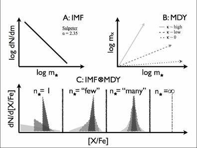
In panel A, the Salpeter IMF is shown, illustrating that many more lower mass stars are produced for a given number of high mass stars in any ESG. This property is generic to all proposed IMFs in nearby galactic environments investigated in the literature (Kroupa, 2002; Chabrier, 2003; Elmegreen & Scalo, 2005; Elmegreen, 2006, 2007).

In panel B, the MDY for various $\kappa_{\rm X}$ are shown: an approximately constant mass yield across all stellar masses ($\kappa_{\rm X}\simeq 0$), a small/weak change in mass yield (low $\kappa_{\rm X}$ values), and a large/strong change in mass yield (high $\kappa_{\rm X}$ values). It should be noted that these power law fits are a rough 1^st-order approximation to the non-monotonic functions for MDYs anticipated in nucleosynthetic yield models (e.g. Nomoto et al., 2006; Heger & Woosley, 2010) for both Ti and nc-elements. The detailed shape of these functions will be another key factor which contributes to the range and shape of observed abundance ratios, but is not considered in this paper to keep our models as simple as possible (and because the mass-dependence of stellar yields for most elements is not well understood at present).

In panel C, trends in the distribution of yields from an ensemble of enriching ESGs as a result of combining the IMF with MDY (IMF$\otimes$MDY) are shown for different numbers of enriching stars per ESG, n_⋆.

In the limit of n_⋆= $\infty$ (right hand plot of panel C) complete sampling of the IMF is achieved, resulting in a single mean value

$$\left<\left[\frac{\rm X}{\rm Fe}\right]\right>_{\rm IMF}=\left<\left[\frac{\rm X}{\rm Fe}\right]\right>_{\rm OBS}$$ (3)

for all realizations.

In the opposite limit of n_⋆=1 (left-hand plot of panel C), we expect to directly sample the full range of yields contributed from individual stars, with frequencies dictated by the IMF. Hence a strong MDY (high $\kappa_{\rm X}$; solid line/light-shaded area) will produce a wide distribution while a weak MDY (low $\kappa_{\rm X}$; dotted line/dark-shaded area) will produce a narrow one. For positive $\kappa_{\rm X}$, the skew of these distributions will be positive or right-skewed, meaning that their extended tails are found to the right of the median and peaks are found to the left. In the case of negative $\kappa_{\rm X}$ (not shown), the skew of the distributions will become negative, with the extended tail to the left of the median. A wide range of distributions can be observed between these two limits. For an element X with large, positive $\kappa_{\rm X}$ (solid lines and light-gray areas in Figure 3), various distributions can be exhibited depending on the value of n_⋆.

For example, with n_⋆=“few”, the convolution of yields with the IMF from a few enrichers can generate negatively-skewed (left-skewed) distributions. Although massive enrichers are found less frequently than their lower mass counterparts, their individual chemical yields can dwarf those contributed by lower mass stars. Hence, the orientation of the tail of the distribution can flip compared to the $n_{\star}=1$ case due to the weighted contribution of the “few” high mass enrichers with large absolute yields.

For n_⋆=“many”, the average number of n_⋆ realized in each ESG is high enough to start altering the distribution from a poisson-like distribution to a gaussian-like distribution via the law of large numbers. This effect arises from a counter-balance between the plentiful, although low impact, low-mass enrichers and the sparse, yet high impact, high-mass enrichers which leads to an “erosion” of possible abundance ratios at the margins of the distribution (homogenization), thus narrowing the distribution in accordance with the central limit theorem.

3.2. Model distributions

We can assess the validity of our phenomenological expectations, given in §3.1, by examining ensembles of many ESGs realized with identical parameters, to create chemical abundance ratio probability distributions. The features of interest are systematic changes in the: 1) variance (dispersion), 2) skewness (lopsidedness), and 3) kurtosis (peakedness) of the distribution. As noted in §2.2, the “means” of our distributions are set by the observed average abundance ratio but these higher moments emerge from the parameters specified for $\kappa_{\rm X}$ and $M_{\rm ESG}$.

Figure 4.— Distributions of abundance ratios produced from 1000 realizations of an ESG, with $M_{\rm ESG}=10^{2}M_{\odot}$ (left panel), $10^{3}M_{\odot}$ (middle panel), and $10^{4}M_{\odot}$ (right panel). Color of the distribution refers to the corresponding $\kappa_{X}$ used for the MDY: 3 (red), 6 (green) and 9 (blue). The black vertical dotted line shows the average for all ESGs with $\kappa_{X}$ = 0. The average number of enriching core-collapse supernovas are represented by $<$$n_{\star}$$>$.

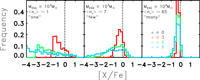
Figures 4 and 5 illustrate the general trends found for various parameters ($\kappa_{\rm X}$, $M_{\rm ESG}$). Figure 4 shows a number of features in these distributions that are similar to both our schematic framework and the observed distributions. Each panel corresponds to a different decade in $M_{\rm ESG}$ ($=10^{2},10^{3},10^{4}M_{\odot}$ respectively) realized 1000 times to create distributions with average number of enriching stars given by $<$$n_{\star}$$>$ $\simeq 1$, $\simeq 7$, and $\simeq 65$, analogous to the one, “few”, and “many” enrichers in the schematic in Figure 3. Comparing the different colored histograms within each panel, increasing the value of $\kappa_{X}$ = 3 (red), 6 (green) and 9 (blue) leads to a broadening of the distribution. The black vertical dotted line shows the average for the distributions which correspond to yields from all ESGs generated with $\kappa_{X}$ = 0. Comparing the same colored histograms across the panels, shows stochastic effects producing right-skewed distributions for $n_{\star}\sim 1$ (left panel), left-skewed distributions for $n_{\star}\sim$ “few” (middle panel) and gaussian-like distributions for $n_{\star}\sim$ “many” (right panel).

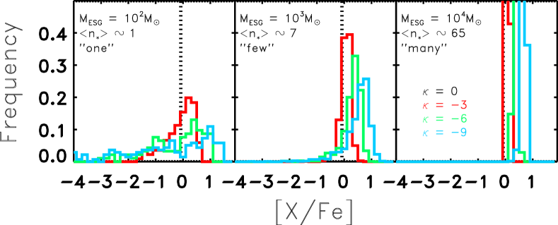
Figure 5 shows the general trends for negative MDYs. A comparison between Figure 4 and Figure 5 demonstrates that distributions derived with positive MDYs for X cause negatively or positively skewed distributions while negative MDYs only lead to negatively skewed distributions.

Most importantly, if we compare Figure 4 to the observations (“by eye”) we see that the simple stochastic picture can be supported if the following criteria are met:

• Abundance ratios in MW halo stars reflect enrichment by ESG with masses sufficient to produce “few”-to-“many” enrichers, while abundance ratios in UFD stars reflect enrichment by ESG with masses that would produce roughly “one” enricher;

• Ti is well approximated by low $\kappa_{\rm X}$, resulting in a similar distribution for any $n_{\star}$ (or $M_{\rm ESG}$);

• nc-element yields are well approximated by high $|\kappa_{\rm X}|$, resulting in noticeably different distributions for low versus high $n_{\star}$ (or $M_{\rm ESG}$).

Figure 5.— Figure is the similar to Figure 4 but shows distributions derived from negative MDYs.

4. Results II: Observational Constraints On Model Parameters

Having demonstrated in principle that skewed abundance ratio distributions can be obtained when incomplete sampling of the IMF is coupled with strong MDYs we now assess whether this explanation is sufficient to explain the current observed samples.

4.1. Selecting a comparison sample

As stated earlier, our models were designed to track stellar abundance ratios that originate from the evolution of high-mass stars that are not in binary systems (i.e., the combined yields from a super-AGB/pre-SN phase and/or post-SN wind). Hence we select our sample from the Frebel (2010) compilation to exclude stars whose abundance ratios are likely to include enrichment from other sources.

Specifically, abundance ratio contributions from low-mass stars (e.g. AGB winds or Type Ia SNe) are limited by looking at VMP stars (with [Fe/H] $<$ -2.5 in our case): because of their low-metallicity, VMP stars are assumed to have formed before long-lived low-mass stars had a chance to contribute significantly to chemical enrichment Vargas et al. (2013).

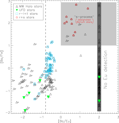
In addition, we use Figure 6 to exclude stars whose abundance patterns could reflect enrichment during binary evolution by identifying those stars that fall within the abundance ratio boundaries of [Ba/Fe] $>1.0$ dex and [Ba/Eu] $>0.5$ dex (indicated by the grey rectangular region, from the diagnostic prescription listed in the review by Beers & Christlieb, 2005). These “Barium stars” are thought to be produced during binary evolution from s-process-enhanced Barium enrichment in the common envelope (Smith & Lambert, 1990; McClure & Woodsworth, 1990) or wind accretion (Boffin & Jorissen, 1988) phases. The validity of this simple diagnostic is confirmed by the locations of the stars highlighted in red and blue which indicate where Frebel (2010), using a more detailed abundance ratio analysis, designated stars as enriched by both r+s-process (in red) or by r-process (either class I or II) alone (in blue). For those stars with no Eu detection (vertical grey stripe) we also exclude those stars with [Ba/Fe] $>$ 1.0 dex since a non-detection for Eu ensures that [Ba/Eu] $>>0.5$ dex.

Figure 6.— [Ba/Fe] vs. [Ba/Eu] for the VMP (below [Fe/H] = -2.5) stars in the MW halo/UFD data set. Black triangles are MW halo stars without given r- or s-process abundance ratio designations. Blue squares refer to stars with r-process abundance ratios (either class I or II) and red diamonds refer to r+s-process stars as designated by Frebel (2010). The pure r-process upper-limit, designated Barium stars (exclusion) region, and stars with non-detections of Europium and identified by a dashed grey line, grey rectangular region, and dark grey stripe, respectively (see text for explanation).

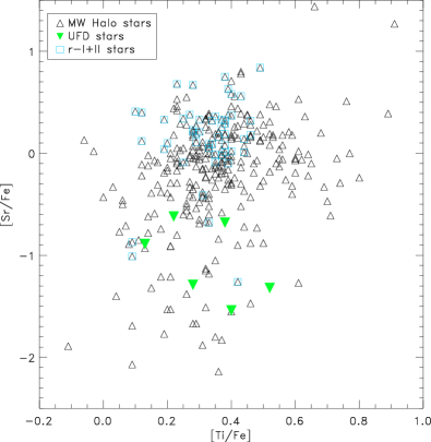
Figures 7 and 8 display our final samples in the [Sr/Fe]-[Ti/Fe] and [Ba/Fe]-[Ti/Fe] planes containing 322 stars ($n_{\rm MW}=316$ and $n_{\rm UF}=6$) and 269 stars ($n_{\rm MW}=263$ and $n_{\rm UF}=6$), respectively. As noted above, these samples are limited to stars not designated as “Barium stars” with [Fe/H] $<-2.5$. In addition, only stars with values for both elements (either Sr and Ti or Ba and Ti) that are definitively measured are included (i.e. excluding upper limits).

Figure 7.— [Sr/Fe] vs. [Ti/Fe] for our compiled observed MW halo/UFD data set. Symbols are the same as those defined in Figure 6.

Figure 8.— [Ba/Fe] vs. [Ti/Fe] for our compiled observed MW halo/UFD data set. Symbols are the same as those defined in Figure 6.

4.2. Comparing data and models with a “paternal likelihood test”

To directly compare our models to observations, we construct a test to determine the likelihood that the observed stellar abundance ratio samples for the MW halo or UFDs, shown in Figures 7 and 8, could be drawn from the 2-d parent distributions generated by a particular parameter set (see §2.3). Our “paternal-likelihood test,” is built around the comparison of our samples to each parent using the D-statistic derived from the two-dimensional Kolmogorov-Smirnov (2dKS) test (Press, 1992). The D-statistic represents the maximum difference (supremum) between two cumulative distribution functions (CDFs) — a smaller supremum indicates a higher likelihood that both CDFs are drawn from the same population.

While the values of the D-statistic can be used to rank our parameter sets given the observed data, the 2dKS test alone is insufficient for our purposes. The multitude of possible data orderings used to create CDFs in multi-dimensional samples (Peacock, 1983; Fasano & Franceschini, 1987) means that the D-statistic cannot be simply converted to a likelihood in a model-independent manner. This problem is particularly challenging given the small number of stars (6) used in the UFD samples where large differences in D-statistics between parameter sets may not actually represent significantly different likelihoods. Our paternal-likelihood test addresses this limitation by generating child-parent distances (${\rm{\it D}_{\rm cp}}$) for a large number of synthetic child samples (with sample sizes equaling the observed data size) drawn (bootstrapped) from the parent. The distribution of ${\rm{\it D}_{\rm cp}}$ can then be used to assess the likelihood of observing the distance ${\rm{\it D}_{\rm dp}}$ between the collected data samples and the parent.

Specifically, we generate $n_{\rm children}=100$ from each parent (defined by parameters $M_{ESG}$, $\kappa_{\rm X}$, $m_{\rm upp}$). Each child is comprised of n randomly-sampled stellar abundance ratios from the parent distribution where n equals the number of observed stars from the observed comparison data sample. Figure 9, for example, shows a distribution of D-statistic ranks calculated for the [Ti/Fe]-[Ba/Fe]-plane using children drawn from one of our parent distributions to assess parental likelihood for the MW halo (upper panel) and UFDs (lower panel), respectively. The spreads in the distributions are influenced by both the observational/systematic errors and the sample size. As expected, a larger sample of stellar abundance ratios increases our certainty about the likely parent of the observed distribution.

We assess the significance of the comparison rankings between the observational data and the parent, $D_{\rm dp}$ (indicated by vertical dashed line in Figure 9) by calculating a p-value — i.e. the fraction of children that are ranked as more different from the parent than the observed data (shown as the fraction of the histogram that lies to the right of the vertical line in Figure 9):

$${\rm{\it p}-value}=\frac{n_{\rm children}({\rm{\it D}}_{\rm cp}>{\rm{\it D}}_{\rm dp})}{n_{\rm children}}.$$ (4)

The higher the p-value, the more likely the observed abundance ratios are a potential “offspring” of the parent.

Figure 9.— Histograms show the distributions of the child-parent D-statistic, $D_{\rm cp}$, for “children” with the same size as the observed Ba data sets ($n=316$ for MW, upper panel; $n=6$ for UFDs, lower panel) drawn from parents with model parameters $\kappa_{X}$ = 9.5, ${M_{ESG}}^{MW}$ = $10^{3.5}M_{\odot}$ (top) and ${M_{ESG}}^{UF}$ = $10^{2.0}M_{\odot}$ (bottom). Bin sizes equal $|$D_Max-D_Min$|/10$ in D range. The vertical line marks the D-statistic for the observed data sets, ${\rm{\it D}}_{\rm dp}$.

4.3. Results from the [Ti/Fe]-[Sr/Fe] plane

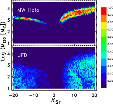
Figure 10 summarizes the results of our paternal likelihood test applied to the MW halo (upper panel) and UFD (lower panel) samples in the [Ti/Fe]-[Sr/Fe] plane. The color of the plot indicates the likelihood (i.e. the p-value) of the observations being drawn from a parent of particular $M_{\rm ESG}$ and $\kappa_{\rm X}$, and for a fixed $M_{\rm upp}=40M_{\odot}$.

From the upper panel it is immediately apparent that models with $M_{\rm ESG}\gtrsim 10^{3}M_{\odot}$ are preferred in generating MW halo-like distributions. Furthermore, these models are consistent with a wide range of $|\kappa_{\rm X}|\gtrsim 2$ values due to the degeneracy between stochastic sampling of the IMF (governed by $M_{\rm ESG}$) and the effect of varying the strength of the MDY: the IMF is more completely sampled as $M_{\rm ESG}$ gets larger which will tend to homogenize the stellar abundance ratios, but this effect can be compensated for with a higher MDY strength in order to maintain a sufficient width to match the MW halo distribution.

Differences between the location and width of the trends apparent in the upper panel for $\pm\kappa_{\rm Sr}$ can be attributed to the relative weighting of low/high-mass enrichers in each case. Since there are significantly more low-mass enrichers than high-mass enrichers generated for $M_{\rm ESG}\gtrsim$ a few hundred solar masses, homogenization is reached sooner for negative $\kappa_{\rm X}$ (i.e. at a lower ESG mass) than for ESGs with a positive $\kappa_{\rm X}$. Also, the smaller width of the probability distribution for $\kappa_{\rm X}<0$ reflects the diminished contributions of high mass stars because they are (in this scenario) both rare and have yields that are small relative to their less massive counterparts, thus shrinking the range of $M_{\rm ESG}$ capable of producing the observed MW halo distribution.

The lower panel displays the results of the same analysis for the six stars in the UFD sample. The two regions of significant likelihood are analogs to the negative and positive $\kappa_{\rm X}$ trends found for the MW halo, but the paucity of observed stars in the UFD sample means that a much broader set of models are compatible with the observed chemical distributions. Therefore, we see models with substantial likelihoods (p-values) across more than two decades in $M_{\rm ESG}$ for a variety of $\kappa_{\rm X}$ values. Despite the breadth of possible solutions found in each panel, they demonstrate (as a whole) that our simple model of stochastic enrichment is sufficient to explain the Ti and Sr abundance ratio distributions in the MW halo and UFDs simultaneously, provided that: (i) the UFD systems were enriched by a lower ESG mass than the progenitors to the MW halo stars; and (ii) Sr yields can be characterized by a power law with a relatively larger $|\kappa_{\rm X}|$ when compared to Ti yields.

Figure 10.— Figure shows the likelihood (p-value) distribution for the MW halo (upper panel) and UFDs (lower panel) derived from different models with $M_{\rm upp}=40M_{\odot}$ (reflecting the [Ti/Fe]-[Sr/Fe] plane) as a function of $M_{\rm ESG}$ and $\kappa_{\rm X}$ for Sr yields. See text for explanation of features.

4.4. Results from the [Ti/Fe]-[Ba/Fe] plane

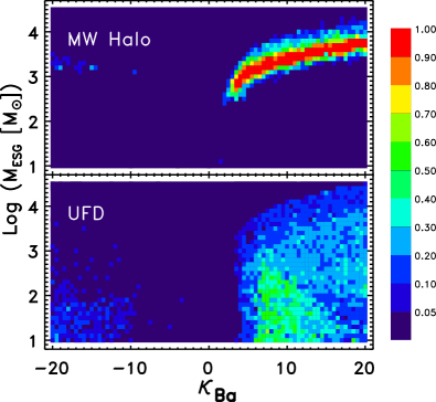
Figure 11 summarizes our analysis of model comparisons to samples observed in the [Ti/Fe]-[Ba/Fe] plane. This figure offers additional confirmation of the results from the [Ti/Fe]-[Sr/Fe] plane: that the same simple model of stochastic enrichment with the same masses for MW halo and UFD enrichers preferred can also explain the distributions in this plane. The UFD results here suggest a slightly lower $\kappa_{\rm X}$ for the MDY of Ba compared to Sr. Also, in the case of Ba, a negative MDY seems highly unlikely from our analysis. This result can be explained by comparing the UFD distributions from Figures 7 and 8 to the $M_{ESG}=10^{2}M_{\odot}$ models from Figure 5. It is apparent that a smaller negative offset along with a high concentration of abundances is favored in the models (Figure 5). A comparison of the observed distributions (Figures 7 and 8) reveals that [Sr/Fe] values are significantly more similar to the negative $\kappa_{\rm X}$ for $M_{ESG}=10^{2}M_{\odot}$ models than the [Ba/Fe] values. However, it should be noted that we rule out the existence of a negative $\kappa_{\rm Ba}$ based on the MW halo data as the current UFD data are inconclusive on their own. In the next section, our results for “allowed” MDY strengths are compared with the most recent yields found the literature.

Figure 11.— Figure is the same as Figure 10 for Ba yields.

Table 1Strength of Mass-Dependent Yields

Element	Metallicity	$\kappa_{\it empirical}^{8-10M_{\odot}}$ (r)a	$\kappa_{\textit{ab initio}}^{15-40M_{\odot}}$ (s)b	$\kappa_{\it inferred}^{15-40M_{\odot}}$ (s)c	This Work
(neutron-capture)	(Log Z)		(nr/rs)	(rs/ss)
	-5		$\sim$ 3.3/5.8	$\sim$ 6.5/6.7
Strontium (Sr)	-3	$\sim$ -15 or -18	$\sim$ 4.5/6.6	$\sim$ 7.4/—	$(\lesssim-10),(\gtrsim 7)$
	-5		—	$\sim$ 3.6/3.6
Barium (Ba)	-3	$\sim$ -15	—	$\sim$ 3.9/—	$\sim(6-12)$
a Derived from empirical yields given in Cescutti (2012).
b Derived from Figure 4.14 of Frischknecht (2012, PhD Thesis) for non-rotating (nr)/rotating stars (rs).
Yields for Ba were not given.
c Derived from Cescutti & Chiappini (2013) for rotating stars (rs) [their as-models]/spinstars (ss) [their
fs-models].
† Chieffi & Limongi (2004) and Limongi & Chieffi (2012) provide another set of theoretical MDYs for Sr.
From Chieffi & Limongi (2004) we find that the estimated MDYs for Sr given for progenitors with $z>0$
to $z\simeq z_{\odot}$ results in strengths that are $1\lesssim\kappa_{\rm Sr}\lesssim 4$. The MDY for Sr for zero metallicity stars is $\kappa_{\rm Sr}\simeq 8$
— compatible with our work. However, more recent work by the same authors (Limongi & Chieffi, 2012)
produces a $\kappa_{\rm Sr}\lesssim 5$ for zero metallicity stars. This result is only marginally compatible with our findings.

5. Discussion

In this section, we evaluate how our model-derived MDY strengths compare to others found in the literature. We also examine how our selection of data affects our reported results.

5.1. Comparison to Other MDY Estimates

In Table 1 we compare our derived MDY strengths to the latest predictions given in the literature. In particular, we compare our values to those extracted from ab initio yields (i.e. yields derived from simulations) for Sr given in Frischknecht (2012, PhD Thesis) and from inferred values from the ab initio- and empirically-derived yields (i.e. chosen to match observations) for Sr and Ba applied in Cescutti & Chiappini (2013).

• Empirical Yields for Sr and Ba ($8-10M_{\odot}$ production site) In Cescutti & Chiappini’s work, their homogenous stochastic models are chosen to fit the general distribution of halo stars without binary enrichment. These models, which they refer to as empirical models, are employed by the authors to examine the distributions produced by applying both their empirically-determined MDYs for the standard r- (and extended r-)process sites and the newly derived ab initio yields from Frischknecht’s thesis work. To generate MDY strengths for their empirical yields, we consult the figure of Sr and Ba yields given in Cescutti (2012) which are reported to be similar to the yields used in Cescutti & Chiappini (2013).

• ab initio Yields for Sr ($15-40M_{\odot}$ production site) In Frischknecht’s work, he conducts a suite of simulations that produce various chemical yields from massive stars as a function of the stars’ metallicity and rotation. From his work, we approximate ab initio strengths ($\kappa_{\textit{ab initio}}$) for ⁸⁸Sr by examining Figure 4.14 of Frischknecht (2012, PhD Thesis). Unfortunately, we are unable to make a direct comparison to MDYs strengths for Ba (which are also evaluated by Frischknecht) because they are not available in his published work.

• Inferred Yields for Sr and Ba ($15-40M_{\odot}$ production site) We also generate an estimate of the MDYs for Sr, and more importantly, for Ba (unreported) from Frischknecht’s unpublished results. To do this, we input the various inferred $\Delta[\frac{X}{Fe}]$, displayed in Figure 1 of Cescutti & Chiappini (2013), along with their progenitor stellar mass range into the difference between logarithmic values of Eqn. 2. If we assume that Fe-yields for these stars are weakly mass dependent, we get:

  $$\Delta\left[\frac{X}{Fe}\right]\sim Log\left(\frac{m_{X_{1}}}{m_{X_{2}}}\right)=\kappa_{X}\cdot Log\left(\frac{m_{1}}{m_{2}}\right)$$ (5)

  The estimates for the inferred MDYs strengths derived from Eqn. 5 are also listed in Table 1.

The final column of Table 1 gives our preferred MDY strengths, which are chosen by identifying ranges of $\kappa_{\rm X}$ that could be simultaneously compatible for BOTH the MW and UFD’s (i.e. looking at both upper and lower panels) As seen in Figure 10, both positive and negative MDY strengths for Sr are allowed. In particular, both a $\kappa_{\rm Sr}\gtrsim 7$, consistent with Frischknecht’s $15-40M_{\odot}$ ab initio yields and a $\kappa_{\rm Sr}\lesssim-14$, consistent with Cescutti’s $8-10M_{\odot}$ empirically-derived (standard r) yields, are favored for Sr. Additionally, the inferred $\kappa_{\rm Sr}$ from a combination of such yields should, in fact, be intrinsic to our analysis — however, inferences about combined yields are beyond the scope of this investigation and shall be addressed in future work.

Figure 11 shows us results for Ba yields. Positive MDYs with $\kappa_{\rm Ba}\sim 6-12$ are preferred and may be related to Frischknecht’s spinstar yields. However, the extremely low likelihoods for negative $\kappa_{\rm Ba}$ when compared to positive $\kappa_{\rm Ba}$, supports the notion that such yields are improbable. This strongly suggests a lack of Ba production from an $\sim 8-10M_{\odot}$ production site which is consistent with more recent hydrodynamic simulations (e.g., Fischer et al., 2010; Wanajo et al., 2011) but contrary to other expectations for nc-yields found in the literature (see, e.g., Cescutti & Chiappini, 2013; Cescutti, 2012; Qian & Wasserburg, 2008; Wanajo et al., 2003; Ishimaru & Wanajo, 1999; Wheeler et al., 1998; Mathews et al., 1992).

These preliminary results illustrate the advantage of using statistical techniques that address the full density of the observed distributions and not only the average of their spreads as implemented in Cescutti & Chiappini (2013) and other previous studies. Further development of this technique may provide the best chance to uncover the “galactic genealogy” of the MW and its closest companions in the Local Group.

5.2. Effects of Data Selection on Results

5.2.1 Data Compilations

One concern about using a compilation of data such as Frebel (2010) is that the dispersion in abundances may be artificially inflated by differences between the data sets. Frebel states that systematic difference between data sets are likely to inflate the dispersion by no more than 0.3 dex (for both the UFDs and MW halo). In particular, the dispersion between different measurements of Ti abundance (i.e., via Ti i/Ti ii or a combination thereof) is typically, $\sim$0.1–0.15 dex (e.g., Shetrone et al., 2003; Aoki et al., 2007; Frebel et al., 2010) which is precisely on par with observational errors. In contrast, both the offset (under-abundance) and scatter (dispersion) of nc-elements are a factor of $\sim$3–5 and $\sim$10 bigger than these systematic uncertainties, respectively. Thus, we conclude that the differences between surveys cannot significantly alter our current results. Moreover, artificially inflated dispersions for UFD and MW halo distributions would serve to decrease their expected M_ESG while leaving a significant $\Delta M_{ESG}$ between the distributions intact. Hence our result of lower M_ESG for UFDs verses significantly higher M_ESG for MW halo progenitors is insensitive to these systematic differences.

5.2.2 Ignoring Data with Upper Limits

Our parental likelihood test is not strictly applicable to samples containing upper limits. However, as a check, we apply the test to the Frebel data compilation, including upper limits, to determine the possible effects, if any, of leaving data with upper limits out of our analysis. Including the upper limits also increases the scatter of our MW halo samples, which, again, effectively decreases the inferred M_ESG slightly while, in this case, increasing the inferred MDYs. These values are not significantly different from the values we report. The similarity of the results from the two samples is compatible with the fact all stars with only upper limits for Sr and Ba are consistent with having [Sr/Fe] and [Ba/Fe] abundance ratios above those stars with the lowest known levels of nc-elements Roederer (2013); which is to say that stars with upper limits would actually be detected if higher signal-to-noise spectra were available. Hence, star with upper limits are consistent with residing in, not below, the distributions of detected stars. The insensitivity (or compatibility) of the models to the exclusion or inclusion of data with upper limits proves that our work is sufficient for the purposes of broadly testing whether our simple scenario for chemical enrichment of UFDs in comparison to MW progenitors is plausible. Once the observed data sets for UFDs are larger a more rigorous statistical approach will be required to actually place strong limits on — for example — the detailed nature of MDY for nc-elements.

6. Conclusion

While the distribution of [Ti/Fe] is similar in both the MW halo and UFDs, the means/medians of nc abundance ratios for VMP stars found in these two systems are significantly offset. Although the current UFD sample is still small, this discrepancy motivates questions concerning the nature of hierarchical merging in the construction of the MW halo. In particular, discrepant abundance ratios suggest that past accreted dwarfs galaxies (i.e. progenitors of the stellar halo) may have been quite unlike the progenitors of the current MW satellites. Possible solutions include appealing to inhomogeneous chemical mixing, differential blowout of metals from SN winds, differences in primordial abundance ratios due to population III stars or differences in the IMF of stars within the progenitor systems.

In this paper, we explore an entirely different possibility for these discrepant abundance ratios: that progenitors of MW halo were enriched by a larger prior generation of stars when compared to UFD progenitors (as could be the case if, for example, UFD progenitors were more isolated than the MW progenitors, as suggested in Corlies et al. (2013). We demonstrate that this simple hypothesis can qualitatively and quantitively explain both the similarities of Ti distributions and differences between the nc-distributions for the current observed samples provided that the nc-elements have much stronger MDYs (currently unknown) than the (known) MDYs for Ti. Specifically, a viable model that simultaneously fits the distributions of [Ti/Fe], [Sr/Fe] and [Ba/Fe] is one in which MW progenitors were enriched by prior stellar generations of mass $M_{\rm ESG}\gtrsim 10^{3}M_{\odot}$ and UFD progenitors were enriched by $M_{\rm ESG}\lesssim 10^{2}M_{\odot}$. The most likely MDY strengths (given the data used and the simplicity of our models) are characterized by a power law index of $|\kappa_{\rm Sr}|\sim 7-14$ for Sr and $\kappa_{\rm Ba}\sim 6-12$ for Ba with lowest plausible values of $|\kappa_{\rm Sr,Ba}|\gtrsim 4$ (compared to $\kappa_{\rm Ti}\sim 1$). These numbers were derived from enriching stars sampled from for a Salpeter IMF with an upper limit of 40 $M_{\odot}$ (We show in Appendix A that a different $m_{\rm upp}$ leads to a similar explanation, though with different numbers for $M_{\rm ESG}$ and $\kappa_{\rm X}$).

In this study we have demonstrated that our simple approach can explain the current data. However, it is known that many other effects can influence abundance ratio distributions in these systems, and, that ultimately, the relative importance of each effect needs to be assessed by building a more complete model. We see the current work as a foundation for more complete models in the future.

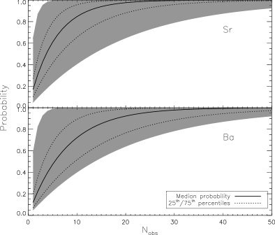
Despite the simplicity of our models, there are a number of interesting implications from our results. First, a relatively modest increase in the number of high-resolution spectra in UFDs could be used to test the specifics of our model — if our interpretation is correct (barring other effects), then we should find UFD members with abundance ratios skewed above the bulk of the MW distribution as well as below. Figure 12 illustrates the likelihood of finding at least one UFD star with positive values of either [Sr/Fe] (upper panel) or [Ba/Fe] (lower panel) for different sample sizes. The gray region indicates the full range of probabilities for all parameter sets for which we found p-values $\geq 0.05$ when compared to the current data sets in Sections 4.3 and 4.4. These probabilities were calculated from the parent distribution for each qualifying parameter set by finding the fraction of realizations, $f$, that had positive abundance ratios, and then adopting $f$ in the binomial theorem to estimate the probability of drawing at least one such star for sample size N_obs. The solid and dotted line indicates the median and $25^{th}$/$75^{th}$-percentiles for all qualifying parameters sets at a given N_obs. Overall, the figure indicates that, if our hypothesis of nc-abundance ratio distributions being skewed by strongly mass-dependent, power-law-like yields is a predominant effect, then sample sizes of $\sim$ 15 – 25 VMP stars in UFDs should start to contain some nc-rich ([Ba,Sr/Fe] $\gtrsim 0$) counterparts to the nc-poor ([Ba,Sr/Fe] $<0$) populations observed so far. Efforts made to extend stellar abundance ratio samples into the main sequence of UFDs (e.g. Vargas et al., 2013) should eventually provided samples large enough to determine whether stochastic sampling plays a predominant role in observed abundance ratio distributions.

Figure 12.— Gray region indicates the range in the probability that an observed UFD sample of size N_obs could contain one star with [Sr/Fe] $>0$ (top panel) or [Ba/Fe] $>0$ (bottom panel) for parameter sets that had $p$-values greater than 0.05 (see lower panels of Figures 10 and 11). The solid and dotted lines indicated the median and $25^{th}$/$75^{th}$-percentiles for these parameter sets, respectively.

Second, it should also be noted that as sample sizes increase, the likelihood distributions in our parameter space will become more concentrated, providing stronger constraints on the form of MDY for nc-elements, and, by extension, their origin. A preliminary comparison of our current results with predictions for MDY in literature already suggests that while production of Sr from $8-10M_{\odot}$ stars is quite possible, production of Ba from these stars is highly unlikely. Our results also support the viability of recent ab initio yields for $15-40M_{\odot}$ stars.

In conclusion, our results indicate that abundance ratio distributions in nearby systems contain intriguing signatures of their early isolation (or conversely, contamination): more/less isolated systems should be enriched by smaller/larger prior enriching generations (i.e. to have lower/higher $M_{\rm ESG}$). These signatures could potentially be exploited to probe the progress of metal enrichment on MW scales in the early Universe — a local window on a regime that cannot be seen directly.

Appendix A A    Effects of Varying the Upper Mass Limit

The plots in this appendix illustrate the results of adopting a different assumption for the high-mass cutoff of the IMF. Figure 13 repeats Figure 4 (left panels), adding panels for $m_{\rm upp}=60$ (middle panels) and 80 (right panels) to demonstrate how the yield distributions are affected across various $m_{\rm upp}$. As $m_{\rm upp}$ increases, the range in possible yields is increased, stretching the distribution in a similar manner to increasing $\kappa_{\rm X}$. While there is some noticeable degeneracy in the effects of $m_{\rm upp}$ and $\kappa_{\rm X}$ on skewness and in the effects of $m_{\rm upp}$ and $M_{\rm ESG}$ on dispersion, simple inspection suggests that the change in $m_{\rm upp}$ most strongly affects the kurtosis (peakedness) of the distribution. Increasing $m_{\rm upp}$ widens and flattens the distributions seen across the columns of Figure 13. Figure 14 displays a similar profile for negative MDYs.

Figure 13.— Distributions of abundance ratios produced from 1000 realizations of an ESG, with $M_{\rm ESG}=10^{2}M_{\odot}$ (top row), $10^{3}M_{\odot}$ (middle row), and $10^{4}M_{\odot}$ (bottom row). Each column represents models generated with different $m_{\rm upp}$ for the IMF: $40M_{\odot}$ (first column), $60M_{\odot}$ (second column), and $80M_{\odot}$ (third column). Colors are the same as found in Figure 4 of the paper.

Figure 14.— Figure is the similar to Figure 13 but shows distributions derived from negative MDYs.

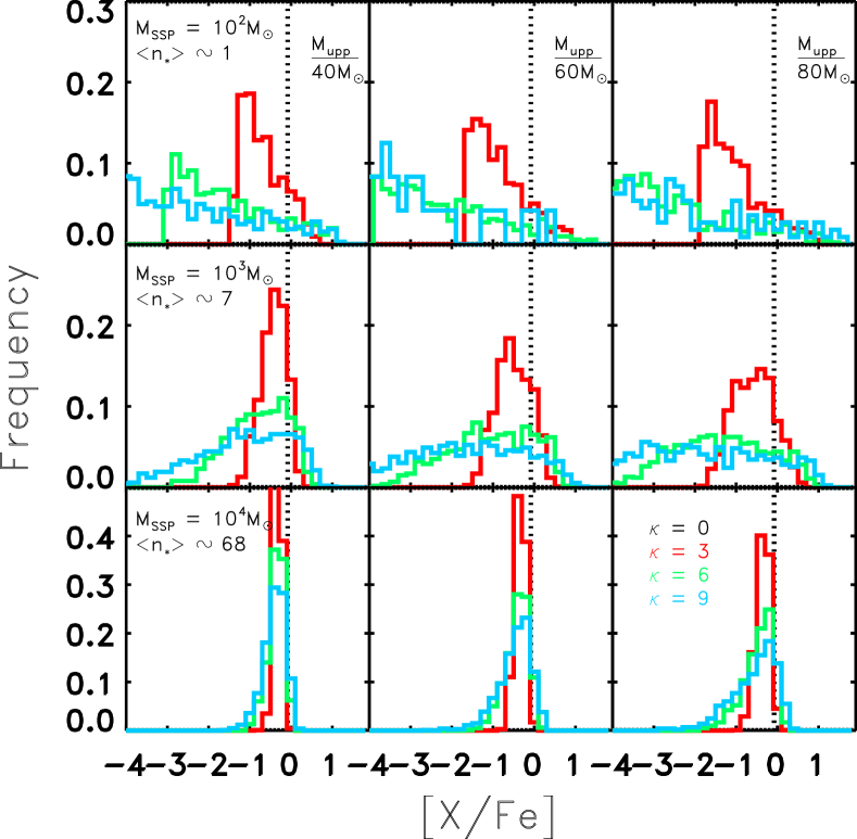
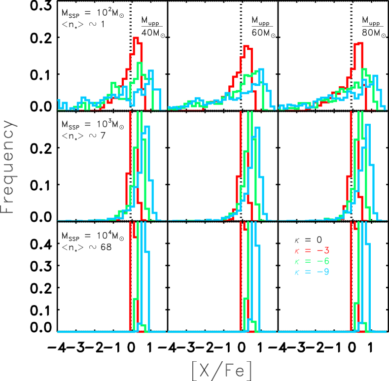
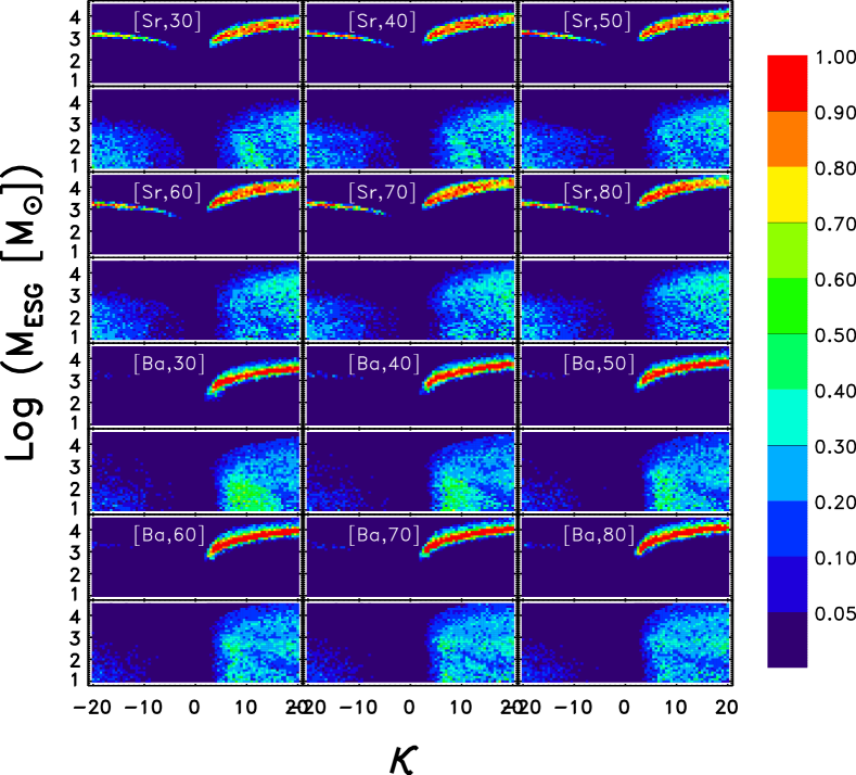
Figure 15 displays $p$-values from our paternal likelihood test for a variety of $m_{\rm upp}$ in both the [Ti/Fe]-[Sr/Fe] and [Ti/Fe]-[Ba/Fe] planes. As $m_{\rm upp}$ increases, our probability distributions shift to higher $M_{\rm ESG}$ values for a given $\kappa_{\rm X}$: the wider range of stellar masses means a wider range in individual SNe yields for a given $\kappa_{\rm X}$, requiring a larger $M_{\rm ESG}$ to match the observed abundance ratio spreads. However, the figure confirms that our general results - of the UFD distributions requiring large $|\kappa_{\rm X}|$ and smaller $M_{\rm ESG}$ than the MW distributions - are robust despite our ignorance of the actual value of $m_{\rm upp}$.

Figure 15.— Likelihoods (p-values) for all models examined as a function of $M_{\rm ESG}$, $\kappa_{\rm X}$, and $m_{\rm upp}$ for the two abundance ratio planes investigated. Models are indicated by a “Sr” for the [Ti/Fe]-[Sr/Fe] plane or a “Ba” for [Ti/Fe]-[Ba/Fe] plane and a value for $m_{\rm upp}$ in solar masses.

Appendix B B    Derivation of our MDY models

To create an analytic average abundance ratio from Eqn. (2), we first calculate a mass ratio in the limit of a completely sampled IMF:

$$\frac{M_{X}}{M_{Fe}} =\frac{\int_{m_{\rm enrich,low}}^{m_{\rm upp}}\!\xi\cdot m_{X}\,dm}{\int_{m_{\rm enrich,low}}^{m_{\rm upp}}\!\xi\cdot m_{Fe}\,dm}=\left(\frac{\beta_{\rm X}}{\beta_{\rm Fe}}\right)\cdot\left(\frac{\kappa_{\rm Fe}-\alpha+1}{\kappa_{\rm X}-\alpha+1}\right)\cdot\left(\frac{{m_{\rm upp}}^{\kappa_{\rm X}-\alpha+1}-{m_{\rm enrich,low}}^{\kappa_{\rm X}-\alpha+1}}{{m_{\rm upp}}^{\kappa_{\rm Fe}-\alpha+1}-{m_{\rm enrich,low}}^{\kappa_{\rm Fe}-\alpha+1}}\right)$$ (B1)

where M_X and M_Fe represent the total mass yield in X and Fe.

We can relate Eqn. (B1) to solar abundance ratios and thereby calculate the IMF-weighted chemical abundance ratio [X/Fe]:

$$\left[\frac{\rm X}{\rm Fe}\right]_{\rm IMF}\equiv \log\left(\frac{M_{X}}{M_{Fe}}\right)-\log\left(\frac{M_{mol}(X)}{M_{mol}(Fe)}\right)-\log\left(\frac{N_{X,\odot}}{N_{Fe,\odot}}\right)$$ (B2)

where $\left[\frac{\rm X}{\rm Fe}\right]_{\rm IMF}$ is the IMF-weighted abundance ratio, $\frac{M_{mol}(X)}{M_{mol}(Fe)}$ is a ratio of the molar masses of X and Fe, and $\frac{N_{X,\odot}}{N_{Fe,\odot}}$ is the ratio of the solar abundances of X and Fe. We can then use the average of observed abundance ratios from our sample of MW halo stars, $\left<\left[\frac{\rm X}{\rm Fe}\right]\right>_{\rm OBS}$, to calibrate $\beta$ for a given $\kappa_{\rm X}$ of element X by using Eqn. 3.

References

- Abadi et al. (2003a) Abadi, M. G., Navarro, J. F., Steinmetz, M., & Eke, V. R. 2003a, ApJ, 591, 499
- Abadi et al. (2003b) —. 2003b, ApJ, 597, 21
- Aoki et al. (2007) Aoki, W., Beers, T. C., Christlieb, N., Norris, J. E., Ryan, S. G., & Tsangarides, S. 2007, ApJ, 655, 492
- Audouze & Silk (1995) Audouze, J., & Silk, J. 1995, ApJ, 451, L49
- Babu & Feigelson (2006) Babu, G. J., & Feigelson, E. D. 2006, in Astronomical Society of the Pacific Conference Series, Vol. 351, Astronomical Data Analysis Software and Systems XV, ed. C. Gabriel, C. Arviset, D. Ponz, & S. Enrique, 127
- Babu & Rao (2004) Babu, G. J., & Rao, C. R. 2004, Sankhyā: The Indian Journal of Statistics (2003-2007), 66, pp. 63
- Beers & Christlieb (2005) Beers, T. C., & Christlieb, N. 2005, ARA&A, 43, 531
- Bell et al. (2008) Bell, E. F. et al. 2008, ApJ, 680, 295
- Bland-Hawthorn et al. (2010) Bland-Hawthorn, J., Karlsson, T., Sharma, S., Krumholz, M., & Silk, J. 2010, ApJ, 721, 582
- Boffin & Jorissen (1988) Boffin, H. M. J., & Jorissen, A. 1988, A&A, 205, 155
- Bullock & Johnston (2005) Bullock, J. S., & Johnston, K. V. 2005, ApJ, 635, 931
- Carigi & Hernandez (2008) Carigi, L., & Hernandez, X. 2008, MNRAS, 390, 582
- Cescutti (2012) Cescutti, G. 2012, in Chemical Evolution of the Milky Way
- Cescutti & Chiappini (2013) Cescutti, G., & Chiappini, C. 2013, ArXiv e-prints
- Chabrier (2003) Chabrier, G. 2003, Publ.Astron.Soc.Pac., 115, 763
- Chiappini et al. (2011) Chiappini, C., Frischknecht, U., Meynet, G., Hirschi, R., Barbuy, B., Pignatari, M., Decressin, T., & Maeder, A. 2011, Nature, 472, 454
- Chieffi & Limongi (2004) Chieffi, A., & Limongi, M. 2004, ApJ, 608, 405
- Cooper et al. (2010) Cooper, A. P. et al. 2010, MNRAS, 406, 744
- Corlies et al. (2013) Corlies, L., Johnston, K. V., Tumlinson, J., & Bryan, G. 2013, ArXiv e-prints
- Eggen et al. (1962) Eggen, O. J., Lynden-Bell, D., & Sandage, A. R. 1962, ApJ, 136, 748
- Elmegreen (2006) Elmegreen, B. G. 2006, ArXiv Astrophysics e-prints
- Elmegreen (2007) Elmegreen, B. G. 2007, in Astronomical Society of the Pacific Conference Series, Vol. 362, The Seventh Pacific Rim Conference on Stellar Astrophysics, ed. Y. W. Kang, H.-W. Lee, K.-C. Leung, & K.-S. Cheng, 269
- Elmegreen & Scalo (2005) Elmegreen, B. G., & Scalo, J. 2005, Astrophys.J., 636, 149
- Fasano & Franceschini (1987) Fasano, G., & Franceschini, A. 1987, MNRAS, 225, 155
- Fischer et al. (2010) Fischer, T., Whitehouse, S. C., Mezzacappa, A., Thielemann, F.-K., & Liebendörfer, M. 2010, A&A, 517, A80
- Font et al. (2006) Font, A. S., Johnston, K. V., Bullock, J. S., & Robertson, B. E. 2006, ApJ, 638, 585
- Frebel (2010) Frebel, A. 2010, Astronomische Nachrichten, 331, 474
- Frebel & Bromm (2012) Frebel, A., & Bromm, V. 2012, ApJ, 759, 115
- Frebel et al. (2010) Frebel, A., Simon, J. D., Geha, M., & Willman, B. 2010, ApJ, 708, 560
- Frischknecht et al. (2012) Frischknecht, U., Hirschi, R., & Thielemann, F.-K. 2012, A&A, 538, L2
- Geisler et al. (2007) Geisler, D., Wallerstein, G., Smith, V. V., & Casetti-Dinescu, D. I. 2007, PASP, 119, 939
- Heger & Woosley (2010) Heger, A., & Woosley, S. E. 2010, ApJ, 724, 341
- Herwig (2005) Herwig, F. 2005, ARA&A, 43, 435
- Hoeft et al. (2006) Hoeft, M., Yepes, G., Gottlöber, S., & Springel, V. 2006, MNRAS, 371, 401
- Ishimaru & Wanajo (1999) Ishimaru, Y., & Wanajo, S. 1999, ApJ, 511, L33
- Karlsson (2005) Karlsson, T. 2005, A&A, 439, 93
- Karlsson & Gustafsson (2005) Karlsson, T., & Gustafsson, B. 2005, A&A, 436, 879
- Koch (2009) Koch, A. 2009, Astronomische Nachrichten, 330, 675
- Kroupa (2002) Kroupa, P. 2002, Science, 295, 82
- Limongi & Chieffi (2012) Limongi, M., & Chieffi, A. 2012, ApJS, 199, 38
- Mathews et al. (1992) Mathews, G. J., Bazan, G., & Cowan, J. J. 1992, ApJ, 391, 719
- Mayer et al. (2006) Mayer, L., Mastropietro, C., Wadsley, J., Stadel, J., & Moore, B. 2006, MNRAS, 369, 1021
- McCarthy et al. (2012) McCarthy, I. G., Font, A. S., Crain, R. A., Deason, A. J., Schaye, J., & Theuns, T. 2012, MNRAS, 420, 2245
- McClure & Woodsworth (1990) McClure, R. D., & Woodsworth, A. W. 1990, ApJ, 352, 709
- McWilliam (1997) McWilliam, A. 1997, ARA&A, 35, 503
- McWilliam (1998) —. 1998, AJ, 115, 1640
- Nomoto et al. (2006) Nomoto, K., Tominaga, N., Umeda, H., Kobayashi, C., & Maeda, K. 2006, Nuclear Physics A, 777, 424
- Norris et al. (2000) Norris, J. E., Beers, T. C., & Ryan, S. G. 2000, ApJ, 540, 456
- Norris et al. (2010) Norris, J. E., Yong, D., Gilmore, G., & Wyse, R. F. G. 2010, ApJ, 711, 350
- Peacock (1983) Peacock, J. A. 1983, MNRAS, 202, 615
- Press (1992) Press, W. H. 1992, Numerical recipes in C: the art of scientific computing, 2nd edn. (Cambridge: Cambridge University Press)
- Qian & Wasserburg (2008) Qian, Y.-Z., & Wasserburg, G. J. 2008, ApJ, 687, 272
- Robertson et al. (2005) Robertson, B., Bullock, J. S., Font, A. S., Johnston, K. V., & Hernquist, L. 2005, ApJ, 632, 872
- Roederer (2013) Roederer, I. U. 2013, AJ, 145, 26
- Roederer et al. (2010) Roederer, I. U., Cowan, J. J., Karakas, A. I., Kratz, K.-L., Lugaro, M., Simmerer, J., Farouqi, K., & Sneden, C. 2010, ApJ, 724, 975
- Ryan et al. (1996) Ryan, S. G., Norris, J. E., & Beers, T. C. 1996, ApJ, 471, 254
- Salpeter (1955) Salpeter, E. E. 1955, ApJ, 121, 161
- Schlaufman et al. (2009) Schlaufman, K. C. et al. 2009, ApJ, 703, 2177
- Searle & Zinn (1978) Searle, L., & Zinn, R. 1978, ApJ, 225, 357
- Shetrone et al. (2003) Shetrone, M., Venn, K. A., Tolstoy, E., Primas, F., Hill, V., & Kaufer, A. 2003, AJ, 125, 684
- Simon et al. (2010) Simon, J. D., Frebel, A., McWilliam, A., Kirby, E. N., & Thompson, I. B. 2010, ApJ, 716, 446
- Smith & Lambert (1990) Smith, V. V., & Lambert, D. L. 1990, ApJS, 72, 387
- Stephens (1974) Stephens, M. A. 1974, Journal of the American Statistical Association, 69, pp. 730
- Tissera et al. (2012) Tissera, P. B., White, S. D. M., & Scannapieco, C. 2012, MNRAS, 420, 255
- Tolstoy et al. (2009) Tolstoy, E., Hill, V., & Tosi, M. 2009, ARA&A, 47, 371
- Tumlinson (2006) Tumlinson, J. 2006, ApJ, 641, 1
- Vargas et al. (2013) Vargas, L. C., Geha, M., Kirby, E. N., & Simon, J. D. 2013
- Venn et al. (2004) Venn, K. A., Irwin, M., Shetrone, M. D., Tout, C. A., Hill, V., & Tolstoy, E. 2004, AJ, 128, 1177
- Wanajo et al. (2011) Wanajo, S., Janka, H.-T., & Müller, B. 2011, ApJ, 726, L15
- Wanajo et al. (2003) Wanajo, S., Tamamura, M., Itoh, N., Nomoto, K., Ishimaru, Y., Beers, T. C., & Nozawa, S. 2003, ApJ, 593, 968
- Wheeler et al. (1998) Wheeler, J. C., Cowan, J. J., & Hillebrandt, W. 1998, ApJ, 493, L101
- Xue et al. (2011) Xue, X.-X. et al. 2011, ApJ, 738, 79
- Zolotov et al. (2010) Zolotov, A., Willman, B., Brooks, A. M., Governato, F., Hogg, D. W., Shen, S., & Wadsley, J. 2010, ApJ, 721, 738