Tractable Combinations of Global Constraints

Abstract

We study the complexity of constraint satisfaction problems involving global constraints, i.e., special-purpose constraints provided by a solver and represented implicitly by a parametrised algorithm. Such constraints are widely used; indeed, they are one of the key reasons for the success of constraint programming in solving real-world problems.

Previous work has focused on the development of efficient propagators for individual constraints. In this paper, we identify a new tractable class of constraint problems involving global constraints of unbounded arity. To do so, we combine structural restrictions with the observation that some important types of global constraint do not distinguish between large classes of equivalent solutions.

1 Introduction

Constraint programming (CP) is widely used to solve a variety of practical problems such as planning and scheduling [23, 30], and industrial configuration [1, 22]. The theoretical properties of constraint problems, in particular the computational complexity of different types of problem, have been extensively studied and quite a lot is known about what restrictions on the general constraint satisfaction problem are sufficient to make it tractable [2, 7, 11, 17, 20, 25].

However, much of this theoretical work has focused on problems where each constraint is represented explicitly, by a table of allowed assignments.

In practice, however, a lot of the success of CP is due to the use of special-purpose constraint types for which the software tools provide dedicated algorithms [28, 16, 31]. Such constraints are known as global constraints and are usually represented implicitly by an algorithm in the solver. This algorithm may take as a parameter a description that specifies exactly which kinds of assignments a particular instance of this constraint should allow.

Theoretical work on global constraints has to a large extent focused on developing efficient algorithms to achieve various kinds of local consistency for individual constraints. This is generally done by pruning from the domains of variables those values that cannot lead to a satisfying assignment [5, 29]. Another strand of research has explored when it is possible to replace global constraints by collections of explicitly represented constraints [6]. These techniques allow faster implementations of algorithms for individual constraints, but do not shed much light on the complexity of problems with multiple overlapping global constraints, which is something that practical problems frequently require.

As an example, consider the following family of constraint problems involving clauses and cardinality constraints of unbounded arity.

Example 1

Consider a family of constraint problems on a set of Boolean variables $\{x_{1},x_{2},\ldots,x_{3n}\}$ (where $n=2,3,4,\ldots$), with the following five constraints:

• $C_{1}$ is the binary clause $x_{1}\vee x_{2n+1}$;

• $C_{2}$ is a cardinality constraint on $\{x_{1},x_{2},\ldots,x_{n}\}$ specifying that exactly one of these variables takes the value 1;

• $C_{3}$ is a cardinality constraint on $\{x_{2n+1},x_{2n+2},\ldots,x_{3n}\}$ specifying that exactly one of these variables takes the value 1;

• $C_{4}$ is a cardinality constraint on $\{x_{2},x_{3},\ldots,x_{3n}\}-\{x_{2n+1}\}$ specifying that exactly $n+1$ of these variables takes the value 1;

• $C_{5}$ is the clause $\neg x_{n+1}\vee\neg x_{n+2}\vee\cdots\vee\neg x_{2n}$.

This problem is illustrated in Figure 1.

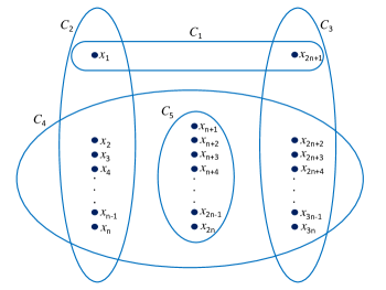
Figure 1: The structure of the constraint problems in Example 1

This family of problems is not included in any previously known tractable class, but will be shown to be tractable using the results of this paper.

As discussed in [9], when the constraints in a family of problems have unbounded arity, the way that the constraints are represented can significantly affect the complexity. Previous work in this area has assumed that the global constraints have specific representations, such as propagators [19], negative constraints [10], or GDNF/decision diagrams [9], and exploited properties particular to that representation. In contrast, here we investigate the conditions that yield efficiently solvable classes of constraint problems with global constraints, without requiring any specific representation. Many global constraints have succinct representations, so even problems with very simple structures are known to be hard in some cases [24, 29]. We will therefore need to impose some restrictions on the properties of the individual global constraints, as well as on the problem structure.

To obtain our results, we define a notion of equivalence on assignments and a new width measure that identifies variables that are constrained in exactly the same way. We then show that we can replace variables that are equated under our width measure with a single new variable whose domain represents the possible equivalence classes of assignments. Both of these simplification steps, merging variables and equating assignments, can be seen as techniques for eliminating symmetries in the original problem formulation. We describe some sufficient conditions under which these techniques provide a polynomial-time reduction to a known tractable case, and hence identify new tractable classes of constraint problems involving global constraints.

2 Global Constraints and Constraint Problems

In order to be more precise about the way in which global constraints are represented, we will extend the standard definition of a constraint problem.

Definition 1 (Variables and assignments)

Let $V$ be a set of variables, each with an associated set of domain elements. We denote the set of domain elements (the domain) of a variable $v$ by $D(v)$. We extend this notation to arbitrary subsets of variables, $W$, by setting $D(W)=\displaystyle\bigcup_{v\in W}D(v)$.

An assignment of a set of variables $V$ is a function $\theta:V\rightarrow D(V)$ that maps every $v\in V$ to an element $\theta(v)\in D(v)$. We denote the restriction of $\theta$ to a set of variables $W\subseteq V$ by $\theta|_{W}$. We also allow the special assignment $\bot$ of the empty set of variables. In particular, for every assignment $\theta$, we have $\theta|_{\emptyset}=\bot$.

Global constraints have traditionally been defined, somewhat vaguely, as constraints without a fixed arity, possibly also with a compact representation of the constraint relation. For example, in [23] a global constraint is defined as “a constraint that captures a relation between a non-fixed number of variables”.

Below, we offer a precise definition similar to the one in [5], where the authors define global constraints for a domain $D$ over a list of variables $\sigma$ as being given intensionally by a function $D^{|\sigma|}\rightarrow\{0,1\}$ computable in polynomial time. Our definition differs from this one in that we separate the general algorithm of a global constraint (which we call its type) from the specific description. This separation allows us a better way of measuring the size of a global constraint, which in turn helps us to establish new complexity results.

Definition 2 (Global constraints)

A global constraint type is a parametrised polynomial-time algorithm that determines the acceptability of an assignment of a given set of variables.

Each global constraint type, $e$, has an associated set of descriptions, $\Delta(e)$. Each description $\delta\in\Delta(e)$ specifies appropriate parameter values for the algorithm $e$. In particular, each $\delta\in\Delta(e)$ specifies a set of variables, denoted by $\mathsf{vars}(\delta)$.

A global constraint $e[\delta]$, where $\delta\in\Delta(e)$, is a function that maps assignments of $\mathsf{vars}(\delta)$ to the set $\{0,1\}$. Each assignment that is allowed by $e[\delta]$ is mapped to 1, and each disallowed assignment is mapped to 0. The extension or constraint relation of $e[\delta]$ is the set of assignments, $\theta$, of $\mathsf{vars}(\delta)$ such that $e[\delta](\theta)=1$. We also say that such assignments satisfy the constraint, while all other assignments falsify it.

When we are only interested in describing the set of assignments that satisfy a constraint, and not in the complexity of determining membership in this set, we will sometimes abuse notation by writing $\theta\in e[\delta]$ to mean $e[\delta](\theta)=1$.

As can be seen from the definition above, a global constraint is not usually explicitly represented by listing all the assignments that satisfy it. Instead, it is represented by some description $\delta$ and some algorithm $e$ that allows us to check whether the constraint relation of $e[\delta]$ includes a given assignment. To stay within the complexity class , this algorithm is required to run in polynomial time. As the algorithms for many common global constraints are built into modern constraint solvers, we measure the size of a global constraint’s representation by the size of its description.

Example 2 (EGC)

A very general global constraint type is the extended global cardinality constraint type [26, 29]. This form of global constraint is defined by specifying for every domain element $a$ a finite set of natural numbers $K(a)$, called the cardinality set of $a$. The constraint requires that the number of variables which are assigned the value $a$ is in the set $K(a)$, for each possible domain element $a$.

Using our notation, the description $\delta$ of an EGC global constraint specifies a function $K_{\delta}:D(\mathsf{vars}(\delta))\rightarrow\mathcal{P}(\mathbb{N})$ that maps each domain element to a set of natural numbers. The algorithm for the EGC constraint then maps an assignment $\theta$ to $1$ if and only if, for every domain element $a\in D(\mathsf{vars}(\delta))$, we have that $|\{v\in\mathsf{vars}(\delta)\mid\theta(v)=a\}|\in K_{\delta}(a)$.

The cardinality constraint $C_{2}$ from Example 1 can be expressed as an EGC global constraint with description $\delta$ such that $K_{\delta}(1)=\{1\}$, and $K_{\delta}(0)=\{n-1\}$.

Example 3 (Clauses)

We can view the disjunctive clauses used to define propositional satisfiability problems as a global constraint type in the following way.

The description $\delta$ of a clause is simply a list of the literals that it contains, and $\mathsf{vars}(\delta)$ is the corresponding set of variables. The algorithm for the clause then maps any Boolean assignment $\theta$ of $\mathsf{vars}(\delta)$ that satisfies the disjunction of the literals specified by $\delta$ to 1, and all other assignments to 0.

Note that a clause forbids precisely one assignment to $\mathsf{vars}(\delta)$ (the one that falsifies all of the literals in the clause). Hence the extension of a clause contains $2^{|\mathsf{vars}(\delta)|}-1$ assignments, so the size of the constraint relation grows exponentially with the number of variables, but the size of the constraint description grows only linearly.

Example 4 (Table and negative constraints)

A rather degenerate example of a a global constraint type is the table constraint.

In this case the description $\delta$ is simply a list of assignments of some fixed set of variables, $\mathsf{vars}(\delta)$. The algorithm for a table constraint then decides, for any assignment of $\mathsf{vars}(\delta)$, whether it is included in $\delta$. This can be done in a time which is linear in the size of $\delta$ and so meets the polynomial time requirement.

Negative constraints are complementary to table constraints, in that they are described by listing forbidden assignments. The algorithm for a negative constraint $e[\delta]$ decides, for any assignment of $\mathsf{vars}(\delta)$, whether it is not included in $\delta$. Observe that the clauses described in Example 3 are a special case of the negative constraint type, as they have exactly one forbidden assignment.

We observe that any global constraint can be rewritten as a table or negative constraint. However, this rewriting will, in general, incur an exponential increase in the size of the description.

Definition 3 (CSP instance)

An instance of the constraint satisfaction problem (CSP) is a pair $\langle V,C\rangle$ where $V$ is a finite set of variables, and $C$ is a set of global constraints such that for every $e[\delta]\in C$, $\mathsf{vars}(\delta)\subseteq V$. In a CSP instance, we call $\mathsf{vars}(\delta)$ the scope of the constraint $e[\delta]$.

A solution to a CSP instance $\langle V,C\rangle$ is an assignment $\theta$ of $V$ which satisfies every global constraint, i.e., for every $e[\delta]\in C$ we have $\theta|_{\mathsf{vars}(\delta)}\in e[\delta]$.

The general constraint satisfaction problem is clearly NP-complete, so in the remainder of the paper we shall look for more restricted versions of the problem that are tractable, that is, solvable in polynomial time.

3 Restricted Classes of Constraint Problems

First, we are going to consider restrictions on the way that the constraints in a given instance interact with each other, or, in other words, the way that the constraint scopes overlap; such restrictions are known as structural restrictions [11, 17, 20].

Definition 4 (Hypergraph)

A hypergraph $\langle V,H\rangle$ is a set of vertices $V$ together with a set of hyperedges $H\subseteq\mathcal{P}(V)$.

Given a CSP instance $P=\langle V,C\rangle$, the hypergraph of $P$, denoted $\mathsf{hyp}(P)$, has vertex set $V$ together with a hyperedge $\mathsf{vars}(\delta)$ for every $e[\delta]\in C$.

One special class of hypergraphs that has received a great deal of attention is the class of acyclic hypergraphs [3]. This notion is a generalisation of the idea of tree-structure in a graph, and has been very important in the analysis of relational databases. A hypergraph is said to be acyclic if repeatedly removing all hyperedges contained in other hyperedges, and all vertices contained in only a single hyperedge, eventually deletes all vertices [3].

Solving a CSP instance $P$ whose constraints are represented extensionally (i.e., as table constraints) is known to be tractable if the hypergraph of $P$, $\mathsf{hyp}(P)$, is acyclic [21]. Indeed, this has formed the basis for more general notions of “bounded cyclicity” [21] or “bounded hypertree width” [18], which have also been shown to imply tractability for problems with explicitly represented constraint relations. However, this is no longer true if the constraints are global, not even when we have a fixed, finite domain, as the following examples show.

Example 5

Any hypergraph containing only a single edge is clearly acyclic (and therefore has hypertree width one [18]), but the class of CSP instances consisting of a single EGC constraint over an unbounded domain is -complete [26].

Example 6

The -complete problem of 3-colourability [15] is to decide, given a graph $\langle V,E\rangle$, whether the vertices $V$ can be coloured with three colours such that no two adjacent vertices have the same colour.

We may reduce this problem to a CSP with EGC constraints (cf. Example 2) as follows: Let $V$ be the set of variables for our CSP instance, each with domain $\{r,g,b\}$. For every edge $\langle v,w\rangle\in E$, we post an EGC constraint with scope $\{v,w\}$, parametrised by the function $K$ such that $K(r)=K(g)=K(b)=\{0,1\}$. Finally, we make the hypergraph of this CSP instance acyclic by adding an EGC constraint with scope $V$ parametrised by the function $K^{\prime}$ such that $K^{\prime}(r)=K^{\prime}(g)=K^{\prime}(b)=\{0,\ldots,|V|\}$. This reduction clearly takes polynomial time, and the hypergraph of the resulting instance is acyclic.

These examples indicate that when dealing with implicitly represented constraints we cannot hope for tractability using structural restrictions alone. We are therefore led to consider hybrid restrictions, which restrict both the nature of the constraints and the structure at the same time.

Definition 5 (Constraint catalogue)

A constraint catalogue is a set of global constraints. A CSP instance $\langle V,C\rangle$ is said to be over a constraint catalogue $\mathcal{C}$ if for every $e[\delta]\in C$ we have $e[\delta]\in\mathcal{C}$.

Previous work on the complexity of constraint problems has restricted the extensions of the constraints to a specified set of relations, known as a constraint language [7]. This is an appropriate form of restriction when all constraints are given explicitly, as table constraints. However, here we work with global constraints where the relations are often implicit, and this can significantly alter the complexity of the corresponding problem classes, as we will illustrate below. Hence we allow a more general form of restriction on the constraints by specifying a constraint catalogue containing all allowed constraints.

Definition 6 (Restricted CSP class)

Let $\mathcal{C}$ be a constraint catalogue, and let $\mathcal{H}$ be a class of hypergraphs. We define $\mathsf{CSP}(\mathcal{H},\mathcal{C})$ to be the class of CSP instances over $\mathcal{C}$ whose hypergraphs are in $\mathcal{H}$.

Using Definition 6, we will restate an earlier structural tractability result, which will form the basis for our results in Section 5.

Definition 7 (Treewidth)

A tree decomposition of a hypergraph $\langle V,H\rangle$ is a pair $\langle T,\lambda\rangle$ where $T$ is a tree and $\lambda$ is a labelling function from nodes of $T$ to subsets of $V$, such that

1. for every $v\in V$, there exists a node $t$ of $T$ such that $v\in\lambda(t)$,

2. for every hyperedge $h\in E$, there exists a node $t$ of $T$ such that $h\subseteq\lambda(t)$, and

3. for every $v\in V$, the set of nodes $\{t\mid v\in\lambda(t)\}$ induces a connected subtree of $T$.

The width of a tree decomposition is $\max(\{|\lambda(t)|-1\mid t\mbox{ node of }T\})$. The treewidth $\mathsf{tw}(G)$ of a hypergraph $G$ is the minimum width over all its tree decompositions.

Let $\mathcal{H}$ be a class of hypergraphs, and define $\mathsf{tw}(\mathcal{H})$ to be the maximum treewidth over the hypergraphs in $\mathcal{H}$. If $\mathsf{tw}(\mathcal{H})$ is unbounded we write $\mathsf{tw}(\mathcal{H})=\infty$; otherwise $\mathsf{tw}(\mathcal{H})<\infty$.

We can now restate using the language of global constraints the following result, from Dalmau et al. [12], which builds on several earlier results [13, 14].

Theorem 3.1 ([12])

Let $\mathcal{C}$ be a constraint catalogue and $\mathcal{H}$ a class of hypergraphs. $\mathsf{CSP}(\mathcal{H},\mathcal{C})$ is tractable if $\mathsf{tw}(\mathcal{H})<\infty$.

Observe that the family of constraint problems described in Example 1 is not covered by the above result, because the treewidth of the associated hypergraphs is unbounded.

4 Cooperating Constraint Catalogues

Whenever constraint scopes overlap, we may ask whether the possible assignments to the variables in the overlap are essentially different. It may be that some assignments extend to precisely the same satisfying assignments in each of the overlapping constraints. If so, we may as well identify such assignments.

Definition 8 (Disjoint union of assignments)

Let $\theta_{1}$ and $\theta_{2}$ be two assignments of disjoint sets of variables $V_{1}$ and $V_{2}$, respectively. The disjoint union of $\theta_{1}$ and $\theta_{2}$, denoted $\theta_{1}\oplus\theta_{2}$, is the assignment of $V_{1}\cup V_{2}$ such that $(\theta_{1}\oplus\theta_{2})(v)=\theta_{1}(v)$ for all $v\in V_{1}$, and $(\theta_{1}\oplus\theta_{2})(v)=\theta_{2}(v)$ for all $v\in V_{2}$.

Definition 9 (Projection)

Let $\Theta$ be a set of assignments of a set of variables $V$. The projection of $\Theta$ onto a set of variables $X\subseteq V$ is the set of assignments $\pi_{X}(\Theta)=\{\theta|_{X}\mid\theta\in\Theta\}$.

Note that when $\Theta=\emptyset$ we have $\pi_{X}(\Theta)=\emptyset$ for any set $X$, but when $X=\emptyset$ and $\Theta\neq\emptyset$, we have $\pi_{X}(\Theta)=\{\bot\}$.

Definition 10 (Assignment extension)

Let $e[\delta]$ be a global constraint, and $X\subseteq\mathsf{vars}(\delta)$. For every assignment $\mu$ of $X$, let $\mathsf{ext}(\mu,e[\delta])=\pi_{\mathsf{vars}(\delta)-X}(\{\theta\in e[\delta]\mid\theta|_{X}=\mu\})$.

In other words, for any assignment $\mu$ of $X$, the set $\mathsf{ext}(\mu,e[\delta])$ is the set of assignments of $\mathsf{vars}(\delta)-X$ that extend $\mu$ to a satisfying assignment for $e[\delta]$; i.e., those assignments $\theta$ for which $\mu\oplus\theta\in e[\delta]$.

Definition 11 (Extension equivalence)

Let $e[\delta]$ be a global constraint, and $X\subseteq\mathsf{vars}(\delta)$. We say that two assignments $\theta_{1},\theta_{2}$ to $X$ are extension equivalent on $X$ with respect to $e[\delta]$ if $\mathsf{ext}(\theta_{1},e[\delta])=\mathsf{ext}(\theta_{2},e[\delta])$. We denote this equivalence relation by $\mathsf{equiv}[e[\delta],X]$; that is, $\mathsf{equiv}[e[\delta],X](\theta_{1},\theta_{2})$ holds if and only if $\theta_{1}$ and $\theta_{2}$ are extension equivalent on $X$ with respect to $e[\delta]$.

In other words, two assignments to some subset of the variables of a constraint $e[\delta]$ are extension equivalent if every assignment to the rest of the variables combines with both of them to give either two assignments that satisfy $e[\delta]$, or two that falsify it.

Example 7

Consider the special case of extension equivalence with respect to a clause (cf. Example 3).

Given any clause $e[\delta]$, and any non-empty set of variables $X\subseteq\mathsf{vars}(\delta)$, any assignment to $X$ will either satisfy one of the corresponding literals specified by $\delta$, or else falsify all of them. If it satisfies at least one of them, then any extension will satisfy the clause, so all such assignments are extension equivalent. If it falsifies all of them, then an extension will satisfy the clauses if and only if it satifies one of the other literals. Hence the equivalence relation $\mathsf{equiv}[e[\delta],X]$ has precisely 2 equivalence classes, one containing the single assignment that falsifies all the literals corresponding to X, and one containing all other assignments.

Definition 12 (Intersecting variables)

Let $S$ be a set of global constraints. We write $\mathsf{iv}(S)$ for the set of variables common to all of their scopes, that is, $\mathsf{iv}(S)=\displaystyle\bigcap_{e[\delta]\in S}\mathsf{vars}(\delta)$.

Definition 13 (Join)

For any set $S$ of global constraints, we define the join of $S$, denoted $\mathsf{join}(S)$, to be a global constraint $e^{\prime}[\delta^{\prime}]$ with $\mathsf{vars}(\delta^{\prime})=\displaystyle\bigcup_{e[\delta]\in S}\mathsf{vars}(\delta)$ such that for any assignment $\theta$ to $\mathsf{vars}(\delta^{\prime})$, we have $\theta\in e^{\prime}[\delta^{\prime}]$ if and only if for every $e[\delta]\in S$ we have $\theta|_{\mathsf{vars}(\delta)}\in e[\delta]$.

The join of a set of global constraints may have no simple compact description, and computing its extension may be computationally expensive. However, we introduce this construct simply in order to describe the combined effect of a set of global constraints in terms of a single constraint.

Example 8

Let $V=\{v_{1},\ldots,v_{n}\}$, for some $n\geq 3$, be a set of variables with $D(v_{i})=\{a,b,c\}$, and let $S=\{e_{1}[\delta_{1}],e_{2}[\delta_{2}]\}$ be a set of two global constraints as defined below:

• $e_{1}[\delta_{1}]$ is a table constraint with $\mathsf{vars}(\delta_{1})=\{v_{1},\ldots,v_{n-1}\}$ which enforces equality, i.e., $\delta_{1}=\{\theta_{a},\theta_{b},\theta_{c}\}$, where for each $x\in D(V)$ and $v\in\mathsf{vars}(\delta_{1})$, $\theta_{x}(v)=x$.

• $e_{2}[\delta_{2}]$ is a negative constraint with $\mathsf{vars}(\delta_{2})=\{v_{2},\ldots,v_{n}\}$ which enforces a not-all-equal condition, i.e., $\delta_{2}=\{\theta_{a},\theta_{b},\theta_{c}\}$, where for each $x\in D(V)$ and $v\in\mathsf{vars}(\delta_{2})$, $\theta_{x}(v)=x$.

We will use substitution notation to write assignments explicitly; thus, an assignment of $\{v,w\}$ that assigns $a$ to both variables is written $\{v/a,w/a\}$.

We have that $\mathsf{iv}(S)=\{v_{2},\ldots,v_{n-1}\}$. The equivalence classes of assignments to $\mathsf{iv}(S)$ under $\mathsf{equiv}[\mathsf{join}(S),\mathsf{iv}(S)]$ are $\{\{v_{2}/a,\ldots,v_{n-1}/a\}\}$, $\{\{v_{2}/b,\ldots,v_{n-1}/b\}\}$, and $\{\{v_{2}/c,\ldots,v_{n-1}/c\}\}$, each containing the single assignment shown, as well as (for $n>3$) a final class containing all other assignments, for which we can choose an arbitrary representative assignment, $\theta_{0}$, such as $\{v_{2}/a,v_{3}/b,\ldots,v_{n-1}/b\}$.

Each assignment in the first 3 classes has just 2 possible extensions that satisfy $\mathsf{join}(S)$, since the value assigned to $v_{1}$ must equal the value assigned to $v_{2},\ldots,v_{n-1}$, and the value assigned to $v_{n}$ must be different. The assignment $\theta_{0}$ has no extensions, since $\mathsf{ext}(\theta_{0},e_{1}[\delta_{1}])=\emptyset$.

Hence the number of equivalence classes in $\mathsf{equiv}[\mathsf{join}(S),\mathsf{iv}(S)]$ is at most 4, even though the total number of possible assignments of $\mathsf{iv}(S)$ is $3^{n-2}$

Definition 14 (Cooperating constraint catalogue)

We say that a constraint catalogue $\mathcal{C}$ is a cooperating catalogue if for any finite set of global constraints $S\subseteq\mathcal{C}$, we can compute a set of assignments of the variables $\mathsf{iv}(S)$ containing at least one representative of each equivalence class of $\mathsf{equiv}[\mathsf{join}(S),\mathsf{iv}(S)]$ in polynomial time in the size of $\mathsf{iv}(S)$ and the total size of the constraints in $S$.

Note that this definition requires two things. First, that the number of equivalence classes in the equivalence relation $\mathsf{equiv}[\mathsf{join}(S),\mathsf{iv}(S)]$ is bounded by some fixed polynomial in the size of $\mathsf{iv}(S)$ and the size of the constraints in $S$. Secondly, that a suitable set of representatives for these equivalence classes can be computed efficiently from the constraints.

Example 9

Consider a constraint catalogue consisting entirely of clauses (of arbitrary arity). It was shown in Example 7 that for any clause $e[\delta]$ and any non-empty $X\subseteq\mathsf{vars}(\delta)$ the equivalence relation $\mathsf{equiv}[e[\delta],X]$ has precisely 2 equivalence classes.

If we consider some finite set, $S$, of clauses, then a similar argument shows that the equivalence relation $\mathsf{equiv}[\mathsf{join}(S),\mathsf{iv}(S)]$ has at most $|S|+1$ classes. These are given by the single assignments of the variables in $\mathsf{iv}(S)$ that falsify the literals corresponding to the variables of $\mathsf{iv}(S)$ in each clause (there are at most $|S|$ of these — they may not all be distinct) together with at most one further equivalence class containing all other assignments (which must satisfy at least one literal in each clause of $S$).

Hence the total number of equivalence classes in the equivalence relation $\mathsf{equiv}[\mathsf{join}(S),\mathsf{iv}(S)]$ increases at most linearly with the number of clauses in $S$, and a representative for each class can be easily obtained from the descriptions of these clauses, by projecting the falsifying assignments down to the set of common variables, $\mathsf{iv}(S)$, and adding at most one more, arbitrary, assignment.

By same argument, if we consider some finite set, $S$, of table constraints, then the equivalence relation $\mathsf{equiv}[\mathsf{join}(S),\mathsf{iv}(S)]$ has at most one class for each assignment allowed by each table constraint in $S$, together with at most one further class containing all other assignments.

In general, arbitrary EGC constraints (cf. Example 2) do not form a cooperating catalogue. However, we will show that if we bound the size of the variable domains, then the resulting EGC constraints do form a cooperating catalogue.

Definition 15 (Counting function)

Let $X$ be a set of variables with domain $D=\bigcup_{x\in X}D(x)$. A counting function for $X$ is any function $K:D\rightarrow\mathbb{N}$ such that $\sum_{a\in D}K(a)=|X|$.

Every assignment $\theta$ to $X$ defines a corresponding counting function $K_{\theta}$ given by $K_{\theta}(a)=|\{x\in X\mid\theta(x)=a\}|$ for every $a\in D$.

It is easy to verify that no EGC constraint can distinguish two assignments with the same counting function; for any EGC constraint, either both assignments satisfy it, or they both falsify it. It follows that two assignments with the same counting function are extension equivalent with respect to EGC constraints.

Definition 16 (Counting constraints)

A global constraint $e[\delta]$ is called a counting constraint if, for any two assignments $\theta_{1},\theta_{2}$ of $\mathsf{vars}(\delta)$ which have the same counting function, either $\theta_{1},\theta_{2}\in e[\delta]$ or $\theta_{1},\theta_{2}\not\in e[\delta]$.

EGC constraints are not the only constraint type with this property. Constraints that require the sum (or the product) of the values of all variables in their scope to take a particular value, and constraints that require the minimum (or maximum) value of the variables in their scope to take a certain value, are also counting constraints.

Another example is given by the NValue constraint type, which requires that the number of distinct domain values taken by an assignment is a member of a specified set of acceptable numbers.

Example 10 (NValue constraint type [4, 6])

In an NValue constraint, $e[\delta]$, the description $\delta$ specifies a finite set of natural numbers $L_{\delta}\subset\mathbb{N}$. The algorithm $e$ maps an assignment $\theta$ to 1 if $|\{\theta(v)\mid v\in\mathsf{vars}(\delta)\}|\in L_{\delta}$.

The reason for introducing counting functions is the following key property, previously noted by Bulatov and Marx [8].

Property 1

The number of possible counting functions for a set of variables $X$ is at most $\binom{|X|+|D|-1}{|D|-1}=O(|X|^{|D|})$, where $D=\bigcup_{x\in X}D(x)$.

Proof

If every variable $x\in X$ has $D$ as its set of domain elements, that is, $D(x)=D$, then every counting function corresponds to a distinct way of partitioning $|X|$ variables into at most $|D|$ boxes. There are $\binom{|X|+|D|-1}{|D|-1}$ ways of doing so [27, Section 2.3.3]. On the other hand, if there are variables $x\in X$ such that $D(x)\subset D$, then that disallows some counting functions.

Theorem 4.1

Any constraint catalogue that contains only counting constraints with bounded domain size, table constraints, and negative constraints, is a cooperating catalogue.

Proof

Let $\mathcal{C}$ be a constraint catalogue containing only global constraints of the specified types, and let $S\subseteq\mathcal{C}$ be a finite subset of $\mathcal{C}$. Partition $S$ into two subsets: $S^{C}$, containing only counting constraints and $S^{\pm}$ containing only table and negative constraints.

Let $\mathcal{K}$ be a set containing assignments of $\mathsf{iv}(S)$, such that for every counting function $K$ for $\mathsf{iv}(S)$, there is some assignment $\theta_{K}\in\mathcal{K}$ with $K_{\theta}=K$. By Property 1, the number of counting functions for $\mathsf{iv}(S)$ is bounded by $O(|\mathsf{iv}(S)|^{d})$, where $d$ is the bound on the domain size for the counting constraints in $\mathcal{C}$. Hence such a set $\mathcal{K}$ can be computed in polynomial time in the size of $\mathsf{iv}(S)$.

For each constraint in $S^{\pm}$ we have that the description is a list of assignments (these are the allowed assignments for the table constraints and the forbidden assignments for the negative constraints, see Example 4).

As we described in Example 9, for each table constraint $e[\delta]\in S$, we can obtain a representative for each equivalence class of $\mathsf{equiv}[e[\delta],\mathsf{iv}(S)]$ by taking the projection onto $\mathsf{iv}(S)$ of each allowed assignment, which we can denote by $\pi_{\mathsf{iv}(S)}(\delta)$, together with at most one further, arbitrary, assignment, $\theta_{0}$, that is not in this set. This set of assignments contains at least one representative for each equivalence class of $\mathsf{equiv}[e[\delta],\mathsf{iv}(S)]$ (and possibly more than one representative for some of these classes).

Similarly, for each negative constraint $e[\delta]\in S$, we can obtain a representative for each equivalence class of $\mathsf{equiv}[e[\delta],\mathsf{iv}(S)]$, by taking the projection onto $\mathsf{iv}(S)$ of each forbidden assignment, which we can again denote by $\pi_{\mathsf{iv}(S)}(\delta)$, together with at most one further, arbitrary, assignment, $\theta_{0}$, that is not in this set.

Now consider the set of assignments $\mathcal{A}=\mathcal{K}\cup\{\theta_{0}\}\cup\displaystyle\bigcup_{e[\delta]\in S^{\pm}}\pi_{\mathsf{iv}(S)}(\delta)$, where $\theta_{0}$ is an arbitrary assignment of $\mathsf{iv}(S)$ which does not occur in $\pi_{\mathsf{iv}(S)}(\delta)$ for any $e[\delta]\in S$ (if such an assignment exists). We claim that this set of assignments contains at least one representative for each equivalence class of $\mathsf{equiv}[\mathsf{join}(S),\mathsf{iv}(S)]$ (and possibly more than one for some classes).

To establish this claim we will show that any assignment $\theta$ of $\mathsf{iv}(S)$ that is not in $\mathcal{A}$ must be extension equivalent to some member of $\mathcal{A}$. Let $\theta$ be an assignment of $\mathsf{iv}(S)$ that is not in $\mathcal{A}$ (if such an assignment exists). If $S^{\pm}$ contains any positive constraints, then $\theta$ has an empty set of extensions to these constraints, and hence is extension equivalent to $\theta_{0}$. Otherwise, any extension of $\theta$ will satisfy all negative constraints in $S^{\pm}$, so the extensions of $\theta$ that satisfy $\mathsf{join}(S)$ are completely determined by the counting function $K_{\theta}$. In this case $\theta$ will be extension equivalent to some element of $\mathcal{K}$.

Moreover, the set of assignments $\mathcal{A}$ can be computed from $S$ in polynomial time in the the size of $\mathsf{iv}(S)$ and the total size of the descriptions of the constraints in $S^{\pm}$. Therefore, $\mathcal{C}$ is a cooperating catalogue as described in Definition 14.

Example 11

By Theorem 4.1, the constraints in Example 1 form a cooperating catalogue.

5 Polynomial-time Reductions

In this section, we will show that, for any constraint problem over a cooperating catalogue, a set of variables that all occur in exactly the same set of constraint scopes can be replaced by a single new variable with an appropriate domain, to give a polynomial-time reduction to a smaller problem.

Definition 17 (Dual of a hypergraph)

Let $G=\langle V,H\rangle$ be a hypergraph. The dual $G^{*}$ of $G$ is a hypergraph with vertex set $H$ and a hyperedge $\{h\in H\mid v\in h\}$ for every $v\in V$. For a class $\mathcal{H}$ of hypergraphs, let $\mathcal{H}^{*}=\{G^{*}\mid G\in\mathcal{H}\}$.

Example 12

Consider the hypergraph $G$ in Figure 1. The dual, $G^{*}$, of this hypergraph has vertex set $\{C_{1},C_{2},C_{3},C_{4},C_{5}\}$ and five hyperedges $\{C_{1},C_{2}\}$, $\{C_{1},C_{3}\}$, $\{C_{2},C_{4}\}$, $\{C_{3},C_{4}\}$ and $\{C_{4},C_{5}\}$. This transformation is illustrated in Figure 2.

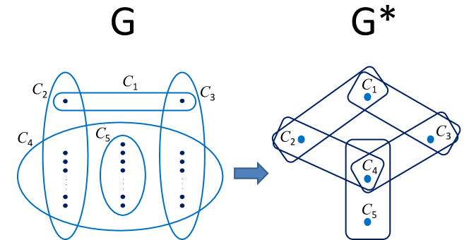
Figure 2: $G$ and $G^{*}$ from Example 12

Note that the dual of the dual of a hypergraph is not necessarily the original hypergraph, since we do not allow multiple identical hyperedges.

Example 13

Consider the dual hypergraph $G^{*}$ defined in Example 12. Taking the dual of this hypergraph yields $G^{**}$, with vertex set $\{h_{1},\ldots,h_{5}\}$ (corresponding to the 5 hyperedges in $G^{*}$) and 5 distinct hyperedges, as shown in Figure 3.

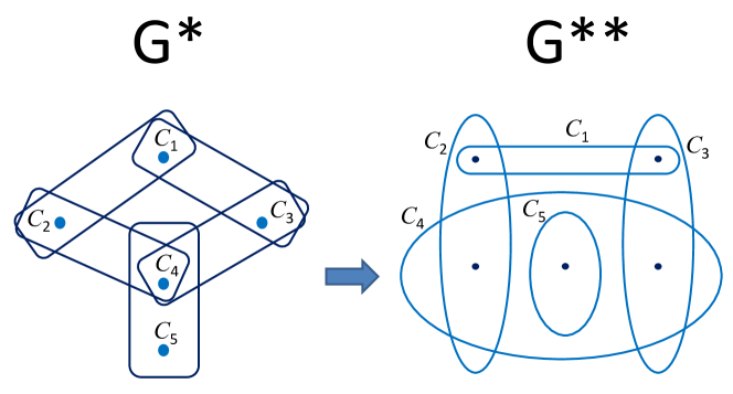
Figure 3: $G^{*}$ and $G^{**}$ from Example 13

In the example above, taking the dual of a hypergraph twice had the effect of merging precisely those sets of variables that occur in the same set of hyperedges. It is easy to verify that this is true in general: Taking the dual twice equates precisely those variables that occur in the same set of hyperedges.

Lemma 1

For any hypergraph $G$, the hypergraph $G^{**}$ has precisely one vertex corresponding to each maximal subset of vertices of $G$ that occur in the same set of hyperedges.

Next, we combine the idea of the dual with the usual notion of treewidth to create a new measure of width.

Definition 18 (twDD)

Let $G$ be a hypergraph. The treewidth of the dual of the dual (twDD) of $G$ is $\mathsf{twDD}(G)=\mathsf{tw}(G^{**})$.

For a class of hypergraphs $\mathcal{H}$, we define $\mathsf{twDD}(\mathcal{H})=\mathsf{tw}(\mathcal{H}^{**})$.

Example 14

Consider the class $\mathcal{H}$ of hypergraphs of the family of problems described in Example 1. Whatever the value of $n$, the dual hypergraph, $G^{*}$ is the same, as shown in Figure 2. Hence for all problems in this family the hypergraph $G^{**}$ is as shown in Figure 3, and can be shown to have treewidth 3. Hence $\mathsf{twDD}(\mathcal{H})=3$.

When replacing a set of variables in a CSP instance with a single variable, we will use the following definition.

Definition 19 (Quotient of a CSP instance)

Let $P=\langle V,C\rangle$ be a CSP instance and $X\subseteq V$ be a non-empty subset of variables that all occur in the scopes of the same set $S$ of constraints. The quotient of $P$ with respect to $X$, denoted $P^{X}$, is defined as follows.

• The variables of $P^{X}$ are given by $V^{X}=(V-X)\cup\{v_{X}\}$, where $v_{X}$ is a fresh variable, and the domain of $v_{X}$ is the set of equivalence classes of $\mathsf{equiv}[\mathsf{join}(S),X]$.

• The constraints of $P^{X}$ are unchanged, except that each constraint $e[\delta]\in S$ is replaced by a new constraint $e^{X}[\delta^{X}]$, where $\mathsf{vars}(\delta^{X})=(\mathsf{vars}(\delta)-X)\cup\{v_{X}\}$. For any assignment $\theta$ of $\mathsf{vars}(\delta^{X})$, we define $e^{X}[\delta^{X}](\theta)$ to be 1 if and only if $\theta|_{\mathsf{vars}(\delta)-X}\oplus\mu\in e[\delta]$, where $\mu$ is a representative of the equivalence class $\theta(v_{X})$.

We note that, by Definition 11, the value of $e^{X}[\delta^{X}]$ specified in Definition 19 is well-defined, that is, it does not depend on the specific representative chosen for the equivalence class $\theta(v_{X})$, since each representative has the same set of possible extensions.

Lemma 2

Let $P=\langle V,C\rangle$ be a CSP instance and $X\subseteq V$ be a non-empty subset of variables that all occur in the scopes of the same set of constraints. The instance $P^{X}$ has a solution if and only if $P$ has a solution.

Proof (Sketch)

Let $P=\langle V,C\rangle$ and $X$ be given, and let $S\subseteq C$ be the set of constraints $e[\delta]$ such that $X\subseteq\mathsf{vars}(\delta)$.

Construct the instance $P^{X}$ as specified in Definition 19. Any solution to $P$ can be converted into a corresponding solution for $P^{X}$, and vice versa. This conversion process just involves replacing the part of the solution assignment that gives values to the variables in the set $X$ with an assignment that gives a suitable value to the new variable $v_{X}$.

Theorem 5.1

Any CSP instance $P$ can be converted to an instance $P^{\prime}$ with $\mathsf{hyp}(P^{\prime})=\mathsf{hyp}(P)^{**}$, such that $P^{\prime}$ has a solution if and only if $P$ does. Moreover, if $P$ is over a cooperating catalogue, this conversion can be done in polynomial time.

Proof

Let $P=\langle V,C\rangle$ be a CSP instance. For each variable $v\in V$ we define $S(v)=\{e[\delta]\in C\mid v\in\mathsf{vars}(\delta)\}$ We then partition the vertices of $P$ into subsets $X_{1},\ldots,X_{k}$, where each $X_{i}$ is a maximal subset of variables $v$ that share the same value for $S(v)$.

We initially set $P_{0}=P$. Then, for each $X_{i}$ in turn, we set $P_{i}=(P_{i-1})^{X}$. Finally we set $P^{\prime}=P_{k}$. By Lemma 1, $\mathsf{hyp}(P^{\prime})=\mathsf{hyp}(P)^{**}$, and by Lemma 2, $P^{\prime}$ has a solution if and only if $P$ has a solution.

Finally, if $P$ is over a cooperating catalogue, then by Definition 14, we can compute the domains of each new variable introduced in polynomial time in the size of each $X_{i}$ and the total size of the constraints. Hence we can compute $P^{\prime}$ in polynomial time.

Using Theorem 5.1, we can immediately get a new tractable CSP class by extending Theorem 3.1.

Theorem 5.2

Let $\mathcal{C}$ be a constraint catalogue and $\mathcal{H}$ a class of hypergraphs. $\mathsf{CSP}(\mathcal{H},\mathcal{C})$ is tractable if $\mathcal{C}$ is a cooperating catalogue and $\mathsf{twDD}(\mathcal{H})<\infty$.

Proof

Let $\mathcal{C}$ be a cooperating catalogue, $\mathcal{H}$ a class of hypergraphs such that $\mathsf{twDD}(\mathcal{H})<\infty$, and $P\in\mathsf{CSP}(\mathcal{H},\mathcal{C})$. Reduce $P$ to a CSP instance $P^{\prime}$ using Theorem 5.1. By Definition 18, since $\mathsf{hyp}(P^{\prime})=\mathsf{hyp}(P)^{**}$, $\mathsf{tw}(\mathsf{hyp}(P^{\prime}))<\infty$, which means that $P^{\prime}$ satisfies the conditions of Theorem 3.1, and hence can be solved in polynomial time.

Recall the family of constraint problems described in Example 1 at the start of this paper. Since the constraints in this problem form a cooperating catalogue (Example 11), and all instances have bounded twDD (Example 14), this family of problems is tractable by Theorem 5.2.

6 Summary and Future Work

We have identified a novel tractable class of constraint problems with global constraints. In fact, our results generalize several previously studied classes of problems [12]. Moreover, this is the first representation-independent tractability result for constraint problems with global constraints.

Our new class is defined by restricting both the nature of the constraints and the way that they interact. As demonstrated in Example 5, instances with a single global constraint may already be -complete [26], so we cannot hope to achieve tractability by structural restrictions alone. In other words, notions such as bounded degree of cyclicity [21] or bounded hypertree width [18] are not sufficient to ensure tractability in the framework of global constraints, where the arity of individual constraints is unbounded. This led us to introduce the notion of a cooperating constraint catalogue, which is sufficiently restricted to ensure that an individual constraint is always tractable.

However, this restriction on the nature of the constraints is still not enough to ensure tractability on any structure: Example 6 demonstrates that not all structures are tractable even with a cooperating constraint catalogue. In fact, a family of problems with acyclic structure (hypertree width one) over a cooperating constraint catalogue can still be NP-complete. This led us to investigate restrictions on the structure that are sufficient to ensure tractability for all instances over a cooperating catalogue. In particular, we have shown that it is sufficient to ensure that the dual of the dual of the hypergraph of the instance has bounded treewidth.

An intriguing open question is whether there are other restrictions on the nature of the constraints or the structure of the instances that are sufficient to ensure tractability in the framework of global constraints. Very little work has been done on this question, apart from the pioneering work of Bulatov and Marx [8], which considered only a single global cardinality constraint, along with arbitrary table constraints, and of Chen and Dalmau [9] on two specific succinct representations. Almost all other previous work on tractable classes has considered only table constraints. This may be one reason why such work has had little practical impact on the design of constraint solvers, which rely heavily on the use of in-built special-purpose global constraints.

We see this paper as a first step in the development of a more robust and applicable theory of tractability for global constraints.

References

- [1] Aschinger, M., Drescher, C., Friedrich, G., Gottlob, G., Jeavons, P., Ryabokon, A., Thorstensen, E.: Optimization methods for the partner units problem. In: Proc. CPAIOR’11. LNCS, vol. 6697, pp. 4–19. Springer (2011)
- [2] Aschinger, M., Drescher, C., Gottlob, G., Jeavons, P., Thorstensen, E.: Structural decomposition methods and what they are good for. In: Schwentick, T., Dürr, C. (eds.) Proc. STACS’11. LIPIcs, vol. 9, pp. 12–28 (2011)
- [3] Beeri, C., Fagin, R., Maier, D., Yannakakis, M.: On the desirability of acyclic database schemes. Journal of the ACM 30, 479–513 (July 1983)
- [4] Beldiceanu, N.: Pruning for the minimum constraint family and for the number of distinct values constraint family. In: Proc. CP’01. LNCS, vol. 2239, pp. 211–224. Springer (2001)
- [5] Bessiere, C., Hebrard, E., Hnich, B., Walsh, T.: The complexity of reasoning with global constraints. Constraints 12(2), 239–259 (2007)
- [6] Bessiere, C., Katsirelos, G., Narodytska, N., Quimper, C.G., Walsh, T.: Decomposition of the NValue constraint. In: Proc. CP’10. LNCS, vol. 6308, pp. 114–128. Springer (2010)
- [7] Bulatov, A., Jeavons, P., Krokhin, A.: Classifying the complexity of constraints using finite algebras. SIAM Journal on Computing 34(3), 720–742 (2005)
- [8] Bulatov, A.A., Marx, D.: The complexity of global cardinality constraints. Logical Methods in Computer Science 6(4:4), 1–27 (2010)
- [9] Chen, H., Grohe, M.: Constraint satisfaction with succinctly specified relations. Journal of Computer and System Sciences 76(8), 847–860 (2010)
- [10] Cohen, D.A., Green, M.J., Houghton, C.: Constraint representations and structural tractability. In: Proc. CP’09. LNCS, vol. 5732, pp. 289–303. Springer (2009)
- [11] Cohen, D.A., Jeavons, P., Gyssens, M.: A unified theory of structural tractability for constraint satisfaction problems. Journal of Computer and System Sciences 74(5), 721–743 (2008)
- [12] Dalmau, V., Kolaitis, P.G., Vardi, M.Y.: Constraint satisfaction, bounded treewidth, and finite-variable logics. In: Proc. CP’02. LNCS, vol. 2470, pp. 223–254. Springer (2002)
- [13] Dechter, R., Pearl, J.: Tree clustering for constraint networks. Artificial Intelligence 38(3), 353–366 (1989)
- [14] Freuder, E.C.: Complexity of k-tree structured constraint satisfaction problems. In: Proc. AAAI, pp. 4–9. AAAI Press / The MIT Press (1990)
- [15] Garey, M.R., Johnson, D.S.: Computers and Intractability: A Guide to the Theory of NP-Completeness. W. H. Freeman (1979)
- [16] Gent, I.P., Jefferson, C., Miguel, I.: MINION: A fast, scalable constraint solver. In: Proc. ECAI’06, pp. 98–102. IOS Press (2006)
- [17] Gottlob, G., Leone, N., Scarcello, F.: A comparison of structural CSP decomposition methods. Artificial Intelligence 124(2), 243–282 (2000)
- [18] Gottlob, G., Leone, N., Scarcello, F.: Hypertree decompositions and tractable queries. Journal of Computer and System Sciences 64(3), 579–627 (2002)
- [19] Green, M.J., Jefferson, C.: Structural tractability of propagated constraints. In: Proc. CP’08. LNCS, vol. 5202, pp. 372–386. Springer (2008)
- [20] Grohe, M.: The complexity of homomorphism and constraint satisfaction problems seen from the other side. Journal of the ACM 54(1), 1–24 (2007)
- [21] Gyssens, M., Jeavons, P.G., Cohen, D.A.: Decomposing constraint satisfaction problems using database techniques. Artificial Intelligence 66(1), 57–89 (1994)
- [22] Hermenier, F., Demassey, S., Lorca, X.: Bin repacking scheduling in virtualized datacenters. In: Proc. CP’11. LNCS, vol. 6876, pp. 27–41. Springer (2011)
- [23] van Hoeve, W.J., Katriel, I.: Global constraints. In: Rossi, F., van Beek, P., Walsh, T. (eds.) Handbook of Constraint Programming, Foundations of Artificial Intelligence, vol. 2, chap. 6, pp. 169–208. Elsevier (2006)
- [24] Kutz, M., Elbassioni, K., Katriel, I., Mahajan, M.: Simultaneous matchings: Hardness and approximation. Journal of Computer and System Sciences 74(5), 884–897 (August 2008)
- [25] Marx, D.: Tractable hypergraph properties for constraint satisfaction and conjunctive queries. In: Proc. STOC’10, pp. 735–744. ACM (2010)
- [26] Quimper, C.G., López-Ortiz, A., van Beek, P., Golynski, A.: Improved algorithms for the global cardinality constraint. In: Proc. CP’04. LNCS, vol. 3258, pp. 542–556. Springer (2004)
- [27] Rosen, K.H., Michaels, J.G., Gross, J.L., Grossman, J.W., Shier, D.R. (eds.): Handbook of Discrete and Combinatorial Mathematics. Discrete Mathematics and Its Applications, CRC Press (2000)
- [28] Rossi, F., van Beek, P., Walsh, T. (eds.): The Handbook of Constraint Programming. Elsevier (2006)
- [29] Samer, M., Szeider, S.: Tractable cases of the extended global cardinality constraint. Constraints 16(1), 1–24 (2011)
- [30] Wallace, M.: Practical applications of constraint programming. Constraints 1, 139–168 (September 1996)
- [31] Wallace, M., Novello, S., Schimpf, J.: ECLiPSe: A platform for constraint logic programming. ICL Systems Journal 12(1), 137–158 (May 1997)