Ionization of hydrogen by neutrino magnetic moment, relativistic muon, and WIMP

Abstract

We studied the ionization of hydrogen by scattering of neutrino magnetic moment, relativistic muon, and weakly-interacting massive particle with a QED-like interaction. Analytic results were obtained and compared with several approximation schemes often used in atomic physics. As current searches for neutrino magnetic moment and dark matter have lowered the detector threshold down to the sub-$\mathrm{keV}$ regime, we tried to deduce from this simple case study the influence of atomic structure on the the cross sections and the applicabilities of various approximations. The general features being found will be useful for cases where practical detector atoms are considered.

I Introduction

The electromagnetic (EM) properties of neutrinos, in particular the magnetic dipole moments, $\mu_{\nu}$, are of fundamental importance not only in particle physics but also astrophysics and cosmology (for reviews, see, e.g., Refs. (Beringer et al., 2012; Broggini et al., 2012)). In the Standard Model with massive neutrinos, a non-vanishing $\mu_{\nu}$ arises as a result of one-loop electroweak radiative correction; for Dirac neutrinos,  it is given by $\mu_{\nu}=3.20\times 10^{-19}\,(\frac{m_{\nu}}{\mathrm{eV}})\,\mu_{\mathrm{B}}$, where the Bohr magneton $\mu_{\mathrm{B}}=e/(2\,m_{e})$ with $e$ and $m_{e}$ being the magnitude of charge and mass of electron.  From the current mass upper limit set on the electron neutrino in the tritium $\beta$ decay (Aseev et al., 2011), $m_{\nu_{e}}<2\,\mathrm{eV}$, one can estimate that $\mu_{\nu_{e}}\lesssim 10^{-18}\,\mu_{\mathrm{B}}$ is indeed very tiny in the Standard Model.

The best direct limits on $\mu_{\nu}$ so far are extracted mostly from neutrino-electron ($\nu e$) scattering: with the reactor antineutrinos, $\mu_{\bar{\nu}_{e}}<2.9\times 10^{-11}\,\mu_{\mathrm{B}}$ by the GEMMA collaboration (Beda et al., 2013) and $\mu_{\bar{\nu}_{e}}<7.4\times 10^{-11}\,\mu_{\mathrm{B}}$ by the TEXONO collaboration (Wong et al., 2007); with the solar neutrinos, $\mu_{\nu_{\odot}}<5.4\times 10^{-11}\,\mu_{\mathrm{B}}$ by the Borexino collaboration (Arpesella et al., 2008). Many stronger, but indirect, limits ranging from $10^{-11}$ to $10^{-13}$ were inferred from astrophysical or cosmological constraints, however, they are subject to model dependence and theoretical uncertainty. Because the current limits, whether direct or indirect, are orders of magnitude away from the Standard Model prediction, it makes the search of $\mu_{\nu}$ a powerful probe of new physics.

The cross section of neutrino scattering off a free electron through the EM interaction with $\mu_{\nu}$ is (Vogel and Engel, 1989)

$$\left.\frac{d\sigma}{dT}\right|_{\mathrm{FE}}=4\,\pi\,\alpha\,\mu_{\nu}^{2}\,(\frac{1}{T}-\frac{1}{E_{\nu}})\,,$$ (1)

where $\alpha$ is the fine structure constant, $E_{\nu}$ the neutrino incident energy, and $T$ the neutrino energy deposition. The $1/T$ feature indicates a way of improving the limit on $\mu_{\nu}$ by lowering the detector threshold of $T$. Currently the thresholds can be as low as a few $\mathrm{keV}$ (e.g., the Germanium semiconductor detectors deployed by both the GEMMA and TEXONO collaborations), and the next-generation detectors are geared up to extend down to the sub-$\mathrm{KeV}$ regime (Wong, 2011; Yue and Wong, 2013). While one expects improved limits from such experimental upgrades, a theoretical issue regarding how the electronic structure of detectors affects the simple free $\nu e$ scattering formula naturally arises, as the associated energy scale is comparable to the atomic scale. Recently there have been discussions about whether atomic structure can possibly enhance an atomic ionization (AI) cross section (Wong et al., 2010; Voloshin, 2010), and the robustness of an free electron approximation in low energy transfer (Kouzakov and Studenikin, 2011; Kouzakov et al., 2011). With experiments keep pushing down the detector threshold, the need for more reliable cross section formulae will certainly grow.

Another type of experiments where AI can be relevant is the search for dark matter (DM), as it shares many similar detection techniques as for $\mu_{\nu}$. Most current search focus on the weakly-interacting massive particles (WIMPs) with masses about $\mathrm{GeV}$ to $\mathrm{TeV}$ scales – favoured for astrophysical reasons – with nuclear recoil in targets being the main observable. Recently the sub-$\mathrm{GeV}$ DM candidates, generically classified as light dark matter (LDM), start to get attention (Essig et al., 2012a), and the associated AI processes in targets can be used to constrain the interaction of LDM candidates with electrons and their masses (Essig et al., 2012b).

Given the importance of understanding the detectors’ response, in particular in low energy regime, our study starts by considering the simplest atom – hydrogen. By treating the electrons as non-relativistic particles and including the one photon exchange together with the Coulomb interaction, the problem is solved analytically with $O(v_{e}^{2})$ and $O(\alpha^{2})$ errors, where $v_{e}$ is the electron velocity. We then compare our result against various widely-used approximation schemes for the AI through $\mu_{\nu}$ or DM scattering, we try to draw useful information about the applicabilities of these approximation schemes under various kinematic conditions. This knowledge serves as a precursor to our currently-ongoing projects with realistic atomic species.

The article is organized as follows: In Sec. II, we lay down the general formalism for AI cross sections through EM interactions. The analytic results for the atomic response functions of hydrogen-like atoms are given explicitly, and approximation schemes including the free electron approximation (FEA), equivalent photon approximation (EPA), longitudinal photon approximation (LPA), and the one of Kouzakov, Studenikin, and Voloshin (KSV) (Kouzakov et al., 2011) are introduced. The case of AI by $\mu_{\nu}$ is studied in Sec. III, with particular attention to the issue whether atomic structure enhances or suppresses the cross sections while scattering occurs at atomic scales. In Sec. IV, the well-known AI process by relativistic muon is re-visited. A detailed account of why EPA works for this case but not for $\mu_{\nu}$ is given. Finally we extend the above formalism to a QED-like gauge model for the DM interaction with normal matter, and study the hydrogenic response under various DM kinematics in Sec. V. A brief summary is in Sec. VI.

II Formalism

Consider the ionization of a hydrogen-like atom $\mathrm{H}$ by a lepton $l$,

$$l+\mathrm{H}\rightarrow l+\mathrm{H}^{+}+e^{-}\,,$$ (2)

through one photon exchange, as shown in Fig. 1. We will treat the electron as a non-relativistic particle and include all its Coulomb interactions in the initial and final states. This problem can be solved analytically. The results will be referred as the “full” ones – in comparison to various approximations to be discussed later on – and have errors on the order of $O(v_{e}^{2},\alpha^{2})$.

The unpolarized differential cross section in the laboratory frame, i.e., the velocity of the incident lepton $\vec{v}_{1}\neq 0$ and the velocity of the atomic target $\vec{v}_{\mathrm{H}}=0$, is expressed as 

$$d\sigma= \dfrac{1}{|\vec{v}_{1}|}\,\dfrac{(4\,\pi\,\alpha)^{2}}{Q^{4}}\,\overline{l}^{\mu\nu}\,\overline{W}_{\mu\nu}\,(2\pi)^{4}\,\delta^{4}(k_{1}+p_{\mathrm{H}}-k_{2}-p_{R}-p_{r})\,\dfrac{d^{3}\vec{k}_{2}}{(2\,\pi)^{3}}\,\dfrac{d^{3}\vec{p}_{R}}{(2\,\pi)^{3}}\,\dfrac{d^{3}\vec{p}_{r}}{(2\,\pi)^{3}}\,,$$ (3)

where the four momenta $k_{1}=(\omega_{1},\vec{k_{1}})$ and $k_{2}=(\omega_{2},\vec{k_{2}})$ are of the initial and final leptons, $p_{\mathrm{H}}=(M_{\mathrm{H}},\vec{0})$ of the initial atom, $p_{R}=(E_{R},\vec{p}_{R})$ and $p_{r}=(E_{r},\vec{p}_{r})$ of the final $\mathrm{H}^{+}+e^{-}$ state in the center-of-mass and relative coordinates, and $q^{\mu}=k_{1}^{\mu}-k_{2}^{\mu}=(T,\vec{q})$ of the virtual photon; respectively; and $Q^{2}=q_{\mu}\,q^{\mu}$. The leptonic tensor

$$\overline{l}^{\mu\nu}\equiv\sum_{s_{2}}\overline{\sum_{s_{1}}}\braket{k_{2},s_{2}}{j_{l}^{\mu}}{k_{1},s_{1}}\,\braket{k_{2},s_{2}}{j_{l}^{\nu}}{k_{1},s_{1}}^{*}\,,$$ (4)

is obtained by a sum of the final spin state $s_{2}$ and an average of the initial spin state $s_{1}$ of the leptonic electromagnetic (EM) current, $j_{l}$, matrix elements; and similarly the atomic tensor

$$\overline{W}^{\mu\nu}\equiv\sum_{m_{j_{f}}}\overline{\sum_{m_{j_{i}}}}\braket{f}{j_{A}^{\mu}}{i}\,\braket{f}{j_{A}^{\nu}}{i}^{*}\,,$$ (5)

involves a sum of the final angular momentum state $m_{j_{f}}$ and an average of the initial angular momentum state $m_{j_{i}}$ of the atomic EM current, $j_{A}$, matrix elements, where $\ket{i}$ and $\ket{f}$ refer to atomic initial and final states, respectively.

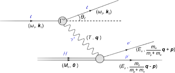
Figure 1: The atomic ionization process $l+\mathrm{H}\rightarrow l+\mathrm{H}^{+}+e^{-}$ through one photon exchange in the laboratory frame.

In this work, we use the relativistic form for $j_{l}^{\mu}$

$$\braket{k_{2},s_{2}}{j_{l}^{\mu}}{k_{1},s_{1}}=\bar{u}(k_{2},s_{2})\,[F_{1}^{(l)}\gamma^{\mu}\,-i\,\frac{F_{2}^{(l)}}{2\,m_{e}}\,\sigma^{\mu\nu}\,q_{\nu}]\,u(k_{1},s_{1})\,.$$ (6)

The Dirac and Pauli form factors, $F_{1}^{(l)}$ and $F_{2}^{(l)}$, which describe the helicity-preserving and helicity-changing EM couplings, are constant for elementary leptons: $F_{1}^{(l)}$ is the charge $e_{l}$ (in units of $e$) and $F_{2}^{(l)}$ the anomalous magnetic dipole moment $\kappa_{l}$ (in units of $\mu_{\mathrm{B}}$) .

Since we are only interested in the case that the energy deposition by the incident particle is small enough such that electrons can be treated as non-relativistic particles, the charge and spatial current densities in momentum space are

$$\rho^{(A)}(\vec{q}) = -\,e^{i\,\,\vec{q}\cdot\left(\vec{R}+\vec{r}\right)}\,,$$ (7)

$$\vec{j}^{(A)}(\vec{q}) = \frac{-1}{2\,m_{e}}\,e^{i\,\,\vec{q}\cdot\left(\vec{R}+\vec{r}\right)}\,(\vec{q}+2\,\vec{p}_{r}+i\,\,\vec{\sigma}_{e}\times\vec{q}).$$ (8)

$\rho^{(A)}$ is leading in the $1/m_{e}$ expansion while $\vec{j}^{(A)}$ is subleading. The proton contribution can be neglected because its contribution to $\vec{j}^{(A)}$ is $O(1/m_{p})$ and is smaller than the electron contribution by a factor of $m_{e}/m_{p}$. Its contribution to $\rho^{(A)}$ is smaller than the electron contribution by at least one power of $m_{e}/m_{p}$ in the multiple expansion, because the size of the proton wave function is smaller than that of the electron wave function by a $m_{e}/m_{p}$ factor.

After performing the spin sum, contraction of the leptonic and atomic tensors, and implementing the current conservation condition to relate the longitudinal spatial current to the charge density

$$j_{\parallel}^{(A)}(\vec{q})\equiv\frac{\vec{q}}{q}\cdot\vec{j}^{(A)}(\vec{q})=\frac{T}{q}\,\rho^{(A)}(\vec{q})\,,$$ (9)

where $q\equiv|\vec{q}|$, the cross section can be cast into the following form

$$d\sigma=\frac{\pi}{|\vec{k}_{1}|}\,\dfrac{(4\,\pi\,\alpha)^{2}}{Q^{4}}\,\sum_{X=L,T}\left[\left(e_{l}^{2}\,V_{X}^{(F_{1})}+\frac{\kappa_{l}^{2}}{(2\,m_{e})^{2}}\,V_{X}^{(F_{2})}\right)\,R_{X}\right]\,\dfrac{d^{3}\vec{k}_{2}}{(2\,\pi)^{3}\,2\,\omega_{2}}\,,$$ (10)

through defining the longitudinal and transverse response functions, $R_{L}$ and $R_{T}$, and the corresponding kinematic factors, $V_{L}$ and $V_{T}$. The kinematic factors, which depend on the energy transfer $T$ and momentum transfer $q$, are

$$V_{L}^{(F_{1})} =\dfrac{Q^{4}}{q^{4}}[(\omega_{1}+\omega_{2})^{2}-q^{2}],$$ (11)

$$V_{T}^{(F_{1})} =-\,\left[\dfrac{Q^{2}(Q^{2}+4\omega_{1}\omega_{2})}{2\,q^{2}}+Q^{2}+2m_{l}^{2}\right]\,,$$ (12)

and

$$V_{L}^{(F_{2})} =\dfrac{-Q^{4}}{q^{4}}\left[(\omega_{1}+\omega_{2})^{2}\,Q^{2}+4\,m_{l}^{2}\,q^{2}\right],$$ (13)

$$V_{T}^{(F_{2})} =\dfrac{Q^{2}}{2\,q^{2}}\left[Q^{2}(Q^{2}+4\,\omega_{1}\,\omega_{2})-4\,m_{l}^{2}\,q^{2}\right]\,,$$ (14)

for couplings with the $F_{1}^{(l)}$ and $F_{2}^{(l)}$ form factors, respectively.  The response functions, which are also functions of $(T,q)$ but independent of the form of leptonic coupling, are

$$R_{L} \equiv \sum_{m_{j_{f}}}\overline{\sum_{m_{j_{i}}}}\int\,\frac{d^{3}\vec{p}_{r}}{(2\,\pi)^{3}}\,|\langle f|\rho^{(A)}(\vec{q})|i\rangle|^{2}\delta\left(T-B-\dfrac{q^{2}}{2M}-\dfrac{p_{r}^{2}}{2\,\mu_{red}}\right)\,,$$ (15)

$$R_{T} \equiv \sum_{m_{j_{f}}}\overline{\sum_{m_{j_{i}}}}\int\,\frac{d^{3}\vec{p}_{r}}{(2\,\pi)^{3}}\,|\langle f|j_{\perp}^{(A)}(\vec{q})|i\rangle|^{2}\delta\left(T-B-\dfrac{q^{2}}{2M}-\dfrac{p_{r}^{2}}{2\,\mu_{red}}\right)\,,$$ (16)

where $B$ is the binding energy of the $\mathrm{H}$ atom, $M=m_{e}+m{}_{p}\approx m_{p}$, and $\mu_{red}=m_{e}\,m_{p}/(m_{e}+m_{p})\approx m_{e}$. Note that the center-of-mass degrees of freedom in the final state have been integrated out by the momentum conservation, which yield $\vec{p}_{R}=\vec{q}$; and the resulting energy conservation delta function properly takes care the nuclear recoil effect.

Consider now the ionization of a hydrogen-like atom from its ground state, i.e., the $1s$ orbit, the relevant atomic spatial wave functions for the initial ($i$) and final ($f$) states are

$$\braket{\vec{r}}{i} = \braket{\vec{r}}{(nlm_{l}=100)}=\frac{1}{\sqrt{\pi}}\,Z^{3/2}\,e^{-Z\,\bar{r}}\,,$$ (17)

$$\braket{f}{\vec{r}} = {}^{(-)}\braket{\vec{p}_{r}}{\vec{r}}=e^{\frac{\pi\,Z}{2\,\bar{p}_{r}}}\Gamma\left(1-\dfrac{i\,Z}{\bar{p}_{r}}\right)\,e^{-i\,\vec{p}_{r}\cdot\vec{r}}{{}_{1}F_{1}}\left(\dfrac{i\,Z}{\bar{p}_{r}},1,i(p_{r}\,r+\vec{p}_{r}\cdot\vec{r})\right)\,,$$ (18)

in atomic units (so the barred quantities are $\bar{r}=r\,m_{e}\,\alpha$, $\bar{p}_{r}=p/(m_{e}\,\alpha)$, etc.), where $\Gamma(z)$ and ${{}_{1}F_{1}}(a,b,z)$ are the Gamma and confluent hypergeometric functions, respectively. The evaluations of $R_{L}$ and $R_{T}$ can be done analytically by the Nordsieck integration (Nordsieck, 1954; Holt, 1969; Belkić, 1981; Gravielle and Miraglia, 1992) and yield:

$$R_{L} =\frac{2^{8}\,Z^{6}\,\bar{q}^{2}\,(3\,\bar{q}^{2}+\bar{p}_{r}^{2}+Z^{2})\,\exp\left[-\frac{2\,Z}{\bar{p}_{r}}\tan^{-1}\left(\frac{2\,Z\,\bar{p}_{r}}{\bar{q}^{2}-\bar{p}_{r}^{2}+Z^{2}}\right)\right]}{3\,((\bar{q}+\bar{p}_{r})^{2}+Z^{2})^{3}\,((\bar{q}-\bar{p}_{r})^{2}+Z^{2})^{3}\,(1-e^{-2\,\pi\,Z/\bar{p}_{r}})}$$ (19)

$$R_{T} =\frac{2^{7}\,\alpha^{2}\,Z^{6}\,(\bar{p}_{r}^{2}+Z^{2})\,\exp\left[-\frac{2\,Z}{\bar{p}_{r}}\tan^{-1}\left(\frac{2\,Z\,\bar{p}_{r}}{\bar{q}^{2}-\bar{p}_{r}^{2}+Z^{2}}\right)\right]}{3\,((\bar{q}+\bar{p}_{r})^{2}+Z^{2})^{2}\,((\bar{q}-\bar{p}_{r})^{2}+Z^{2})^{2}\,(1-e^{-2\,\pi\,Z/\bar{p}_{r}})}+\frac{1}{2}\,\mu_{e}^{2}\,\alpha^{2}\,\bar{q}^{2}\,R_{L}\,.$$ (20)

The first term in $R_{T}$ is the contribution from the convection current, and the second one from the spin current. The overall $\alpha^{2}$ factor appearing in both terms reflects the $1/m_{e}^{2}$ order in the non-relativistic expansion. In comparison, $R_{L}$ is $O(\alpha^{0})$.

The single differential cross section with respect to the energy transfer can then be computed by integration over the lepton scattering angle $\theta$

$$\dfrac{d\sigma}{dT} =\int\,d\cos\theta\,\dfrac{2\,\pi\,\alpha^{2}}{Q^{4}}\dfrac{k_{2}}{k_{1}}\left(V_{L}\,R_{L}+V_{T}\,R_{T}\right)$$ (21)

$$V_{L,T} =e_{l}^{2}\,V_{L,T}^{(F_{1})}+\frac{\kappa_{l}^{2}}{(2\,m_{e})^{2}}\,V_{L,T}^{(F_{2})}$$

with a constrained range of $\cos\theta$:

$$\min\left\{1,\max\left[-1,\dfrac{k_{1}^{2}+k_{2}^{2}-2\,M_{H}\,(T-B)}{2\,k_{1}\,k_{2}}\right]\right\}\leq\cos\theta\leq 1.$$ (22)

For latter discussion, we note that for a fixed energy transfer, the square of four momentum transfer:

$$Q^{2}=2\,m_{l}^{2}-2\,\omega_{1}\,(\omega_{1}-T)+2\,\sqrt{\omega_{1}^{2}-m_{l}^{2}}\,\sqrt{(\omega_{1}-T)^{2}-m_{l}^{2}}\,\cos\theta\,,$$ (23)

only depends on $\cos\theta$, therefore, the integration over $\cos\theta$ is equivalent of integrating over $Q^{2}$ (or $q^{2}$).

While it is straightforward to obtain complete and analytic results for ionizations of the hydrogen atom to the order outlined above,  we shall discuss several approximation schemes often employed in atomic calculations, and compare them with the full calculations for this case study in the following sections.

II.1 Free Electron Approximation (FEA)

The FEA is expected be a good approximation if the photon wavelength is much smaller than the size of the atom (or the typical distance between electrons in a multi-electron system) such that the atomic effect is no longer important. Thus, a necessary (but not sufficient) condition for this approximation to be valid is that the scattering energy needs to be high (compared with the typical scale of the problem).

In this approximation, the electron before and after ionization is treated as a free particle. The free electron cross section of Eq.(1) is multiplied by the step function $\theta(T-B)$ to incorporate the binding effect:

$$\left.\dfrac{d\sigma}{dT}\right|_{FEA}=\theta(T-B)\left.\dfrac{d\sigma}{dT}\right|_{FE}\,.$$ (24)

Energy and momentum conservation fixes $Q^{2}=-2\,m_{e}\,T$ in this two-body phase space.

II.2 Equivalent Photon Approximation (EPA)

The equivalent photon approximation (von Weizsacker, 1934; Williams, 1934) treats the virtual photon as a real (and thus transversely polarized) photon. It could be a good approximation for low energy processes where the photon is soft such that $Q^{2}\approx 0$ because $q^{\mu}\approx 0$ for every component of $\mu$. At high energies, besides soft photon emissions, when the initial and final state electrons are highly relativistic and almost collinear, the emitted “collinear” photon also has $Q^{2}\approx 0$. While the soft photon emission is likely to dominate the phase space of low energy scattering, whether the soft and collinear photon emission will dominate the high energy scattering depends on the transition matrix elements.

The total cross section $\sigma_{\gamma}$ for the photoionization process $\gamma+\mathrm{H}\rightarrow\mathrm{H}^{+}+e^{-}$ is

$$\sigma_{\gamma}(T)=\dfrac{2\,\pi^{2}\,\alpha}{T}\,R_{T}^{0}\,,$$ (25)

where the photon energy $E_{\gamma}=T$ and the superscript “$0$” denotes that the photon is “on-shell”, i.e., $T^{2}=q^{2}$. Then EPA relates $\sigma_{\gamma}$ to a corresponding lepto-ionization process (involving a virtual photon) by the following two steps: (i) ignoring the longitudinal response function $R_{L}$ and (ii) substituting the off-shell response function $R_{T}$ by the on-shell $R_{T}^{0}$ extracted from the photo-ionization process, i.e.,

$$\left.\dfrac{d\sigma}{dT}\right|_{\mathrm{EPA}} =\int\,d\cos\theta\,\dfrac{2\,\pi\,\alpha^{2}}{Q^{4}}\dfrac{k_{2}}{k_{1}}\left[V_{T}\left(\dfrac{T}{2\,\pi^{2}\,\alpha}\,\sigma_{\gamma}(T)\right)\right]\,,$$

$$\equiv\frac{1}{T}\,N(T)\,\sigma_{\gamma}(T)\,,$$ (26)

with the energy spectrum of equivalent photon $N(T)$ defined by

$$N(T)=\frac{\alpha}{\pi}\,\frac{k_{2}}{k_{1}}\,T^{2}\,\int\,d\cos\theta\,\frac{V_{T}}{Q^{4}}\,,$$ (27)

where the integration range of $\cos\theta$ is the same as Eq. (22). Because it directly feeds the photo-ionization cross sections (experimental accessible) to the corresponding lepto-ionization cross sections, a lot of theoretical work and uncertainties can be saved when it works properly.

At this point, we should make an important remark as regards the approximation scheme adopted in Ref. (Wong et al., 2010): Even though it is in the spirit of the EPA, however, it makes a stronger assumption that the integration leading to energy spectrum of equivalent photon is also dominated by the $Q^{2}\approx 0$ region (or staying constant), i.e.,

$$\left.N(T)\right|_{\mathrm{EPA^{\ast}}}\approx\frac{\alpha}{\pi}\,\frac{k_{2}}{k_{1}}\,T^{2}\,\int\,d\cos\theta\,\left.\frac{V_{T}}{Q^{4}}\right|_{Q^{2}\approx 0}\,.$$ (28)

To distinguish this stronger version of the EPA from the conventional one, we shall denote it as the EPA^∗ scheme.

II.3 Longitudinal Photon Approximation (LPA)

The longitudinal photon contribution is leading order in the $1/m_{e}$ expansion while the transverse photon contribution is subleading. Thus, it might be a good approximation for non-relativistic systems:

$$\left.\dfrac{d\sigma}{dT}\right|_{\mathrm{LPA}}=\int\,d\cos\theta\,\dfrac{2\,\pi\,\alpha^{2}}{Q^{4}}\,\dfrac{k_{2}}{k_{1}}\,V_{L}\,R_{L}\,.$$ (29)

The difference of this approximation to the full calculation is a measure of how importantly the transverse current contributes to the process.

II.4 Approximation Scheme of Kouzakov, Studenikin, and Voloshin (KSV)

The KSV scheme includes the longitudinal photon contribution which is leading order in the $1/m_{e}$ expansion and approximates the subleading transverse photon contribution by a relation only strictly suitable for the electric dipole ($E_{1}$) transition in the long wavelength limit, i.e., $q\rightarrow 0$:

$$R_{T}=2\,\frac{T^{2}}{q^{2}}\,R_{L}\,.\,$$ (30)

This relation can be derived from the Siegert theorem (Siegert, 1937) for $E_{1}$, which is based on current conservation. It can also be explicitly checked by taking the same limit to Eqs. (19,20). In general $R_{T}$ is not dominated by $E_{1}$ in the processes that we are considering, which requires $q\,r_{A}\ll 1$ where $\,r_{A}$ is the size of the atom. But Eq. 30 can still be a good approximation to the cross section calculations as long as $R_{T}$ remains subleading to $R_{L}$.

In Refs. (Kouzakov and Studenikin, 2011; Kouzakov et al., 2011), the authors adopted the above relation so the cross section were calculated without need to evaluate the transverse response function which is harder to compute:

$$\left.\dfrac{d\sigma}{dT}\right|_{\mathrm{KSV}}=\int\,d\cos\theta\,\dfrac{2\,\pi\,\alpha^{2}}{Q^{4}}\dfrac{k_{2}}{k_{1}}\left(V_{L}+2\,\frac{T^{2}}{q^{2}}\,V_{T}\right)R_{L}\,.$$ (31)

III Ionization by Neutrino Magnetic Moment

In case the incident lepton is a neutrino ($\nu$) or antineutrino ($\bar{\nu}$), as $e_{\nu}=0$, the EM breakup process is thus sensitive to the neutrino magnetic moment $\mu_{\nu}=\kappa_{\nu}\,\mu_{\mathrm{B}}$ (which is purely anomalous). The energy spectrum for reactor antineutrinos typically peaks around few tens of $\mathrm{keV}$ to $\mathrm{MeV}$ (see, e.g., Ref. (Wong et al., 2007)); setting $\omega_{1}=1\,\mathrm{MeV}$, a plot of the single differential cross section with energy loss up to $1\,\mathrm{keV}$ is given in Fig. 2. Not shown in these figures are the results of the approximation schemes KSV and LPA. They both agree with the full calculation to good extents: within $10^{-5}$ for the former and $10^{-3}$ for the latter in the entire range. In other words, this atomic bound-to-free transition is dominated by the atomic charge operator, while the transverse current operator is negligible, which implies the inadequacy of the EPA scheme.

The dominance of the charge operator over the transverse current can be roughly understood by a comparison of their corresponding kinematic factors $V_{L}^{(F_{2})}$ and $V_{T}^{(F_{2})}$. For neutrino scattering

$$Q^{2}|_{m_{\nu=0}}\approx-2\,\omega_{1}^{2}(1-x)\,,$$ (32)

where $x\equiv\cos\theta$, they are

$$\frac{V_{L}^{(F_{2})}}{Q^{4}}=\frac{2\,(1-x)}{(1-x+\frac{T^{2}}{2\,\omega_{1}^{2}})^{2}}\,, \qquad\frac{V_{T}^{(F_{2})}}{Q^{4}}=\frac{(1+x)}{2\,(1-x+\frac{T^{2}}{2\,\omega_{1}^{2}})}\,.$$ (33)

As $T^{2}/\omega_{1}^{2}\ll 1$ in our consideration, both functions peak near $x=1$, and they have similar maximum values: $V_{L}^{(F_{2})}/Q^{4}|_{\mathrm{max}}=\omega_{1}^{2}/T^{2}$ and $V_{T}^{(F_{2})}/Q^{4}|_{\mathrm{max}}=2\,\omega_{1}^{2}/T^{2}$, and widths. Since the transverse response function does not get enhancement from the kinematic factor $V_{T}^{(F_{2})}$ over $V_{L}^{(F_{2})}$, its contribution to the cross section is suppressed by the usual non-relativistic order $\alpha^{2}$.

(a) $\omega_{1}=1\,\mathrm{MeV}$

(b) $\omega_{1}=1\,\mathrm{MeV}$, near threshold $T$

Figure 2: Differential cross sections $\frac{d\sigma}{dT}$ for $\bar{\nu}+\mathrm{H}\rightarrow\bar{v}+p+e^{-}$ via the EM interaction with the neutrino magnetic moment $\mu_{\nu}=\kappa_{\nu}\,\mu_{\mathrm{B}}$. The incident neutrino has energy $\omega_{1}=1\,\mathrm{MeV}$ with its mass $m_{\nu}$ taken to be zero. The results of the approximation schemes KSV and LPA (both not shown) are in excellent agreement with the full calculation.

The good agreements with the FEA scheme (Fig. 2a) is not really a surprise: the energetic neutrino emits a virtual photon with wavelength smaller than the atomic size so that the binding effect does not manifest in a short distance. The only exception is near the ionization threshold (Fig. 2b) where the virtual photon wavelength is larger than the atomic size, and the binding effect suppresses the cross section in comparison to FEA.

Also shown in these figures is the result of the EPA^∗ scheme. Note that the curve in Fig. 2a has to be scaled down by a factor of $100$ in order to be cast on the same plot as other calculations; in other words, the EPA^∗ hugely overestimates the cross section by several orders of magnitude. There is only a tiny region near the ionization threshold (see Fig. 2b) where the EPA^∗ does work; that is where the virtual photon approaches the real photon limit ($T=q$). The origin of such an overestimate can be clearly seen in Fig. 3a, where the double differential cross section $d\sigma/(dT\,dx)$ is plotted as a function of $x$ with a fixed energy loss $T=20\,\mathrm{eV}$. Due to the kinematic constraint, the maximum scattering angle $\theta_{max}=6.28^{\circ}$. However, even within this small range of peripheral scattering angle, the differential cross section decreases dramatically by $12$ orders of magnitude from the forward angle as a combined result of the kinematic factors $V_{L,T}$ and the response functions $R_{L,T}$. Therefore, the flatness of $d\sigma/(dT\,dx)$ required by the EPA^∗ is severely violated and results in this overestimation.

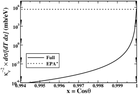
(a) $\omega_{1}=1\,\mathrm{MeV}$, $T=20\,\mathrm{eV}$

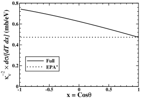
(b) $\omega_{1}=1\,\mathrm{keV}$, $T=20\,\mathrm{eV}$

Figure 3: Double differential cross sections $\frac{d\sigma}{dT\,d\cos\theta}$ for $\bar{\nu}+\mathrm{H}\rightarrow\bar{v}+p+e^{-}$ via the EM interaction with the neutrino magnetic moment $\mu_{\nu}$. The energy transfer is fixed at $20\,\mathrm{eV}$. EPA^∗ hugely overestimates at high $\omega_{1}$, but works reasonably at low $\omega_{1}$.

On the other hand, one does see the EPA^∗ start to work when the incident neutrino energy $\omega_{1}$ drops below the binding momentum of the hydrogen-like atom $\sim Z\,m_{e}\,\alpha$. For hydrogen, the scale is about $3.73\,\mathrm{keV}$, and Fig. 4 shows that varying $\omega_{1}$ from $3\,\mathrm{keV}$, $2\,\mathrm{keV}$, to $1\,\mathrm{keV}$, the EPA^∗ result becomes reasonably good. As evidenced from Fig. 3b, the double differential cross section for $\omega_{1}=1\,\mathrm{keV}$ and $T=20\,\mathrm{eV}$, even though not looking completely flat, does vary only modestly with increasing $\theta$, and the agreement is getting better when $\omega_{1}$ is further decreased. In the meanwhile, the FEA is no longer a good approximation since the de Broglie wavelength of the incident neutrino is on the order of atomic size so the binding effect is not negligible.

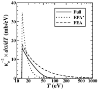
(a) $\omega_{1}=3\,\mathrm{keV}$

(b) $\omega_{1}=2\,\mathrm{keV}$

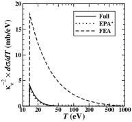
(c) $\omega_{1}=1\,\mathrm{keV}$

Figure 4: Differential cross sections $\frac{d\sigma}{dT}$ for $\bar{\nu}+\mathrm{H}\rightarrow\bar{v}+p+e^{-}$ via the EM interaction with the neutrino magnetic moment $\mu_{\nu}$ at few $\mathrm{keV}$ incident energies. The EPA^∗ calculations gradually converge to the full ones.

IV Ionization by Muon

Replacing the incident lepton from a neutrino to a muon $(\mu^{-})$, as $e_{\mu^{-}}=-1$, the EM breakup process is instead dominated by the $F_{1}$ coupling, while the $F_{2}$ coupling can be ignored for the smallness of muon $g-2\approx 0.001$ (Beringer et al., 2012). Consider relativistic muons with $10^{0,1,2,3}\,\mathrm{GeV}$ energies, the differential cross sections are plotted in Fig. 5. (Because the muon is relativistic while the electron non-relativistic, the final state interaction between the muon and electron can be ignored, see, e.g., Ref. (Landau and Lifshitz, 1981).) The noticeable differences in comparison to what have been drawn in the previous neutrino case are: (1) The differential cross section falls off more quickly as $T$ increases, i.e., the recoil electrons tend to have relatively smaller energies. (2) The FEA results are insensitive to $\omega_{1}$ and largely underestimates in all cases. (3) There are substantial contributions from the transverse current, despite its built-in $O(Z^{2}\,\alpha^{2})$ suppression due to the non-relativistic kinematics of atomic electrons. In fact, when $\omega_{1}$ becomes big enough, the interaction with the atomic transverse current dominates over the one with the charge and longitudinal current, as indicated by the competition between the EPA and the LPA curves in Fig. 5, and one expects the larger $\omega_{1}$ increases, the better the EPA works.

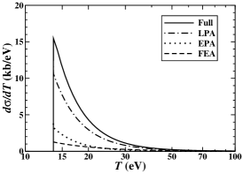
(a) $\omega_{1}=1\,\mathrm{GeV}$

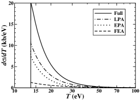
(b) $\omega_{1}=10\,\mathrm{GeV}$

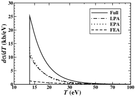
(c) $\omega_{1}=100\,\mathrm{GeV}$

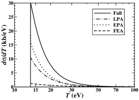
(d) $\omega_{1}=1000\,\mathrm{GeV}$

Figure 5: Differential cross sections $\frac{d\sigma}{dT}$ for $\mu^{-}+\mathrm{H}\rightarrow\mu^{-}+p+e^{-}$ via the EM interaction. The results of the approximation schemes KSV (not shown) are in excellent agreement with the full calculation.

The reason for such differences is primarily due to the associated kinematic factors. At the $Q^{2}\rightarrow 0$ limit, they behave like $V_{L}^{(F_{1})}\propto Q^{4}$ and $V_{T}^{(F_{1})}\propto Q^{0}$ for muon ($m_{\mu}\neq 0$), and $V_{L}^{(F_{2})}\propto Q^{6}$ and $V_{T}^{(F2)}\propto Q^{4}$ for neutrino ($m_{\nu}\approx 0$) ionization, respectively. As the differential cross section $d\sigma/dT$ involves an $1/Q^{4}$ weighted integration over $Q^{2}$, only the transverse part in muon ionization receives a strong weight at peripheral scattering angles (where $Q^{2}\approx 0$).This explains the importance of the transverse current in relativistic muon ionization and its insignificance in neutrino ionization. Also, with the allowed scattering angles become closer to the exact forward direction as the muon incident energy increases (with $T$ fixed), the kinematics becomes real-photon-like and eventually the huge enhancement by the $1/Q^{4}$ weight is able to overcome the non-relativistic suppression in the transverse response function. The failure of the FEA in relativistic muon ionization can also be understood in a similar way: In the FEA scheme, the differential cross section $d\sigma/dT$ is determined from a specific kinematics $Q_{\mathrm{FEA}}^{2}=-2\,m_{e}\,T$ by energy-momentum conservation; on the other hand, the full calculation with two-body kinematics involves an integration over allowed $|Q^{2}|$ ranging from $\approx 0$ to some maximum value determined by the maximum scattering angle. Because the $1/Q^{4}$ factor that enhances the contributions from the $Q^{2}\approx 0$ region, the $Q_{\mathrm{FEA}}^{2}=-2\,m_{e}\,T$ ceases to be a good representative point.

A semi-quantitative understanding could be obtained by the following approximate forms of $V_{L}^{(F_{1})}$ and $V_{T}^{(F_{1})}$. For a relativistic muon

$$Q^{2}|_{\omega_{1}\gg m_{\mu}}\approx-2\,\omega_{1}^{2}\,(1-x)-m_{\mu}^{2}\,\frac{T^{2}}{\omega_{1}^{2}}\,,$$ (34)

they are

$$\frac{V_{L}^{(F_{1})}}{Q^{4}} =\frac{1}{2\,\omega_{1}^{2}}\,\frac{(1+x)}{(1-x+\frac{T^{2}}{2\,\omega_{1}^{2}})^{2}}\,,$$

$$\frac{V_{T}^{(F_{1})}}{Q^{4}} =\frac{1}{4\,\omega_{1}^{2}}\,\frac{(1-x)(3-x)+(3+x)\,\frac{m_{\mu}^{2}}{\omega_{1}^{2}}\,\frac{T^{2}}{2\,\omega_{1}^{2}}}{(1-x+\frac{T^{2}}{2\,\omega_{1}^{2}})(1-x+\frac{m_{\mu}^{2}}{\omega_{1}^{2}}\,\frac{T^{2}}{2\,\omega_{1}^{2}})^{2}}\,.$$ (35)

One sees that unlike the previous case for which $V_{T}^{(F_{2})}$ and $V_{L}^{(F_{2})}$ are comparable in most range of $x$, $V_{T}^{(F_{1})}/Q^{4}$ is comparable to $V_{L}^{(F_{1})}/Q^{4}$ only for $1-x\gtrsim\frac{T^{2}}{2\,\omega_{1}^{2}}$. As the scattering angle further decreases, $V_{T}^{(F_{1})}/Q^{4}$ starts to dominate over $V_{L}^{(F_{1})}/Q^{4}$, and when $1-x\lesssim\frac{m_{\mu}^{2}}{\omega_{1}^{2}}\,\frac{T^{2}}{2\,\omega_{1}^{2}}$, it overwhelms by a factor $\frac{\omega_{1}^{2}}{m_{\mu}^{2}}\gg 1$. Also because of this huge weight on extremely small angles, the FEA scheme with $|Q_{\mathrm{FEA}}^{2}|=2\,m_{e}\,T$ overestimates the averaged $\overline{|Q^{2}|}$ for the realistic situation and leads to an underestimation.

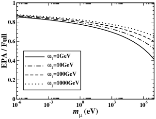
Figure 6: The EPA scheme as an approximation for the relativistic muon ionization with an adjustable $m_{\mu}$, with $T=15\,\mathrm{eV}$.

Though one sees that the EPA serves as a better approximation than the FEA in the relativistic muon ionization, however, as shown in Fig. 5, even at $\omega_{1}=1000\,\mathrm{GeV}$, it can still not be taken as a good approximation to the full result. The main reason is its non-zero mass which limits the lowest |$Q^{2}|$ to be reached

$$|Q^{2}|_{\min}\approx\frac{T^{2}}{\omega_{1}^{2}}\,m_{\mu}^{2}|_{\omega_{1}\gg m_{\mu}\gg T}\,.$$ (36)

If $m_{\mu}$ is adjusted to smaller values $\lesssim 1\,\mathrm{eV}$, then indeed the EPA accounts for $\gtrsim 80\%$ of the cross section for $\omega_{1}$ on the orders of $\mathrm{GeV}-\mathrm{TeV}$, as shown in Fig. 6. In other words, in case one seeks a better description of relativistic muon ionization or other processes alike beyond the EPA, the contribution from charge and longitudinal current should be included.

V Ionization by WIMP

Instead of a relativistic muon, consider now the atomic ionization by some non-relativistic, weakly interacting massive particle, $\chi$, which could be a dark matter (DM) candidate. Suppose this particle is of galactic origin with a mean velocity $v_{\chi}\sim 220/(3\times 10^{5})$, its kinetic energy $\approx\frac{1}{2}\,m_{\chi}\,v_{\chi}^{2}=270\,(\frac{m_{\chi}}{\mathrm{GeV}})\,\mathrm{eV}$; therefore, in order to ionize a hydrogen, $m_{\chi}\gtrsim 60\,\mathrm{MeV}$. To make use of the general formalism developed in Sec. II, we postulate a QED-like fermionic DM-electron ($\chi e$) interaction in which the new $U(1)$ gauge boson has mass $m_{b}$ and the interaction strength $\alpha_{\chi e}\equiv g_{\chi e}\,\alpha$. Fig. 7 shows the differential cross sections for $m_{\chi}=100\,\mathrm{MeV}$ and $1\,\mathrm{GeV}$, with either a massless gauge boson $m_{b}=0$, which corresponds to an infinitely-ranged interaction, or a very massive one $m_{b}=125\,\mathrm{GeV}$, which leads to a extremely short-ranged interaction. 

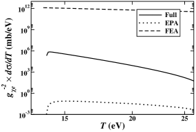
(a) $m_{\chi}=0.1\,\mathrm{GeV}$, $m_{b}=0$

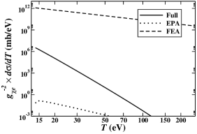
(b) $m_{\chi}=1\,\mathrm{GeV}$, $m_{b}=0$

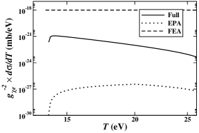
(c) $m_{\chi}=0.1\,\mathrm{GeV}$, $m_{b}=125\,\mathrm{GeV}$

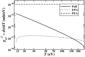
(d) $m_{\chi}=1\,\mathrm{GeV}$, $m_{b}=125\,\mathrm{GeV}$

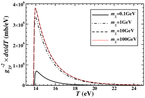
(e) $m_{b}=0$, near threshold

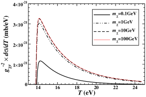
(f) $m_{b}=125\,\mathrm{GeV}$, near threshold

Figure 7: Differential cross sections $d\sigma/dT$ for $\chi+\mathrm{H}\rightarrow\chi+p+e^{-}$ via a QED-like $\chi$–$e$ interaction with the $U(1)$ gauge boson of mass $m_{b}$ and interaction strength $g_{\chi e}\,\alpha$. The results of the approximation schemes KSV and LPA (not shown in (a)–(d)) are in excellent agreement with the full calculation, and only the full resutls are shown in (e) and (f).

Not shown in Fig. 7(a)–(d) are the results of the KSV and LPA, as they are in excellent agreement with the full calculations in all cases illustrated. Accordingly, the failure of the EPA scheme is anticipated. On the other hand, although it is expected that the binding effect should suppress the FEA results, the several orders of magnitude overestimation by the FEA scheme in the entire range of energy transfer, evidenced in panels (a)–(d), indicates the inadequacy of the FEA scheme in such a kinematic regime. Figs. 7(e) and (f) show that the differential cross section becomes “saturated” when $m_{\chi}$ becomes much bigger than $1\,\mathrm{GeV}$, which is about the mass of the hydrogen target. This can be understood by transforming the laboratory frame, where the hydrogen target is stationary, to the DM rest frame which coincides the center-of-mass frame for $m_{\chi}\gg m_{p}$: the kinematics only depends on $v_{\chi}$ and the reduced mass $\approx m_{p}$. Also by comparing the case with $m_{b}=0$, Figs. 7(a,b,e), and $m_{b}=125\,\mathrm{GeV}$, Figs. 7(b,d,e), the differential cross sections, apart from some overall scale factors, show a slower decreasing with energy transfer $T$ as the range of the $\chi e$ interaction decreases.

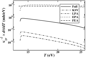
(a) $m_{\chi}=0.1\,\mathrm{GeV}$, $m_{b}=0$

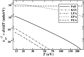
(b) $m_{\chi}=1\,\mathrm{GeV}$, $m_{b}=0$

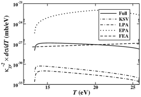
(c) $m_{\chi}=0.1\,\mathrm{GeV}$, $m_{b}=125\,\mathrm{GeV}$

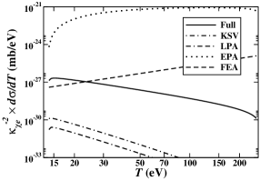
(d) $m_{\chi}=1\,\mathrm{GeV}$, $m_{b}=125\,\mathrm{GeV}$

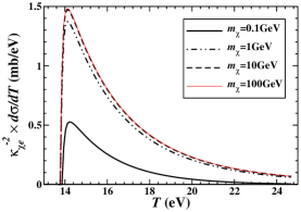
(e) $m_{b}=0$, near threshold

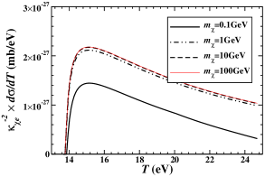
(f) $m_{b}=125\,\mathrm{GeV}$, near threshold

Figure 8: Differential cross sections $d\sigma/dT$ for $\chi+\mathrm{H}\rightarrow\bar{v}+p+e^{-}$ via an anomalous-magnetic-moment-like $\chi$–$e$ interaction with the $U(1)$ gauge boson of mass $m_{b}$ and coupling strength $\kappa_{\chi e}\,\alpha$. Only the full results are shown in (e) and (f).

If, on other hand, the neutral fermionic dark matter has a non-zero (anomalous) magnetic moment, or its coupling to the $U(1)$ gauge boson is via the Dirac bilinear $\bar{\chi}\,\sigma_{\mu\nu}\,q^{\nu}\,\chi/(2\,m_{e})$, a different constant $\alpha_{\chi e}=\kappa_{\chi e}\,\alpha$ is assigned to characterize the interaction strength. This anomalous-magnetic-moment-like interaction yields quite different results, as shown in Fig. 8, from the previous case with the same kinematics. The most noticeable difference seen in Figs. 8(a)–(d) is that the KSV and LPA no longer work, and in fact, largely underestimate. This implies not only substantial contributions from the transverse response but also the breakdown of long wavelength approximation, which has been good for all cases previously discussed. However, the EPA does not work either: it yields a huge overestimate which implies the transverse kinematics is not dominated by the photon-like, $Q^{2}\approx 0$, region. Therefore, one encounters a very subtle kinematic regime where none of the approximation schemes work and requires a full calculation. While Figs. 8(e) and (f) show a similar cross section saturation for $m_{\chi}\gg m_{p}$ and the range effect on the differential cross section as previously found, a comparison of Fig. 8 and Fig. 7 shows that the large energy transfer regime is more suppressed in the QED-like interaction than the anomalous-magnetic-moment-like interaction.

The general trend observed above for the $\chi e$ cross sections that the atomic charge operator dominates in the QED-like interaction while the transverse current operator in the anomalous-magnetic-moment-like interaction is opposite to what have been concluded for the ionizations by relativistic muons ($F_{1}$ coupling) and neutrinos ($F_{2}$ coupling). This difference is also partially due to the corresponding kinematic factors: With $m_{\chi}^{2}\gg|Q^{2}|,q^{2},T^{2}$, they are

$$V_{L}^{(F_{1})}\approx 4\,m_{\chi}^{2}\,\frac{Q^{4}}{q^{4}}\,,\qquad V_{T}^{(F_{1})}\approx 2\,m_{\chi}^{2}\,(\frac{|Q^{2}|}{2\,m_{\chi}^{2}}-\frac{T^{2}}{q^{2}})\,;$$ (37)

and

$$V_{L}^{(F_{2})}\approx 4\,m_{\chi}^{2}\,\frac{Q^{4}}{q^{4}}\,(\frac{\omega_{1}\,T}{m_{\chi}^{2}}\,|Q^{2}|-T^{2})\,,\qquad V_{T}^{(F_{2})}\approx 2\,m_{\chi}^{2}\,|Q^{2}|\,(1+\frac{|Q^{2}|}{q^{2}})\,.$$ (38)

The square of four momentum transfer in DM scattering is

$$Q^{2}\approx-(2-r_{E}-2\,\sqrt{1-r_{E}}\,x)\,m_{\chi}^{2}\,v_{\chi}^{2}\,,$$ (39)

where $r_{E}$ is the fraction of the DM kinetic energy transfer to the atom, i.e., $2\,T/(m_{\chi}\,v_{\chi}^{2})$. For most range of $x$ (which is less restricted unless $m_{\chi}\gg m_{p}$) and $r_{E}$ (which can never be zero for ionization), one can estimate $|Q^{2}|\sim m_{\chi}^{2}\,v_{\chi}^{2}$. Because $T^{2}=(r^{2}\,v_{\chi}^{2}/4)\,m_{\chi}^{2}\,v_{\chi}^{2}$, $q^{2}=T^{2}+|Q^{2}|\sim m_{\chi}^{2}\,v_{\chi}^{2}$. Using these estimates, the leading orders in $v_{\chi}$ are $O(1)$ for $V_{L}^{(F_{1})}$, $O(v_{\chi}^{2})$ for $V_{L}^{(F_{1})}$; and $O(v_{\chi}^{4})$ for $V_{L}^{(F_{2})}$, $O(v_{\chi}^{2})$ for $V_{T}^{(F_{2})}$, respectively. Therefore, in ratio to the charge operator, the transverse current is suppressed by $O(v_{\chi}^{2})/O(1)$ in the $F_{1}$-type coupling, while it is enhanced by $O(v_{\chi}^{2})/O(v_{\chi}^{4})$ in the $F_{2}$-type coupling due to the kinematic factors.

VI Conclusion

We studied the ionization of hydrogen by scattering of neutrino magnetic moment, relativistic muon, and weakly-interacting massive particle with a QED-like interaction. Analytic results were obtained and compared with several approximation schemes often used in atomic physics. It is found that for the case of neutrino magnetic moment, the atomic charge operator dominates the process, and for typical reactor neutrino energies about tens of $\mathrm{keV}$ to a few $\mathrm{MeV}$, the atomic binding effect is negligible. For relativistic muon scattering, on the other hand, the transverse current operator becomes dominant with increasing incident muon energy. In this case, the equivalent photon approximation yields a reasonable result, however, for further improvement, the contribution from the charge operator needs to be taken into account. Also, due to the special weight by kinematics, the free electron approximation largely underestimates the result. The WIMP scattering is the most kinematics-sensitive case, and the free electron approximation fails badly. Depending on the coupling to the dark matter particle, the cross section is dominated by the charge operator for the $F_{1}$-coupling, and the transverse current operator for the $F_{2}$-coupling. While the longitudinal photon approximation works for the former, none of the approximations under study work for the latter.