Competitive Equilibrium Relaxations in General Auctions

Abstract

The goal of an auction is to determine commodity prices such that all participants are perfectly happy. Such a solution is called a competitive equilibrium and does not exist in general. For this reason we are interested in solutions which are similar to a competitive equilibrium.

The article introduces two relaxations of a competitive equilibrium for general auctions. Both relaxations determine one price per commodity by solving a difficult non-convex optimization problem. The first model is a mathematical program with equilibrium constraints (MPEC), which ensures that each participant is either perfectly happy or his bid is rejected. An exact algorithm and a heuristic are provided for this model. The second model is a relaxation of the first one and only ensures that no participant incurs a loss. In an optimal solution to the second model, no participant can be made better off without making another one worse off.

Keywords: game theory; auctions/bidding; integer programming; nonlinear programming; MPEC

AMS Subject Classifications: 90C11; 90C33; 91A46; 91B15; 91B26

Outline

Section 1 provides a brief introduction to auctions, bid expression, strict linear pricing schedules, and surplus maximization. Section 2 provides definitions for quasi-linear utility, competitive equilibria, and extends these concepts by introducing decision sets, quantity functions, and decision valuations. With these extensions, it becomes convenient to apply the definitions to real-world optimization problems. Section 3 introduces the fundamental welfare theorem: under certain convexity assumptions, the surplus maximizing solution admits a strict linear pricing schedule, at which the individual optimization problems of each participant are maximized. Difficulties arise when some of the bids are non-convex and the auction determines exactly one price per tradable commodity. Section 4 addresses these difficulties and introduces two relaxations of a competitive equilibrium. Section 4.1 proposes a model and an exact algorithm that maximizes the economic surplus such that the individual optimization problem of a bid is either maximized or the bid is rejected. Section 4.2 introduces a model that maximizes the economic surplus such that no participant incurs a loss. The model computes an efficient solution, that is, the surplus of one participant cannot be increased without decreasing the surplus of another participant. In Section 4.3 we refer to a large scale real-world application.

1 Introduction

In this chapter we will provide a general definition of an auction. An auction is coordinated by an auctioneer. All auctions have in common that there is a non-empty set of buyers and a non-empty set of sellers. Otherwise the outcome of the auction is trivial, as nothing can be traded. Furthermore, there is a non-empty set of different tradable commodities and there might exist several interchangeable copies of each commodity. Examples for commodities are company shares, futures contracts, electricity at a specific location and time, and so on. In general it is difficult to distinguish between buyers and sellers, as there might exist participants who just want to swap different commodities. Such a participant is a buyer and a seller at once. For this reason we will use the term participants (also called bidders) instead of buyers and sellers.

1.1 Bid Expression

The participants need to tell the auctioneer in which commodity bundles they are interested. In our auction each participant submits a bid that represents his interests. A bid is determined by the following bid parameters:

Definition 0.1.

Let $m$ be the number of tradable commodities. The bid of a participant $i$ is determined by his bid parameters $(D_{i},v_{i},f_{i})$, where

• $D_{i}$ is the feasible region of his decision variables (hereinafter also referred to as decision set),

• $v_{i}:D_{i}\rightarrow\mathbb R$ is his decision valuation function (benefit if $>0$/ costs if $<0$), and

• $f_{i}:D_{i}\rightarrow\mathbb R^{m}$ is his quantity function.

In Subsection 1.4 we will see that these parameters describe individual optimization problems that return the optimal demanded or supplied quantities depending on the commodity prices given by the auctioneer. In De Vries & Vohra (2003) these individual optimization problems are called oracles.

Let $(D_{i},v_{i},f_{i})$ be the bid parameters of a participant $i$. If $\delta_{i}\in D_{i}$, then $\delta_{i}$ is a feasible decision and $f_{i}(\delta_{i})$ is the associated quantity vector in $\mathbb R^{m}$. Positive values indicate that the participant demands the specified amount of a good and negative values indicate that he supplies the specified amount of a good. The value $v_{i}(\delta_{i})$ indicates the benefit (or cost) that is associated with the decision $\delta_{i}$. If the quantity function $f_{i}$ is injective on $D_{i}$, then it assigns a unique benefit (or cost) to each commodity bundle in $f_{i}(D_{i})$. However, we do not need to require injectivity.

1.2 Clearing Condition

Let $M$ be the set of commodities, $I$ be the set of participants, and $(D_{i},v_{i},f_{i})$ be the bid parameters of participants $i\in I$. A solution to an auction must satisfy at least the following two constraints:

$$\sum_{i\in I}f_{i}(\delta_{i})=0,$$ (0.1)

$$\delta_{i}\in D_{i} \forall i\in I.$$ (0.2)

The first equation is called clearing condition and ensures that for each commodity the bought quantity minus the sold quantity is equal to zero. The equality sign is important as the auctioneer is not interested in keeping any goods. In some auctions there is only one seller and the seller is the auctioneer. In this case we assume that the seller and the auctioneer are different parties. The seller will keep the commodities which are not sold. The second equation ensures that the decision variables of each participant are in the respective decision set.

1.3 Linear Pricing Schedules

Participants who supply a commodity will only participate in the auction if they receive money for supplying a commodity. The money is to be collected from the participants who demand the commodity. We will now define a common pricing schedule, which is a multidimensional extension of the definition in (Tirole, 1988, p. 136).

Definition 0.2.

Let $m$ be the number of different commodities. A pricing schedule $T:\mathbb R^{m}\rightarrow\mathbb R$ is a map that returns the total amount of money to be paid by a participant depending on his consumption vector $q\in\mathbb R^{m}$. A negative $T(q)$ specifies the amount of money to be received and $-q_{i}$ bought units model $q_{i}$ sold units of commodity $i$. A pricing schedule is called linear if the map is linear, i.e., $T(q)=\pi^{\top}q$. In this case $\pi$ is called a linear price vector and $\pi_{i}$ is the price per unit for commodity $i$.

Definition 0.3.

A pricing schedule is strict linear if it is linear and the number of commodities $m$ is equal to the number of clearing conditions in the auction model (Van Vyve (2011)).

An example for a linear pricing schedule which is not strict linear can be found in O’Neill et al. (2005). There, the number of commodities equals the number of clearing conditions plus the number of binary variables.

1.4 Surplus Maximization

We assume that the auctioneer decides to implement a strict linear pricing schedule.

Definition 0.4.

Let $T$ be a strict linear pricing schedule and let $(D_{i},v_{i},f_{i})$ be the bid parameters of participant $i$. Then his surplus depending on his decision variable $\delta_{i}\in D_{i}$ is given by

$$v_{i}(\delta_{i})-T(f_{i}(\delta_{i})).$$

The individual optimization problem, which maximizes his surplus, is given by

$$\max\{v_{i}(\delta_{i})-T(f_{i}(\delta_{i}))\mid\delta_{i}\in D\}.$$

A participant is perfectly happy if his individual optimization problem is maximized. The sum of the surpluses of all participants is called economic surplus or social welfare.

Note, that the surplus is non-negative whenever we have $v_{i}(\delta_{i})\geq T(f_{i}(\delta_{i}))$. In other words if the participant is a buyer, his surplus is non-negative whenever the benefit is greater or equal to the amount of money to be paid. If he is a seller, the surplus is non-negative whenever $-T(f_{i}(\delta_{i}))\geq-v_{i}(\delta_{i})$, i.e., whenever the amount of money to be received is greater or equal to the costs.

Now assume that the auctioneer wants to maximize the economic surplus, subject to the clearing condition and the feasibility of the decision variables:

$$\max\quad \sum_{i\in I}\left(v_{i}(\delta_{i})-\pi^{\top}f_{i}(\delta_{i})\right),$$ (0.3)

$$\mathop{\rm s.t.}\quad \sum_{i\in I}f_{i}(\delta_{i})=0,$$ (0.4)

$$\delta_{i}\in D_{i}, \forall i\in I,$$ (0.5)

$$\pi\in\mathbb R^{m}.$$ (0.6)

Proposition 0.5.

The following optimization problem is equal to (0.3)-(0.6).

$$\max\quad \sum_{i\in I}v_{i}(\delta_{i}),$$ (0.7)

$$\mathop{\rm s.t.}\quad \sum_{i\in I}f_{i}(\delta_{i})=0,$$ (0.8)

$$\delta_{i}\in D_{i}, \forall i\in I,$$ (0.9)

$$\pi\in\mathbb R^{m}.$$ (0.10)

Proof.

Let $(d,\pi)$ be a feasible solution to (0.3)-(0.6). Equation (0.4) yields that the objective is given by

$$\sum_{i\in I}\left(v_{i}(\delta_{i})-\pi^{\top}f_{i}(\delta_{i})\right)=\sum_{i\in I}v_{i}(\delta_{i})-\sum_{i\in I}\pi^{\top}f_{i}(\delta_{i})=\sum_{i\in I}v_{i}(\delta_{i})-\pi^{\top}\sum_{i\in I}f_{i}(\delta_{i})=\sum_{i\in I}v_{i}(\delta_{i}).$$

Observe that $\pi$ can be chosen arbitrarily. The economic surplus is not depending on the values of $\pi$. If we choose arbitrary prices, then some of the participants might incur a loss, that is, they have a negative surplus. Section 2 introduces the competitive equilibrium, a situation where all participants are perfectly happy. In particular no participant incurs a loss. Section 3 shows that a competitive equilibrium exists if the model (0.7)-(0.10) is convex. Section 4 addresses the non-convex case. There, an optimal solution to (0.7)-(0.10) does not necessarily posses a strict linear pricing schedule where no participant incurs a loss.

2 Economic Definitions and Generalizations

Definition 0.6.

Let $I$ be a finite set of auction participants and let $L$ be a finite set of tradable commodities. The first element in $L$ will be called numéraire commodity and represents money. $T:=L\setminus\{0\}$ is the set of tradable commodities without the numéraire commodity. A set $X_{i}\subseteq\mathbb R^{L}$ is called a quantity set of participant $i$ (also called consumption set / production set). A positive entry in a quantity vector $x_{i}\in X_{i}$ indicates that participant $i$ receives the specified amount of that good, and a negative entry indicates that he gives away the specified amount of that good. A function $u_{i}:X_{i}\rightarrow\mathbb R$ is called a utility function of participant $i$.

If a utility function has the form $u_{i}(w,q)=w+\Phi_{i}(q)$ with $\Phi_{i}:\mathbb R^{T}\rightarrow\mathbb R$, then it is called a quasi-linear utility function. The function $\Phi_{i}$ is called valuation (also called benefit if $\geq 0$ / cost if $\leq 0$).

These definitions are consistent with Mas-Colell et al. (1995) and Blumrosen & Nisan (2007).

Proposition 0.7.

Let $i$ be a consumer and let $u_{i}(w,q)=w+\Phi_{i}(q)$ be his quasi-linear utility function. The willingness to pay function $M_{i}:\mathbb R^{T}\rightarrow\mathbb R$ that returns the amount of money the consumer is willing to pay for the consumption of the bundle $q\in\mathbb R^{T}$ is defined as

$$u_{i}(w_{0}-M_{i}(q),q)=u_{i}(w_{0},0).$$

If $u_{i}$ is quasi-linear and $\Phi(0)=0$, then we have $M_{i}(q)=\Phi_{i}(q)$ for all $q\in\mathbb R^{T}$, i.e., the willingness to pay is equal to the benefit.

Definition 0.8.

(Mas-Colell et al., 1995, Def. 10.B.1) An allocation $(x_{i})_{i\in I}$ is a tuple of quantity vectors $x_{i}\in X_{i}$ for each participant (buyer/seller) $i\in I$.

Definition 0.9.

(Mas-Colell et al., 1995, Def. 10.B.3) An allocation $(x_{i}^{*})_{i\in I}$ and a price vector $p^{*}\in\mathbb R^{L}$ constitute a competitive (Walrasian) equilibrium with respect to a strict linear pricing schedule if the following conditions hold.

• Utility maximization for each participant:

  $$\forall i\in I:\qquad x^{*}_{i}\in\arg\max\left\{u_{i}(x_{i})\mid x_{i}\in X_{i},(p^{*})^{\top}x_{i}\leq 0\right\}$$ (0.11)

• Clearing condition for each commodity:

  $$\forall l\in L:\qquad\sum_{i\in I}x^{*}_{i,l}=0$$ (0.12)

The constraint $(p^{*})^{\top}x_{i}\leq 0$ is called the budget constraint of participant $i$. Note that the clearing condition of money must hold in a competitive equilibrium because it is also a commodity in $L$.

Proposition 0.10.

Let the utility functions of all participants $i\in I$ be quasi-linear, i.e., $u_{i}(w,q)=w+\Phi_{i}(q)$. Let the quantity sets of all participants $i\in I$ be given by $X_{i}=\mathbb R\times Q_{i}$ with $Q_{i}\subseteq\mathbb R^{T}$. Let the price of money (the numéraire commodity) amount to $p^{*}_{0}=1$ currency unit.

Then the allocation $\left((w_{i}^{*},q_{i}^{*})\right)_{i\in I}$ and the price vector $(1,p^{*}_{T})\in\mathbb R^{L}$ constitute a competitive equilibrium with respect to a strict linear pricing schedule if and only if the following conditions hold.

• Utility maximization for each participant:

  $$\forall i\in I:\qquad q^{*}_{i}\in\arg\max\left\{\Phi_{i}(q_{i})-(p^{*}_{T})^{\top}q_{i}\mid q_{i}\in Q_{i}\right\}$$ (0.13)

  $$\forall i\in I:\qquad w^{*}_{i}=-(p^{*}_{T})^{\top}q^{*}_{i}$$ (0.14)

• Clearing condition for each commodity:

  $$\hphantom{\forall t\in T:\qquad}\sum_{i\in I}w^{*}_{i}=0$$ (0.15)

  $$\forall t\in T:\qquad\sum_{i\in I}q^{*}_{i,t}=0$$ (0.16)

If (0.14) and (0.16) are satisfied, then the clearing condition of money (0.15) is also satisfied.

Proof.

The utility maximization problem of each participant is given by

$$\max\quad w_{i}+\Phi_{i}(q_{i}),$$ (0.17)

$$\mathop{\rm s.t.}\quad p^{*}_{0}w_{i}+(p^{*}_{T})^{\top}q_{i}\leq 0,$$ (0.18)

$$q_{i}\in Q_{i},$$ (0.19)

$$w_{i}\in\mathbb R,$$ (0.20)

where $p^{*}_{0}=1$. At first we will show, that an optimal solution to (0.17)-(0.20) satisfies (0.13)-(0.14). Let $(w^{*}_{i},q^{*}_{i})$ be an optimal solution to (0.17)-(0.20), then $(-(p^{*}_{T})^{\top}q^{*}_{i},\;q^{*}_{i})$ is a feasible solution to the same problem and we have

$$w^{*}_{i}+\Phi_{i}(q^{*}_{i}) \mid(w^{*}_{i},q^{*}_{i})\text{ maximizes \eqref{eq:b7}-\eqref{eq:b10}},$$

$$\geq-(p^{*}_{T})^{\top}q^{*}_{i}+\Phi_{i}(q^{*}_{i}) \mid(w^{*}_{i},q^{*}_{i})\text{ satisfies \eqref{eq:budget}: }-(p^{*}_{T})^{\top}q^{*}_{i}\geq w^{*}_{i},$$

$$\geq w^{*}_{i}+\Phi_{i}(q^{*}_{i}).$$

As the terms in the first and last row are equal, the inequalities are satisfied with equality. This yields that $w^{*}_{i}=-(p^{*}_{T})^{\top}q^{*}_{i}$, thus (0.14) is satisfied. Let $q_{i}\in Q_{i}$ be arbitrary, then $(-(p^{*}_{T})^{\top}q_{i},\;q_{i})$ is feasible to (0.17)-(0.20) and we have

$$\Phi_{i}(q^{*}_{i})-(p^{*}_{T})^{\top}q^{*}_{i} \mid(w^{*}_{i},q^{*}_{i})\text{ satisfies \eqref{eq:linear:prices}},$$

$$=\Phi_{i}(q^{*}_{i})+w^{*}_{i} \mid(w^{*}_{i},q^{*}_{i})\text{ maximizes \eqref{eq:b7}-\eqref{eq:b10}},$$

$$\geq\Phi_{i}(q_{i})-(p^{*}_{T})^{\top}q_{i}$$

This yields that $q^{*}_{i}$ is an optimal solution to $\max\left\{\Phi_{i}(q_{i})-(p^{*}_{T})^{\top}q_{i}\mid q_{i}\in Q_{i}\right\}$, thus it satisfies (0.13).

We will now show, that a solution that satisfies (0.13)-(0.14) is an optimal solution to (0.17)-(0.20). Let $q^{*}_{i}$ be an optimal solution to $\max\left\{\Phi_{i}(q_{i})-(p^{*}_{T})^{\top}q_{i}\mid q_{i}\in Q_{i}\right\}$ and let $w^{*}_{i}=-(p^{*}_{T})^{\top}q^{*}_{i}$. Let $(w_{i},q_{i})$ be a feasible solution to (0.17)-(0.20), then we have

$$\Phi_{i}(q^{*}_{i})+w^{*}_{i}$$

$$=\Phi_{i}(q^{*}_{i})-(p^{*}_{T})^{\top}q^{*}_{i} \mid q^{*}_{i}\text{ satisfies \eqref{eq:b3}},$$

$$\geq\Phi_{i}(q_{i})-(p^{*}_{T})^{\top}q_{i} \mid(w_{i},q_{i})\text{ satisfies \eqref{eq:budget}:}-(p^{*}_{T})^{\top}q_{i}\geq w_{i},$$

$$\geq\Phi_{i}(q_{i})+w_{i}.$$

This yields, that $(w^{*}_{i},q^{*}_{i})$ is an optimal solution to (0.17)-(0.20).

Let (0.14) and (0.16) be satisfied, then

$$\sum_{i\in I}w^{*}_{i}=-\sum_{i\in I}(p^{*}_{T})^{\top}q^{*}_{i}=-\sum_{i\in I}\sum_{t\in T}{p^{*}_{t}}q^{*}_{i,t}=-\sum_{t\in T}{p^{*}_{t}}\sum_{i\in I}q^{*}_{i,t}=0.$$

2.1 Decision Sets and Quantity Functions

In many cases it is convenient to express the valuation function $\Phi_{i}$ (cost $\leq 0$ / benefit $\geq 0$) with the help of decision variables (control variables) instead of quantity variables. For this reason we introduce the concept of quantity functions and valuation functions depending on decision variables.

Again, let $L$ be the set of tradeable commodities including the numéraire and let $T:=L\setminus\{0\}$ be the set of commodities without the numéraire.

Definition 0.11.

Let $i$ be a participant with a quasi-linear utility function $u_{i}(w,q)=w+\Phi_{i}(q)$ and let his quantity set be given by $X_{i}=\mathbb R\times Q_{i}$ with $Q_{i}\subseteq\mathbb R^{T}$. If there is a set $D_{i}\subseteq\mathbb R^{n_{i}}$, a function $f_{i}:D_{i}\rightarrow\mathbb R^{T}$ and a function $v_{i}:D_{i}\rightarrow\mathbb R$ such that

$$Q_{i} =f_{i}(D_{i})\quad\text{ and }$$

$$\forall q\in Q_{i}:\quad\Phi_{i}(q) =\max\{v_{i}(\delta)\mid f_{i}(\delta)=q,\;\delta\in D_{i}\}.$$

then $D_{i}$ is called decision set, $f_{i}$ is called quantity function, and $v_{i}$ is called decision valuation of participant $i$.

In Blumrosen & Nisan (2007) the evaluation of the quantity-parameterized optimization problem $\Phi_{i}(q)=\max\{v_{i}(\delta)\mid f_{i}(\delta)=q,\;\delta\in D_{i}\}$ is called a value query: “The auctioneer presents a bundle $q$, the bidder reports his value $\Phi_{i}(q)$ [in numéraire units] for this bundle”. In a value query the participant has to choose his decision variables such that he can buy / sell exactly the specified quantities ($f_{i}(\delta)=q$). Subject to this constraint he will choose his decision variables such that they maximize an individual valuation function $v_{i}$ depending on his decision variables. Then he will return the optimal value to the auctioneer. For example a producer will try to find the cheapest production schedule to produce the quantities $q$. Then he will return the production costs ($<0$) to the auctioneer.

Proposition 0.12.

Let the utility functions of all participants $i\in I$ be quasi-linear, i.e., $u_{i}(w,q)=w+\Phi_{i}(q)$. Let the quantity sets of all participants $i\in I$ be given by $X_{i}=\mathbb R\times Q_{i}$ with $Q_{i}\subseteq\mathbb R^{T}$. Let $D_{i}\subseteq\mathbb R^{n_{i}}$ be the decision set, $f_{i}$ the quantity set, and $v_{i}$ the decision valuation of participant $i\in I$, that is,

$$Q_{i} =f_{i}(D_{i})\quad\text{ and }$$

$$\forall q\in Q_{i}:\quad\Phi_{i}(q) =\max\{v_{i}(\delta)\mid f_{i}(\delta)=q,\;\delta\in D_{i}\}.$$

Let the price of money (the numéraire commodity) amount to $p^{*}_{0}=1$ currency unit.

Then the allocation $\left((w_{i}^{*},q_{i}^{*})\right)_{i\in I}$ and the price vector $(1,p^{*}_{T})\in\mathbb R^{L}$ constitute a competitive equilibrium with respect to a strict linear pricing schedule if and only if the following conditions hold.

• Utility maximization for each participant:

  $$\forall i\in I:\qquad\delta^{*}_{i}\in\arg\max\left\{v_{i}(\delta_{i})-(p^{*}_{T})^{\top}f_{i}(\delta_{i})\mid\delta_{i}\in D_{i}\right\}$$ (0.21)

  $$\forall i\in I:\qquad q^{*}_{i}=f_{i}(\delta^{*}_{i})$$ (0.22)

  $$\forall i\in I:\qquad w^{*}_{i}=-(p^{*}_{T})^{\top}q^{*}_{i}$$ (0.23)

• Clearing condition for each commodity:

  $$\hphantom{\forall t\in T:\qquad}\sum_{i\in I}w^{*}_{i}=0$$ (0.24)

  $$\forall t\in T:\qquad\sum_{i\in I}q^{*}_{i,t}=0$$ (0.25)

Remember that the clearing condition of money (0.24) is redundant and can be omitted.

Before we will proof this proposition we present a model transformation that holds in a general setting. Similar to extended formulations the transformation allows us to express the feasible region (quantity set) with the help of additional (or less) variables. The transformation also expresses the objective with the help of these additional variables. This is extremely useful as it allows us to model certain non-linear objectives with the help of mixed-integer-formulations.

Theorem 0.13.

Let $Q\subseteq\mathbb R^{m}$ and $D\subseteq\mathbb R^{n}$ be arbitrary sets and let $\Phi:Q\rightarrow\mathbb R$, $v:D\rightarrow\mathbb R$, and $f:D\rightarrow Q$ be arbitrary functions with

$$f(D) =Q,$$

$$\forall q\in Q:\quad\Phi(q) =\max\{v(\delta)\mid\delta\in f^{-1}(q)\},$$

where $f^{-1}(q):=\{\delta\in D\mid f(\delta)=q\}$ is the fiber of $f$ at $q$. Then we have

$$\max_{q\in Q}\Phi(q) =\max_{\delta\in D}v(\delta),$$

$$\arg\max_{q\in Q}\Phi(q) =f\left(\arg\max_{\delta\in D}v(\delta)\right).$$

The next figure visualizes the relationship between the different sets and functions.

Proof.

In the following the sets of optimal solutions will be denoted by $Q^{*}:=\arg\max_{q\in Q}\Phi(q)$ and $D^{*}:=\arg\max_{\delta\in D}v(\delta)$.
$Q^{*}\subseteq f(D^{*})$ Let $q^{*}\in Q^{*}$, that is, $\Phi(q^{*})\geq\Phi(q)$ for all $q\in Q$. The function $\Phi$ is finite at all points $q\in Q$. In particular $\Phi(q^{*})$ is finite and there exists $\delta^{*}\in f^{-1}(q^{*})$ with $\Phi(q^{*})=v(\delta^{*})$. We want to show that $\delta^{*}$ is in $D^{*}$. Let $\delta\in D$ be arbitrary, then $\delta\in f^{-1}(f(\delta))$ holds.

$$v(\delta)\mathop{\leq}\limits_{\overbrace{{\scriptstyle\delta\in f^{-1}(f(\delta))}}}\begin{pmatrix}\max&v(\delta^{\prime})\hfill\\ \hfill\mathop{\rm s.t.}&\delta^{\prime}\in f^{-1}(f(\delta))\end{pmatrix}=\Phi(f(\delta))\mathop{\leq}\limits_{\overbrace{{\scriptstyle f(\delta)\in Q}}}\Phi(q^{*})=v(\delta^{*}).$$

Now we have $\delta^{*}\in D^{*}$.
$Q^{*}\supseteq f(D^{*})$ Let $\delta^{*}\in D^{*}$, that is, $v(\delta^{*})\geq v(\delta)$ for all $\delta\in D$. We know that $f(\delta^{*})\in Q$ and we want to show that it is in $Q^{*}$. Let $q\in Q$ be arbitrary.

$$\Phi(f(\delta^{*})) =\begin{pmatrix}\max&v(\delta)\hfill\\ \hfill\mathop{\rm s.t.}&\delta\in f^{-1}(f(\delta^{*}))\end{pmatrix}\mathop{=}\limits_{\overbrace{{\scriptstyle\delta^{*}\in f^{-1}(f(\delta^{*}))}}}\begin{pmatrix}\max&v(\delta)\hfill\\ \hfill\mathop{\rm s.t.}&\delta\in D\end{pmatrix}\geq\begin{pmatrix}\max&v(\delta)\hfill\\ \hfill\mathop{\rm s.t.}&\delta\in f^{-1}(q)\end{pmatrix}$$

$$=\Phi(q).$$

Now we have $f(\delta^{*})\in Q^{*}$.
$\max_{q\in Q}\Phi(q)=\max_{\delta\in D}v(\delta)$ Let $\delta^{*}\in D^{*}$ and $q^{*}\in Q^{*}$, then $f(\delta^{*})\in Q^{*}$.

$$\Phi(q^{*})\mathop{=}\limits_{\overbrace{{\scriptstyle f(\delta^{*})\in Q^{*}}}}\Phi(f(\delta^{*}))=\begin{pmatrix}\max&v(\delta)\hfill\\ \hfill\mathop{\rm s.t.}&\delta\in f^{-1}(f(\delta^{*}))\end{pmatrix}\mathop{=}\limits_{\overbrace{{\scriptstyle\delta^{*}\in f^{-1}(f(\delta^{*}))}}}\begin{pmatrix}\max&v(\delta)\hfill\\ \hfill\mathop{\rm s.t.}&\delta\in D\end{pmatrix}=v(\delta^{*}).$$

Corollary 0.14.

Let $Q\subseteq\mathbb R^{m}$ and $D\subseteq\mathbb R^{n}$ be arbitrary sets and let $\Phi:Q\rightarrow\mathbb R$, $v:D\rightarrow\mathbb R$, $f:D\rightarrow Q$, and $g:Q\rightarrow\mathbb R$ be arbitrary functions with

$$f(D) =Q,$$

$$\forall q\in Q:\quad\Phi(q) =\max\{v(\delta)\mid\delta\in f^{-1}(q)\},$$

where $f^{-1}(q):=\{\delta\in D\mid f(\delta)=q\}$ is the fiber of $f$ at $q$. Then we have

$$\max_{q\in Q}\Phi(q)-g(q) =\max_{\delta\in D}v(\delta)-g(f(\delta)),$$ (0.26)

$$\arg\max_{q\in Q}\Phi(q)-g(q) =f\left(\arg\max_{\delta\in D}v(\delta)-g(f(\delta))\right).$$ (0.27)

Proof.

Let $\widetilde{\Phi}(q):=\Phi(q)-g(q)$ and $\widetilde{v}(\delta):=v(\delta)-g(f(\delta))$. For all $q\in Q$ we have

$$\widetilde{\Phi}(q) =\Phi(q)-g(q)$$

$$=\begin{pmatrix}\max&v(\delta)\hfill\\ \hfill\mathop{\rm s.t.}&\delta\in f^{-1}(q)\end{pmatrix}-g(q) |\;g(q)\text{ is not depending on }\delta,$$

$$=\begin{pmatrix}\max&v(\delta)-g(q)\hfill\\ \hfill\mathop{\rm s.t.}&\delta\in f^{-1}(q)\end{pmatrix} |\;q=f(\delta)\text{ holds for all }\delta\in f^{-1}(q),$$

$$=\begin{pmatrix}\max&\widetilde{v}(\delta)\hfill\\ \hfill\mathop{\rm s.t.}&\delta\in f^{-1}(q)\end{pmatrix}.$$

We can now apply Theorem 0.13 to the functions $\widetilde{\Phi}$, $\widetilde{v}$, and $f$.

Proof of Prop. 0.12.

The notation of Proposition 0.12 is consistent with the notation of Corollary 0.14. We only need to define the function $g(q):=(p^{*}_{T})^{\top}q$. The left hand side of equation (0.27) is equivalent to equation (0.13) whereas the right hand side of (0.27) is equivalent to (0.21) and (0.22).

We are now ready to introduce a succinct definition of a competitive equilibrium that only involves decision sets and quantity functions. The definition is consistent with the previous definitions and propositions. In particular it is consistent with Proposition 0.12.

Definition 0.15.

Let $T$ be the set of tradable commodities without the numéraire. Let $D_{i}\subseteq\mathbb R^{n_{i}}$ be the decision set, $f_{i}:D_{i}\rightarrow\mathbb R^{T}$ the quantity function, and $v_{i}:D_{i}\rightarrow\mathbb R$ the decision valuation of participant $i\in I$. Remember that participant $i$ has a quasi linear utility function.

Then the tuple $\left(\delta^{*}\right)_{i\in I}$ and the price vector $p^{*}\in\mathbb R^{T}$ constitute a competitive equilibrium with respect to a strict linear pricing schedule if and only if the following three conditions hold.

• Utility maximization for each participant:

  $$\forall i\in I:\qquad\delta^{*}_{i}\in\arg\max\left\{v_{i}(\delta_{i})-(p^{*})^{\top}f_{i}(\delta_{i})\mid\delta_{i}\in D_{i}\right\}$$ (0.28)

• Strict Linear Pricing Schedule:

  $$\forall i\in I:\qquad w^{*}_{i}:=-(p^{*})^{\top}f_{i}(\delta^{*}_{i})$$ (0.29)

• Clearing condition for each commodity in $T$:

  $$\sum_{i\in I}f_{i}(\delta^{*}_{i})=0$$ (0.30)

The term $f_{i}(\delta^{*}_{i})$ is the quantity vector of participant $i$ and $w^{*}_{i}$ is the amount of money to be payed ($<0$) or received ($>0$). The clearing condition of money $\sum_{i\in I}w^{*}_{i}=0$ is implied by (0.29) and (0.30).

3 Competitive Equilibria in Convex Auctions

In this section we study a fundamental property of convex auctions. A convex auction is an auction where all participants submit convex bid parameters. If the auction is convex then we are able to find a competitive equilibrium by just solving a convex optimization problem.

In the previous sections the individual optimization problems of the participants where expressed with the help of the bid parameters $(D_{i},v_{i},f_{i})$: the decision set, the decision valuation, and the quantity function. This time we will assume that all participants express their bids by submitting convex bid parameters:

Definition 0.16.

Let $T$ be the set of commodities without the numéraire. The bid parameters $(D_{i},v_{i},f_{i})$ of a participant $i$ are convex if the decision valuation $v_{i}:D_{i}\rightarrow\mathbb R$ is concave and differentiable, the quantity function $f_{i}:D_{i}\rightarrow\mathbb R^{T}$ is affine and the decision set is given by

$$D_{i}=\{\delta_{i}\in\mathbb R^{n_{i}}\mid g_{i,k}(\delta_{i})\leq 0\text{ for }k=1,\dots,m_{i}\},$$

where $g_{i,k}:\mathbb R^{n_{i}}\rightarrow\mathbb R$ are convex differentiable functions. We will use the tuple $(g_{i},v_{i},f_{i})$ to denote convex bid parameters. A bid is convex if its parameters are convex.

Theorem 0.17 (First Fundamental Welfare Theorem).

Let $T$ be the set of commodities without the numéraire. Let the bids of all participants $i\in I$ be expressed by convex bid parameters $(g_{i},v_{i},f_{i})$ and let the weak Slater assumption hold for the constraints (0.32)-(0.33).

Then the tuple $(\delta^{*}_{i})_{i\in I}$ and the price vector $\pi^{*}\in\mathbb R^{T}$ constitute a competitive equilibrium with respect to a strict linear pricing schedule if and only if $\delta^{*}$ is an optimal solution to

$$\max\quad \sum_{i\in I}v_{i}(\delta_{i}),$$ (0.31)

$$\mathop{\rm s.t.}\quad \sum_{i\in I}f_{i}(\delta_{i})=0 [\pi],$$ (0.32)

$$\delta_{i}\in D_{i} [\lambda_{i}] \forall i\in I,$$ (0.33)

and $(\pi^{*},\lambda^{*})$ is an optimal dual solution. $\pi$ is the dual variable to the clearing condition and $\lambda_{i,k}$ is the dual variable to the decision set constraints $g_{i,k}(\delta_{i})\leq 0$. An optimal solution to this problem is called a welfare maximizing solution.

Proof.

As the weak Slater assumption holds for (0.32)-(0.33) it also holds for the individual optimization problems (0.28). This yields that in both cases the KKT conditions are necessary and sufficient to describe optimal solutions. The proof is basically a straightforward reformulation of the KKT conditions.

At first we write out the optimization problem (0.31)-(0.33) in detail:

$$\max\quad \sum_{i\in I}v_{i}(\delta_{i}),$$

$$\mathop{\rm s.t.}\quad \sum_{i\in I}f_{i,t}(\delta_{i})=0 [\pi_{t}] \forall{t\in T},$$

$$g_{i,k}(\delta_{i})\leq 0 [\lambda_{i,k}] \forall i\in I,k=1,\dots,m_{i},$$

$$\delta_{i,j}\in\mathbb R \forall i\in I,j=1,\dots,n_{i}.$$

A solution $\delta^{*}$ is optimal to this problem if and only if there exist variables $\pi^{*}$ and $\lambda^{*}$ such that

$$\sum_{i\in I}f_{i,t}(\delta^{*}_{i}) =0 \forall{t\in T},$$ (0.34)

$$g_{i,k}(\delta^{*}_{i}) \leq 0 \forall i\in I,k=1,\dots,m_{i},$$ (0.35)

$$\sum_{t\in T}\pi^{*}_{t}\frac{\partial f_{i,t}}{\partial\delta_{i,j}}(\delta^{*}_{i})+\sum_{k=1}^{m_{i}}\lambda^{*}_{i,k}\frac{\partial g_{i,k}}{\partial\delta_{i,j}}(\delta^{*}_{i}) =\frac{\partial v_{i}}{\partial\delta_{i,j}}(\delta^{*}_{i}) \forall i\in I,j=1,\dots,n_{i},$$ (0.36)

$$\lambda^{*}_{i,k} \geq 0 \forall i\in I,k=1,\dots,m_{i},$$ (0.37)

$$g_{i,k}(\delta^{*}_{i})\lambda^{*}_{i,k} =0 \forall i\in I,k=1,\dots,m_{i}.$$ (0.38)

Equations (0.35), (0.36)-(0.37), and (0.38) correspond to the primal feasibility, the dual feasibility, and the complementarity condition of the individual optimization problems (0.28). This yields the following reformulation:

$$\sum_{i\in I}f_{i,t}(\delta^{*}_{i})=0 \forall{t\in T},$$

$$\left(\begin{matrix}\delta^{*}_{i}\in\arg\max&\quad v_{i}(\delta_{i})-\sum_{t\in T}\pi^{*}_{t}f_{i,t}(\delta_{i})\\ \hfill\mathop{\rm s.t.}&\quad g_{i,k}(\delta_{i})\leq 0\qquad\hfill&\forall k=1,\dots,m_{i}\end{matrix}\right) \forall i\in I.$$

Note that the price $\pi^{*}$ is an exogenously given parameter in the individual optimization problem. In other words:

$$\sum_{i\in I}f_{i,t}(\delta^{*}_{i})=0 \forall{t\in T},$$

$$\delta^{*}_{i}\in\arg\max\{v_{i}(\delta_{i})-{\pi^{*}}^{\top}f_{i}(\delta_{i})\mid\delta_{i}\in D_{i}\} \forall i\in I.$$

These two equations in conjunction with the linear pricing schedule $w^{*}_{i}:=-{\pi^{*}}^{\top}f_{i}(\delta^{*}_{i})$ for all participants $i\in I$ yield that $\delta^{*}$ and the price vector $\pi^{*}$ constitute a competitive equilibrium with respect to a strict linear pricing schedule.

4 Competitive Equilibrium Relaxations in Non-Convex Auctions

The previous section introduced the fundamental welfare theorem that allows us to compute a competitive equilibrium in a convex auction by solving a convex optimization problem. As soon as at least one participant submits non-convex bid parameters, the auction becomes non-convex. In such cases a competitive equilibrium with respect to a strict linear pricing schedule might not exist, as the following example shows.

Example 0.18.

There is one buyer and one seller. The buyer wants to buy at most one quantity unit and his benefit per unit amounts to four currency units per quantity unit. He submits the convex bid parameters $(D_{0}=[0,1],\ v_{0}(\delta_{0})=4\delta_{0},\ f_{0}(\delta_{0})=\delta_{0})$. The seller wants to sell exactly two units or no unit at all and his cost per quantity unit amounts to three currency units per quantity unit. He submits the non-convex bid parameters $(D_{1}=\{-2,0\},\ v_{1}(\delta_{1})=3\delta_{1},\ f_{1}(\delta_{1})=\delta_{1})$. The only feasible solution is $\delta_{0}=\delta_{1}=0$. We will see that there is no price $\pi_{0}$ such that the tuple of decision vectors $(\delta_{0},\delta_{1})$ and the price $\pi_{0}$ constitute a competitive equilibrium: If the price is strictly lower than four currency units, then the optimal strategy of the buyer is to buy exactly one unit which is not possible. If the price is strictly greater than three currency units, then the optimal strategy of the seller is to sell exactly two units which is not possible. Even though the solution is not a competitive equilibrium, we can observe that at least no participant incurs a loss.

Regardless of whether a competitive equilibrium exists or not, we can determine a welfare maximizing solution by solving the model in Theorem 0.17. However the next example shows that a welfare maximizing solution does not necessarily admit a strict linear pricing schedule where no participant incurs a loss.

Example 0.19.

There are two buyers and one seller. Buyer $1$ wants to buy at most one unit if the price is lower or equal to four. Buyer $2$ wants to buy at most two units if the price is lower or equal to six. Seller $1$ wants to sell exactly three or no units if the price is greater or equal to five.

$$\begin{aligned} \text{buyer }1:\quad&(D_{1}=[0,1],v_{1}(\delta_{1})=4\delta_{1},f_{1}(\delta_{1})=\delta_{1}),\\ \text{buyer }2:\quad&(D_{2}=[0,2],v_{2}(\delta_{2})=6\delta_{2},f_{2}(\delta_{2})=\delta_{2}),\\ \text{seller }1:\quad&(D_{3}=\{-3,0\},v_{3}(\delta_{3})=5\delta_{3},f_{3}(\delta_{3})=\delta_{3}).\\ \end{aligned} \begin{aligned} \max\quad&4\delta_{1}+6\delta_{2}+5\delta_{3},\\ \mathop{\rm s.t.}\quad&\delta_{1}+\delta_{2}+\delta_{3}=0,\\ &\delta_{1}\in[0,1],\\ &\delta_{2}\in[0,2],\\ &\delta_{3}\in\{-3,0\}.\end{aligned}$$

The welfare maximizing solution $(\delta_{1}^{*},\delta_{2}^{*},\delta_{3}^{*})$ is $(1,2,-3)$. If the price $\pi_{0}$ is strictly greater than four, then buyer 1 incurs a loss, as he is only willing to pay at most four CU/QU (currency units per quantity unit). If the price is strictly less than five, then seller 1 incurs a loss, as he wants to receive at least five CU/QU.

As shown by the previous examples, a competitive equilibrium might not exist and a welfare maximizing solution does not necessarily admit a strict linear pricing schedule, where no participant incurs a loss. This implies that in general there is no $(\delta,\pi)$ such that

$$\sum_{i\in I}f_{i,t}(\delta_{i})=0 \forall{t\in T},$$

$$\delta_{i}\in\arg\max\{v_{i}(\delta_{i}^{\prime})-{\pi}^{\top}f_{i}(\delta_{i}^{\prime})\mid\delta_{i}^{\prime}\in D_{i}\} \forall i\in I.$$

In practice a lot of exchanges facilitate the participants to submit non-convex bid parameters. A popular non-convex bid in stock exchanges is the so called fill-or-kill limit order. The sell order in Example 0.18 is such a non-convex fill-or-kill limit order, whereas the buy order is a convex limit order. In other words the example is a small auction at a stock exchange and it shows that in general stock exchanges cannot publish execution schedules and strict linear prices that constitute a competitive equilibrium. In fact most of the exchanges are publishing strict linear prices. This implies that they relax some of the optimality conditions of the individual optimization problems to make the previous optimization problem feasible. It is clear that there are various possibilities for relaxing optimality conditions and for choosing a solution within these newly introduced degrees of freedom.

We will present two closely related approaches. The first one shows that it is sufficient to relax some of the optimality conditions: the execution state of a non-convex bid either maximizes the individual surplus or the bid is rejected. The second approach is a pragmatic one: it ensures that the surplus of non-convex bids is non-negative.

4.1 Model A: Individual Surplus Maximization or Rejection

Again let $T$ be the set of commodities without the numéraire. Let $I=I_{C}\dot{\cup}I_{N}$ be the set of all bids, at which $I_{C}$ is the set of convex bids and $I_{N}$ is the set of non-convex bids. The bid parameters of bid $i\in I_{C}\cup I_{N}$ are denoted by $(D_{i},v_{i},f_{i})$. Consider the model

$$\max\quad \sum_{i\in I}v_{i}(\delta_{i}),$$ (MainMPEC)

$$\mathop{\rm s.t.}\quad \sum_{i\in I}f_{i,t}(\delta_{i})=0 \forall{t\in T},$$ (0.39)

$$\delta_{i}\in\arg\max\{v_{i}(\delta_{i}^{\prime})-{\pi}^{\top}f_{i}(\delta_{i}^{\prime})\mid\delta_{i}^{\prime}\in D_{i}\} \forall i\in I_{C},$$ (0.40)

$$\delta_{i}\in\arg\max\{v_{i}(\delta_{i}^{\prime})-{\pi}^{\top}f_{i}(\delta_{i}^{\prime})\mid\delta_{i}^{\prime}\in D_{i}\}\cup\ker f_{i} \forall i\in I_{N}.$$ (0.41)

The Greek letters $\delta$ and $\pi$ denote the variables of the model. If there are only convex bids, then $I_{N}=\emptyset$ and equations (0.39)-(0.40) sufficiently describe a welfare maximizing solution. In equation (0.41) we extended the feasible region by adding the kernel of the quantity functions. This relaxation enables us to reject non-convex bids independent of the prices $\pi$: If the decision variables of the non-convex bids are in the kernel of the respective quantity function (i.e., $\delta_{i}\in\ker f_{i}$ for $i\in I_{N}$), then in the clearing condition (0.39) the term $f_{i,t}(\delta_{i})$ vanishes for all non-convex bids $i\in I_{N}$. This yields that the model is feasible if there is a solution that only involves the convex bids. If for example for each convex bid there is a feasible decision vector such that the quantity function maps to zero (i.e., $\ker f_{i}\cap D_{i}\neq\emptyset$ for $i\in I_{C}$), then the model is feasible.

In example 0.18 the model would select a solution that satisfies $\delta_{0}=\delta_{1}=0$ and $\pi_{0}\geq 4$: Let for example $\pi_{0}=4$ then $\arg\max\{v_{0}(\delta_{0}^{\prime})-\pi^{\top}f_{0}(\delta_{0}^{\prime})\mid\delta_{0}^{\prime}\in D_{0}\}=\arg\max\{4\delta_{0}^{\prime}-4\delta_{0}^{\prime}\mid\delta_{0}^{\prime}\in[0,1]\}=[0,1]\ni\delta_{0}$ and $\ker f_{1}=\{0\}\ni\delta_{1}$. Note that this solution is not a competitive equilibrium because at price four the optimal strategy of the seller is to sell exactly two units instead of selling nothing.

In example 0.19 the model cut off the welfare maximizing solution and return a solution that satisfies $\delta_{1}=\delta_{2}=\delta_{3}=0$ and $\pi_{0}\geq 6$.

In general we cannot find a competitive equilibrium, but we can find strict linear prices where the decision variables of all convex bids are profit maximizing:

Corollary 0.20.

Let $T$ be the set of commodities without the numéraire and let $(g_{i},v_{i},f_{i})$ be the bid parameters of convex bids $i\in I_{C}$ and $(D_{i},v_{i},f_{i})$ the bid parameters of non-convex bids $i\in I_{N}$.

Let $\delta^{*}$ be an optimal solution to

$$\max\quad \sum_{i\in I}v_{i}(\delta_{i}),$$ (MaxWelfare)

$$\mathop{\rm s.t.}\quad \sum_{i\in I}f_{i,t}(\delta_{i})=0 \forall{t\in T},$$ (0.42)

$$g_{i}(\delta_{i})\leq 0 \forall i\in I_{C},$$ (0.43)

$$\delta_{i}\in D_{i} \forall i\in I_{N}.$$ (0.44)

Let the weak Slater assumption hold for $\sum_{i\in I_{C}}f_{i}(\delta_{i})=-\sum_{i\in I_{N}}f_{i}(\delta^{*}_{i})$ and $\forall i\in I_{C}:g_{i}(\delta_{i})\leq 0$. The assumption holds if for example all convex decision sets are polyhedrons. Then there exists $\pi\in\mathbb R^{T}$ with

$$\delta^{*}_{i}\in\arg\max\{v_{i}(\delta_{i})-{\pi}^{\top}f_{i}(\delta_{i})\mid g_{i}(\delta_{i})\leq 0\} \forall i\in I_{C}.$$

In other words: for all $i\in I_{C}$ there exists $\pi$ and $\mu_{i}$ with

$$\mu_{i}^{\top}g_{i}(\delta^{*}_{i})=0 \wedge \mu_{i}^{\top}\mathop{\mathcal{D}}g_{i}(\delta^{*}_{i})=\mathop{\mathcal{D}}v_{i}(\delta^{*}_{i})-\pi^{\top}\mathop{\mathcal{D}}f_{i}(\delta^{*}_{i}) \wedge \mu_{i}\geq 0.$$

Proof.

Let $\delta^{*}$ be an optimal solution. We will replace all non-convex bids by “constant” convex bids, such that the fundamental welfare theorem yields the desired result. For all $i\in I_{N}$ let $D_{i}^{*}=\{\delta^{*}_{i}\}$, $f_{i}^{*}(\delta)=f_{i}(\delta^{*})$, and $v_{i}^{*}(\delta)=v_{i}(\delta^{*})$. Each bid $(D_{i}^{*},v_{i}^{*},f_{i}^{*})$ is convex, as the decision set is a singleton and the decision valuation and the quantity function are constant functions. If we replace all non-convex bids by these constant bids, then $\delta^{*}$ is still an optimal solution to the modified problem. As the modified problem is a convex auction, we can apply the fundamental welfare theorem.

In the following we present an algorithm that exploits this property and ensures the optimality conditions without modeling them explicitly. Similar to the generalized Benders decomposition (Geoffrion (1972)), the algorithm decomposes the problem into a master problem and a subproblem. Readers who are not interested in algorithmic details can safely skip the rest of this subsection.

In our applications the individual optimization problems of non-convex bids are bounded mixed integer programs, that is, the decision valuations and the quantity functions are affine linear functions and the decision sets are feasible regions of bounded mixed integer programs. In our case these mixed integer programs are very small such that we can specify the polyhedral convex hull of each non-convex decision set. This property is crucial for the algorithm and points out an important computational limitation.

For the sake of exposition we will focus only on mixed integer auctions. In a mixed integer auction all bids are either convex or mixed integer bids. Mixed integer bids are introduced in

Definition 0.21.

Let $T$ be the set of commodities without the numéraire. A bid $i$ with parameters $(D_{i},v_{i},f_{i})$ is a mixed integer bid if $D_{i}$ is bounded and there exist parameters $((A_{i},a_{i},z_{i}),c_{i},Q_{i})$ with

$$v_{i}(\delta_{i})=c_{i}^{\top}\delta_{i}, f_{i}(\delta_{i})=Q_{i}\delta_{i}, D_{i}=\{\delta_{i}\in\mathbb R^{n_{i}-z_{i}}\times\mathbb Z^{z_{i}}\mid A_{i}\delta_{i}\leq a_{i}\}, \text{ and }z_{i}\geq 1.$$

The price parameterized individual optimization problem is given by

$$\max\quad c_{i}^{\top}\delta_{i}-\pi^{\top}Q_{i}\delta_{i}, \pi$$ (MIBid)()

$$\mathop{\rm s.t.}\quad A_{i}\delta_{i}\leq a_{i},$$ (0.45)

$$\delta_{i}\in\mathbb R^{n_{i}-z_{i}}\times\mathbb Z^{z_{i}}.$$ (0.46)

Theorem 0.22.

Let $v_{i}(\delta_{i})=c_{i}^{\top}\delta_{i}$, $f_{i}(\delta_{i})=Q_{i}\delta_{i}$, $D_{i}\subseteq\mathbb R^{n}$ bounded, and let $\mathop{\rm conv}(D_{i})=\{\delta_{i}\in\mathbb R^{n}\mid A_{i}\delta_{i}\leq a_{i}\}$. Then

$$\delta^{*}_{i}\in\arg\max\{c_{i}^{\top}\delta_{i}-\pi^{\top}Q_{i}\delta_{i}\mid\delta_{i}\in D_{i}\}\cup\{0\}$$

if and only if there exists $\lambda^{*}_{i}$ such that

$$\delta^{*}_{i}\in\arg\max\{c_{i}^{\top}\delta_{i}-\pi^{\top}Q_{i}\delta_{i}\mid A_{i}\delta_{i}\leq\lambda^{*}_{i}a_{i}\},$$

$$\delta^{*}_{i}\in D_{i}\cup\{0\},$$

$$\lambda^{*}_{i}\in\{0,1\}.$$

Lemma 0.23.

Let $D\subseteq\mathbb R^{n}$ and $c\in\mathbb R^{n}$. Then

$$\arg\max\{c^{\top}\delta\mid\delta\in D\}=\arg\max\{c^{\top}\delta\mid\delta\in\mathop{\rm conv}D\}\cap D.$$

Lemma 0.24.

Let $X=\{x\in\mathbb R^{n}\mid Ax\leq a\}$ be a bounded polyhedron (i.e., a polytope). Then

$$X\cup\{0\}=\{x\in\mathbb R^{n}\mid Ax\leq\lambda a,\lambda\in\{0,1\}\}.$$

This is also true if we parameterize $X$: Let $\mu\in\mathbb R^{m}$ and $X(\mu)=\{x\in\mathbb R^{n}\mid A(\mu)x\leq a(\mu)\}$ be a bounded parameterized polytope, then

$$X(\mu)\cup\{0\}=\{x\in\mathbb R^{n}\mid A(\mu)x\leq\lambda a(\mu),\lambda\in\{0,1\}\}.$$

Proof.

Confer Balas (1979).

Proof of Theorem 0.22..

For overview purposes we will omit the indices $i$. Recall that $\pi$ is exogenously given. If $D$ is empty, then the theorem is trivial. Let $D$ be non-empty.

$$\arg\max\{c^{\top}\delta-\pi^{\top}Q\delta\mid\delta\in D\}\cup\{0\} \mid\text{Lemma \ref{thm max or reject lem 1}}$$

$$=\left(\arg\max\{c^{\top}\delta-\pi^{\top}Q\delta\mid\delta\in\mathop{\rm conv}(D)\}\cap D\right)\cup\{0\} \mid(A\cap D)\cup N=(A\cup N)\cap(D\cup N)$$

$$=\left(\arg\max\{c^{\top}\delta-\pi^{\top}Q\delta\mid A\delta\leq a\}\cup\{0\}\right)\cap(D\cup\{0\}) \mid\text{KKT conditions}$$

$$=\left(\left(\delta\mid\begin{matrix}\exists\mu\geq 0\text{ with }\hfill\\ A^{\top}\mu=c-Q^{\top}\pi\hfill\\ (A\delta-a)^{\top}\mu=0\\ A\delta\leq a\hfill\end{matrix}\right)\cup\{\delta\mid\delta=0\}\right)\cap(D\cup\{0\})=\dots$$

The set $D$ is bounded, thus $\{\delta\mid A\delta\leq a\}$ is bounded and therefore $X(\mu)=\{\delta\mid A\delta\leq a,(\mu^{\top}A)\delta=(\mu^{\top}a)\}$ is a bounded polyhedron for all $\mu\geq 0$. Let $P(\pi)=\max\{c^{\top}\delta-\pi^{\top}Q\delta\mid A\delta\leq a\}$ and $P^{\prime}(\pi)=\{\mu\geq 0\mid A^{\top}\mu=c-Q^{\top}\pi\}$. We know that $P(\pi)$ has a finite optimal solution for all $\pi\in\mathbb R^{T}$ and the strong duality yields that $P^{\prime}(\pi)$ has a solution for all $\pi\in\mathbb R^{T}$.

$$\dots =\left(\{\delta\mid\exists\mu:\mu\in P^{\prime}(\pi),\delta\in X(\mu)\}\cup\{\delta\mid\exists\mu:\mu\in P^{\prime}(\pi),\delta\in\{0\}\}\right)\cap(D\cup\{0\})$$

$$=\left\{\delta\mid\exists\mu:\mu\in P^{\prime}(\pi),\delta\in(X(\mu)\cup\{0\})\right\}\cap(D\cup\{0\})$$

$$=\left\{\delta\mid\exists\mu:\mu\in P^{\prime}(\pi),\delta\in(X(\mu)\cup\{0\}),\delta\in(D\cup\{0\})\right\}=\dots$$

Lemma 0.24 yields that $X(\mu)\cup\{0\}=\{\delta\mid\exists\lambda\in\{0,1\}:A\delta\leq\lambda a,(\mu^{\top}A)\delta=\lambda(\mu^{\top}a)\}$ for all $\mu$.

$$\dots=\left\{\delta\mid\begin{matrix}\exists\lambda,\mu\text{ with }\hfill\\ \mu\geq 0\hfill\\ A^{\top}\mu=c-Q^{\top}\pi\hfill\\ \lambda\in\{0,1\}\hfill\\ (A\delta-\lambda a)^{\top}\mu=0\\ A\delta\leq\lambda a\hfill\\ \delta\in D\cup\{0\}\hfill\end{matrix}\right\}.$$

We will now describe the algorithm step by step. Given a mixed integer auction, the algorithm finds an optimal solution to (MainMPEC). It computes the optimal solution by solving a sequence of relaxations. These relaxations omit the optimality conditions, such that each relaxation is a mixed integer convex program, a MICP. The algorithm requires that for each mixed integer bid the convex hull of the decision set is given. For $\Lambda^{*}\subseteq\{0,1\}^{I_{N}}$ consider the $\Lambda^{*}$-parameterized optimization problem

$$\max\quad \sum_{i\in I}v_{i}(\delta_{i}), \Lambda^{*}$$ (MasterMICP)()

$$\mathop{\rm s.t.}\quad \sum_{i\in I}f_{i,t}(\delta_{i})=0 \forall{t\in T},$$ (0.47)

$$g_{i}(\delta_{i})\leq 0 \forall i\in I_{C},$$ (0.48)

$$A_{i}\delta_{i}\leq\lambda_{i}a_{i} \forall i\in I_{N},$$ (0.49)

$$\delta_{i}\in\mathbb R^{n_{i}-z_{i}}\times\mathbb Z^{z_{i}} \forall i\in I_{N},$$ (0.50)

$$\lambda\in\Lambda^{*},$$ (0.51)

where $T$ is the set of commodities without the numéraire, all $i\in I_{C}$ are convex bids with parameters $(g_{i},v_{i},f_{i})$, and all $i\in I_{N}$ are mixed integer bids with parameters $((A_{i},a_{i},z_{i}),c_{i},Q_{i})$. The binary variable $\lambda_{i}$ models whether a non-convex bid $i$ is rejected or not (cf. Theorem 0.22).

Assumption 0.25.

In the rest of this chapter we always assume the following:

For all mixed integer bids $i\in I_{N}$ we have $\mathop{\rm conv}(D_{i})=\{\delta_{i}\mid A_{i}\delta_{i}\leq a_{i}\}$ and for all convex bids $i\in I$ the decision set $D_{i}$ is bounded. For all $\lambda\in\{0,1\}^{I_{N}}$ the weak slater assumption holds for (0.47)-(0.49).

(For example, the last assumption holds if there is a feasible solution $\delta^{*}$ to (0.47)-(0.48) with $g_{i}(\delta^{*}_{i})<0$ for all $i\in I_{C}$ and $0=\delta_{i}\in D_{i}$ for all $i\in I_{N}$.)

In the first step, the algorithm computes an optimal solution $(\delta^{*},\lambda^{*})$ to (MasterMICP)($\{0,1\}^{I_{N}}$). Without loss of generality, we may assume that $\lambda^{*}_{i}=1$ for all $i\in I_{N}$. Note that if we fix all $\lambda_{i}$ to $1$, then the previous model is equivalent to the (MaxWelfare) model in Corollary 0.20. In other words $(\delta^{*},\lambda^{*})$ is a welfare maximizing solution. Observe that whenever $(\delta^{*},\lambda^{*})$ is an optimal solution to (MasterMICP)($\Lambda^{*}$), we can apply Corollary 0.20. This becomes clear if we use parameterized decision sets $D_{i}^{\prime}(\lambda^{*})$ in the (MaxWelfare) model: for all non-convex bids $i\in I_{N}$ use $D_{i}^{\prime}(\lambda^{*}):=\{\delta_{i}\mid\delta_{i}\text{ satisfies \eqref{eq masterMICP 4} and \eqref{eq masterMICP 5}}\}$ instead of $D_{i}$.

In the next step, a linear program checks whether there exists a strict linear pricing schedule $\pi$, such that $(\delta^{*},\pi)$ is feasible for (MainMPEC). In other words, the program checks whether there exists a strict linear pricing schedule such that all convex bids are profit maximizing and all non-convex bids are either profit maximizing or rejected. Theorem 0.22 provides, that it is sufficient to check whether there is a pricing schedule $\pi$ such that

$$\delta^{*}_{i} \in\arg\max\{v_{i}(\delta_{i})-\pi^{\top}f_{i}(\delta_{i})\mid g_{i}(\delta_{i})\leq 0\} \forall i\in I_{C}\text{ and }$$ (0.52)

$$\delta^{*}_{i} \in\arg\max\{c_{i}^{\top}\delta_{i}-\pi^{\top}Q_{i}\delta_{i}\mid A_{i}\delta_{i}\leq\lambda^{*}_{i}a_{i}\} \forall i\in I_{N}.$$ (0.53)

According to Corollary 0.20 there is a strict linear pricing schedule such that all convex bids are profit maximizing, i.e., such that the first equation holds. Recall that the welfare maximizing solution does not necessarily possess a pricing schedule that satisfies both equations (cf. Example 0.19).

We use the KKT conditions to reformulate equations (0.52) and (0.53). The objective of the following program is zero if and only if there exists a $\pi$ such that the two equations hold. This will be discussed in the following two paragraphs.

$$\min\quad -\sum_{i\in I_{N}}\mu_{i}^{\top}(A_{i}\delta^{*}_{i}-\lambda^{*}_{i}a_{i}), \delta^{*},\lambda^{*}$$ (PriceLP)()

$$\mathop{\rm s.t.}\quad \mu_{i}^{\top}g_{i}(\delta^{*}_{i})=0 \forall i\in I_{C},$$ (0.54)

$$\mu_{i}^{\top}\mathop{\mathcal{D}}g_{i}(\delta^{*}_{i})=\mathop{\mathcal{D}}v_{i}(\delta^{*}_{i})-\pi^{\top}\mathop{\mathcal{D}}f_{i}(\delta^{*}_{i}) \forall i\in I_{C},$$ (0.55)

$$\mu_{i}\geq 0 \forall i\in I_{C},$$ (0.56)

$$\mu_{i}^{\top}A_{i}=c_{i}^{\top}-\pi^{\top}Q_{i} \forall i\in I_{N},$$ (0.57)

$$\mu_{i}\geq 0 \forall i\in I_{N}.$$ (0.58)

In this model the terms $\delta^{*}$ and $\lambda^{*}$ are exogenously given parameters, whereas the terms $\pi$ and $\mu$ are the variables. Observe that the model is a linear program. The term $\pi$ represents a strict linear price vector and $\mu_{i}$ corresponds to the dual variables of the price parameterized convex optimization problems (0.52) and (0.53).

The following paragraph shows that (PriceLP)($\delta^{*},\lambda^{*}$) is feasible and the objective equals zero if and only if there is a $\pi$ with (0.52) and (0.53). Recall that $(\delta^{*},\lambda^{*})$ is an optimal solution to (MasterMICP)($\Lambda^{*}$). This allows us to apply Corollary 0.20, which yields that there exists $\mu$ and $\pi$ such that the constraints (0.54)-(0.56) are satisfied. Note that these three constraints are the complementarity condition and the dual feasibility of (0.52). It remains to be checked that for a given $\pi$ the constraints (0.57)-(0.58) are feasible. Note that these two constraints correspond to the dual feasibility of the price parameterized linear programs in (0.53). The definition of mixed integer bids ensures that the feasible regions of these linear programs are bounded, thus they have a finite optimal solution for all $\pi$. Therefore, the dual problems of (0.53) are feasible for all $\pi$. Since the last two constraints correspond to the dual feasibility of (0.53), for all $\pi$ there exists $\mu$ such that they are satisfied. Note that the objective of (PriceLP)($\delta^{*},\lambda^{*}$) corresponds to the complementarity conditions of (0.53). Therefore, the objective is zero if and only if there exists a $\pi$ with (0.52) and (0.53).

Even though the model (PriceLP)($\delta^{*},\lambda^{*}$) depends on the parameters $\delta^{*}$ and $\lambda^{*}$, under certain conditions it is actually independent of the particular choice of $\delta^{*}$:

Proposition 0.26.

Let $\Lambda^{*}\subseteq\{0,1\}^{I_{N}}$ and let $(\delta^{*},\lambda^{*})$ and $(\delta^{\prime},\lambda^{*})$ be optimal solutions to (MasterMICP)($\Lambda^{*}$). If the optimal objective value of (PriceLP)($\delta^{*},\lambda^{*}$) is zero, then the optimal objective of (PriceLP)($\delta^{\prime},\lambda^{*}$) is zero and the sets of optimal solutions of both problems coincide.

Proof.

Let $(\delta^{*},\lambda^{*})$ and $(\delta^{\prime},\lambda^{*})$ be optimal solutions to (MasterMICP)($\Lambda^{*}$), then $\delta^{*}$ and $\delta^{\prime}$ are optimal solutions to (MasterMICP)($\{\lambda^{*}\}$). Let the optimal objective value of (PriceLP)($\delta^{*},\lambda^{*}$) be zero. Then there is a $\pi$ with (0.52) and (0.53). Furthermore, $\delta^{*}$ satisfies the clearing condition $\sum_{i\in I}f_{i}(\delta^{*}_{i})=0$, as it is a feasible solution to (MasterMICP)($\Lambda^{*}$). The fundamental welfare theorem yields that $\delta^{*}$ maximizes the convex program

$$\max\quad \sum_{i\in I}v_{i}(\delta_{i}), \lambda^{*}$$ (MasterCP)()

$$\mathop{\rm s.t.}\quad \sum_{i\in I}f_{i,t}(\delta_{i})=0 \forall{t\in T},$$ (0.59)

$$g_{i}(\delta_{i})\leq 0 \forall i\in I_{C},$$ (0.60)

$$A_{i}\delta_{i}\leq\lambda^{*}_{i}a_{i} \forall i\in I_{N}.$$ (0.61)

Note that (MasterCP)($\lambda^{*}$) is the convex relaxation of (MasterMICP)($\{\lambda^{*}\}$). We know that $\sum_{i\in I}v_{i}(\delta^{*}_{i})=\sum_{i\in I}v_{i}(\delta^{\prime}_{i})$, as both solutions maximize (MasterMICP)($\{\lambda^{*}\}$). Therefore, $\delta^{\prime}$ maximizes (MasterCP)($\lambda^{*}$). This time, the fundamental welfare theorem yields that there is a $\pi$ with (0.52) and (0.53). In other words, the objective of (PriceLP)($\delta^{\prime},\lambda^{*}$) is zero.

Recall that $\delta^{*}$ and $\delta^{\prime}$ maximize (MasterCP)($\lambda^{*}$). Proposition 0.35 provides that the set of dual solutions that satisfy the KKT conditions of (MasterCP)($\lambda^{*}$) is independent of the particular primal optimal solution $\delta^{*}$ or $\delta^{\prime}$. In other words, the set of optimal solutions to (PriceLP)($\delta^{*},\lambda^{*}$) is equal to the set of optimal solutions to (PriceLP)($\delta^{\prime},\lambda^{*}$).

The next paragraph explains the meaning of the set $\Lambda$. Recall that we want to solve (MainMPEC) for a mixed integer auction. Theorem 0.22 provides the following reformulation:

$$\max\quad \sum_{i\in I}v_{i}(\delta_{i}),$$ (MainMPEC^′)

$$\mathop{\rm s.t.}\quad \sum_{i\in I}f_{i,t}(\delta_{i})=0 \forall{t\in T},$$ (0.62)

$$\delta_{i}\in\arg\max\{v_{i}(\delta_{i}^{\prime})-{\pi}^{\top}f_{i}(\delta_{i}^{\prime})\mid g_{i}(\delta^{\prime}_{i})\leq 0\} \forall i\in I_{C},$$ (0.63)

$$\delta_{i}\in\arg\max\{v_{i}(\delta_{i}^{\prime})-{\pi}^{\top}f_{i}(\delta_{i}^{\prime})\mid A_{i}\delta^{\prime}_{i}\leq\lambda_{i}a_{i}\} \forall i\in I_{N},$$ (0.64)

$$\delta_{i}\in\mathbb R^{n_{i}-z_{i}}\times\mathbb Z^{z_{i}} \forall i\in I_{N},$$ (0.65)

$$\lambda\in\{0,1\}^{I_{N}}.$$ (0.66)

Recall that the variables of this model are $\delta$, $\lambda$, and $\pi$. The fundamental welfare theorem provides that there exists a $\pi$ such that $\delta$ satisfies (0.62)-(0.64) if and only if $\delta$ maximizes (MasterCP)($\lambda$). In this respect, the previous model is equivalent to:

$$\max\quad \sum_{i\in I}v_{i}(\delta_{i}),$$ (MainMPEC^′′)

$$\mathop{\rm s.t.}\quad \delta\text{ maximizes }\hyperref@@ii[masterCP]{\textnormal{(MasterCP)($\lambda$)}},$$ (0.67)

$$\delta_{i}\in\mathbb R^{n_{i}-z_{i}}\times\mathbb Z^{z_{i}} \forall i\in I_{N},$$ (0.68)

$$\lambda\in\{0,1\}^{I_{N}}.$$ (0.69)

Observe that the $\lambda$-part of a feasible solution to (MainMPEC^′′) is in the set

$$\Lambda^{\circ}:= \ \{\lambda\in\{0,1\}^{I_{N}}\mid\text{\hyperref@@ii[masterCP]{{(MasterCP)($\lambda$)}} has an optimal solution that is mixed integral}\}$$

$$= \ \{\lambda\in\{0,1\}^{I_{N}}\mid\text{there is a $\delta$ that maximizes \hyperref@@ii[masterCP]{{(MasterCP)($\lambda$)}} and satisfies \eqref{mainMPEC2 eq 2}}\}.$$

The feasible region of (MainMPEC^′′) remains unchanged if we restrict the variable $\lambda$ to the set $\Lambda^{\circ}$, i.e., replace $\lambda\in\{0,1\}^{I_{N}}$ by $\lambda\in\Lambda^{\circ}$. The fundamental welfare theorem yields that this also applies to (MainMPEC^′). The following two lemmas will allow us to transform the bilevel program into a program with just one level.

Lemma 0.27.

Let $f:\mathbb R^{n}\rightarrow\mathbb R$ and $X,Y\subseteq\mathbb R^{n}$. If $\max\{f(x)\mid x\in X\}$ has an optimal solution $x^{*}$ with $x^{*}\in Y$, then

$$\left(\begin{matrix}\arg\max&f(x)\hfill\\ \hfill\mathop{\rm s.t.}&x\in X\cap Y\end{matrix}\right)=\left(\begin{matrix}\arg\max&f(x)\hfill\\ \hfill\mathop{\rm s.t.}&x\in X\end{matrix}\right)\cap Y.$$

Lemma 0.28.

Let $f:\mathbb R^{n}\rightarrow\mathbb R$, $Y\subseteq\mathbb R^{m}$, and for all $y\in Y$ let $X(y)\subseteq\mathbb R^{n}$. If for all $y\in Y$ the program $\max\{f(x)\mid x\in X(y)\}$ has an optimal solution, then

$$\left(\begin{matrix}\arg\max&f(x)\hfill\\ \hfill\mathop{\rm s.t.}&\begin{matrix}x\in\arg\max&f(x)\hfill\\ \hfill\mathop{\rm s.t.}&x\in X(y)\end{matrix}\\ &y\in Y\hfill\end{matrix}\right)=\left(\begin{matrix}\arg\max&f(x)\hfill\\ \hfill\mathop{\rm s.t.}&x\in X(y)\hfill\\ &y\in Y\hfill\end{matrix}\right).$$

The program (MainMPEC^′′) is equivalent to (MasterMICP)($\Lambda^{\circ}$)

$$\max\quad \sum_{i\in I}v_{i}(\delta_{i}), \Lambda^{\circ}$$ (MasterMICP)()

$$\mathop{\rm s.t.}\quad \sum_{i\in I}f_{i,t}(\delta_{i})=0 \forall{t\in T},$$ (0.70)

$$g_{i}(\delta_{i})\leq 0 \forall i\in I_{C},$$ (0.71)

$$A_{i}\delta_{i}\leq\lambda_{i}a_{i} \forall i\in I_{N},$$ (0.72)

$$\delta_{i}\in\mathbb R^{n_{i}-z_{i}}\times\mathbb Z^{z_{i}} \forall i\in I_{N},$$ (0.73)

$$\lambda\in\Lambda^{\circ}.$$ (0.74)

Putting all together we obtain that (MainMPEC) is equivalent to (MasterMICP)($\Lambda^{\circ}$). In other words, there is a $\lambda^{*}$ such that $(\delta^{*},\lambda^{*})$ maximizes (MasterMICP)($\Lambda^{\circ}$) if and only if there is a $\pi$ such that $(\delta^{*},\pi)$ maximizes (MainMPEC).

Proposition 0.29.

Let $\Lambda^{*}\subseteq\{0,1\}^{I_{N}}$. If $(\delta^{*},\lambda^{*})$ maximizes (MasterMICP)($\Lambda^{*}$) and the optimal objective value of (PriceLP)($\delta^{*},\lambda^{*}$) is non-zero then (MasterCP)($\lambda^{*}$) has no optimal solution that is mixed integral, i.e., $\lambda^{*}\notin\Lambda^{\circ}$.

Proof.

The optimal objective of (PriceLP)($\delta^{*},\lambda^{*}$) is zero if and only if there exist dual variables that satisfy the KKT conditions. It follows that $\delta^{*}$ is not an optimal solution to (MasterCP)($\lambda^{*}$). Suppose that there is an optimal solution $\delta^{\prime}$ to (MasterCP)($\lambda^{*}$) that is mixed integral, then $\sum_{i\in I}v_{i}(\delta^{*})<\sum_{i\in I}v_{i}(\delta^{\prime})$. The solution $\delta^{\prime}$ is also feasible to (MasterMICP)($\{\lambda^{*}\}$) and $\delta^{*}$ maximizes (MasterMICP)($\{\lambda^{*}\}$), thus $\sum_{i\in I}v_{i}(\delta^{\prime})\leq\sum_{i\in I}v_{i}(\delta^{*})$. This is a contradiction.

Now we come to the next step of the algorithm. Recall that $(\delta^{*},\lambda^{*})$ is an optimal solution to (MasterMICP)($\Lambda^{*}$). Let $(\pi,\mu)$ be an optimal solution to (PriceLP)($\delta^{*},\lambda^{*}$). If the objective value is zero, then $(\delta^{*},\pi)$ is an optimal solution to (MainMPEC) and we are finished. Otherwise we notice that $\lambda^{*}\notin\Lambda^{\circ}$, thus our set $\Lambda^{*}$ is to big. The previous proposition shows that we do not cut of any feasible solution to (MasterMICP)($\Lambda^{*}$) if we remove $\lambda^{*}$ from $\Lambda^{*}$. Therefore, we set $\Lambda^{*}\leftarrow\Lambda^{*}\setminus\{\lambda^{*}\}$, go back to the first step and use the modified set $\Lambda^{*}$. If there exists a competitive equilibrium the algorithm finds it in the first iteration. Otherwise it finds a bid selection $\lambda^{*}$, such that all selected mixed integer bids (i.e., bids with $\lambda^{*}_{i}=1$) and all convex bids are profit maximizing. All rejected mixed integer bids (i.e., bis with $\lambda^{*}_{i}=0$) are not executed at all ($\delta^{*}_{i}=0$). The algorithm terminates after a finite number of steps, because $\Lambda^{*}$ is finite and the size of the set decreases in each step. The procedure is summarized in Algorithm 4.1.

0:  Instance of a mixed integer auction

0:  Optimal solution to (MainMPEC)

  

  $\Lambda^{*}\leftarrow\{0,1\}^{I_{N}}$

  $done\leftarrow\textbf{false}{}$

  while $\neg done$ do

     $(\delta^{*},\lambda^{*})\leftarrow$ solve (MasterMICP)($\Lambda^{*}$)

     $(\pi^{*},\mu^{*})\leftarrow$ solve parameterized model (PriceLP)($\delta^{*},\lambda^{*}$)

     if $\left(\sum_{i\in I_{N}}{\mu^{*}_{i}}^{\top}(A_{i}\delta^{*}_{i}-\lambda^{*}_{i}a_{i})=0\right)$, then

        // there exist prices such that no bid incurs a loss

        $done\leftarrow\textbf{true}{}$

     else

        // current solution is infeasible, reject it

        $\Lambda^{*}\leftarrow\Lambda^{*}\setminus\{\lambda^{*}\}$

     end if

  end while

  return $(\delta^{*},\pi^{*})$

Algorithm 4.1 Exact algorithm for mixed integer auctions

The step $\Lambda^{*}\leftarrow\Lambda^{*}\setminus\{\lambda^{*}\}$ can be implemented by adding the following cut to the model:

$$\sum_{i\in I_{N}:\lambda^{*}_{i}=0}\lambda_{i}+\sum_{i\in I_{N}:\lambda^{*}_{i}=1}(1-\lambda_{i})\geq 1.$$

The exact algorithm should be combined with a heuristic. We obtain a fast heuristic if we use a more aggressive cut instead of the previous one. Let $L$ be the set of mixed integer bids that incur a loss in the current iteration, then a heuristic cut is given by

$$\sum_{i\in L}\lambda_{i}\leq|L|-1, L:=\{i\in I_{N}\mid{\mu^{*}_{i}}^{\top}(A_{i}\delta^{*}_{i}-\lambda^{*}_{i}a_{i})<0\}.$$ where

4.2 Model B: Non-Negative Surplus

In Model A, non-convex bids are either surplus maximizing or rejected. This is a very mild relaxation of a competitive equilibrium. However, if we consider non-trivial mixed integer bids, the model may imply certain diseconomies.

Example 0.30.

A participant $i$ has a production plant. If the plant is used, then on the one hand start-up costs of $s={30\,€}$ arise and on the other hand marginal costs of $m={10\,€}$/unit arise for each produced unit. The variable $\delta_{i,1}\in\{0,1\}$ models whether the plant is used or not and $\delta_{i,2}\in[0,u]$ models the produced quantity which is limited to $u=50$ units. The price parameterized optimization problem is as follows:

$$\left(\begin{matrix}\hfill\max\quad&v_{i}(\delta_{i})-\pi^{\top}f_{i}(\delta_{i})\hfill\\ \hfill\mathop{\rm s.t.}\quad&\delta_{i}\in D_{i}\hfill\end{matrix}\right)=\left(\begin{matrix}\hfill\max\quad&-(s,m)^{\top}\delta_{i}-\pi^{\top}(-1)\delta_{i,2}\hfill\\ \hfill\mathop{\rm s.t.}\quad&\delta_{i,1}\in\{0,1\}\hfill\\ &0\leq\delta_{i,2}\leq u\delta_{i,1}\hfill\end{matrix}\right), \pi$$ (SellBid)()

where $\pi\in\mathbb R$ is the exogenously given price. Recall that negative quantities denote production. For this reason the objective contains the additional minus signs. The producer receives $-{\pi}^{\top}f_{i}(\delta_{i})=\pi\delta_{i,2}$ Euro for the production of $\delta_{i,2}$ units. The production costs are covered if

$$v_{i}(\delta_{i})-{\pi}^{\top}f_{i}(\delta_{i})\geq 0.\qquad\Leftrightarrow\qquad\pi\delta_{i,2}-s\delta_{i,1}-m\delta_{i,2}\geq 0$$ (0.75)

If $\delta_{i,2}>0$, this boils down to $\pi\geq m+s/\delta_{i,2}=10+30/\delta_{i,2}$. If $\delta_{i,2}=0$, the inequality yields $\delta_{i,1}=0$. The blue area and the blue line in Figure 0.1 depict the price-quantity combinations $(\pi,\delta_{i,2})$ where inequality (0.75) holds. In Model A the decision variable $\delta_{i}$ of a mixed integer bid either maximizes the individual optimization problem or it is zero, that is,

$$\delta_{i}\in\arg\max\{v_{i}(\delta_{i}^{\prime})-{\pi}^{\top}f_{i}(\delta_{i}^{\prime})\mid\delta_{i}^{\prime}\in D_{i}\}\cup\{0\}.$$ (0.76)

The blue lines in Figure 0.2 depict the price-quantity combinations that satisfy equation this equation. We can see that the blue area in this Figure is significantly smaller than in the previous Figure.

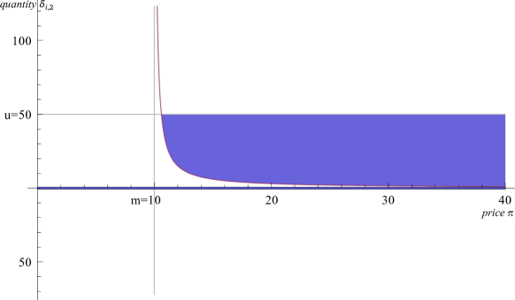
Figure 0.1: thick line and marked area: price-quantity combinations with a non-negative surplus.

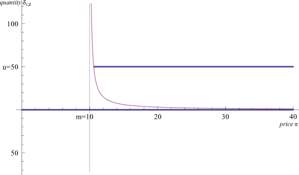
Figure 0.2: thick lines: quantities are either zero or maximize (SellBid)($\pi$).

Now assume that there is a convex demand bid $j$. The marginal willingness to pay amounts to ${20\,€}$/unit and the maximal demanded quantity amounts to $40$ units. The individual optimization problem is as follows:

$$\left(\begin{matrix}\hfill\max\quad&v_{j}(\delta_{j})-\pi^{\top}f_{j}(\delta_{j})\hfill\\ \hfill\mathop{\rm s.t.}\quad&\delta_{j}\in D_{j}\hfill\end{matrix}\right)=\left(\begin{matrix}\hfill\max\quad&20\delta_{j}-\pi^{\top}\delta_{j}\hfill\\ \hfill\mathop{\rm s.t.}\quad&\delta_{j}\in[0,40]\hfill\end{matrix}\right), \pi$$ (BuyBid)()

In Model A the sell bid either produces nothing or 50 units (cf. Figure 0.2). Therefore, the buy bid cannot be executed, because buys at most 40 units. Model A ends up with an economic surplus of zero Euro. If we replace the equation (0.76) by the less restrictive constraint (0.75), the following solution becomes feasible: $\delta_{i}=(1,40)$, $\delta_{j}=40$, and $\pi=15$. The solution generates an economic surplus of $20\cdot 40-30-10\cdot 40=370$ Euro. The sell bid $i$ has a non-negative surplus of $15\cdot 40-30-10\cdot 40=170$ Euro and the decision variable $\delta_{i}$ is feasible for (SellBid)($\pi$). The buy bid $j$ has a surplus of $20\cdot 40-15\cdot 40=200$ Euro and the decision variable $\delta_{j}$ maximizes (BuyBid)($\pi$).

The example shows that it may be disadvantageous to enforce constraint (0.76). This is done in Model A, which computes the trivial zero solution in the previous example. No bid is executed, even though there exists a solution where both participants have a strictly positive surplus. This is not desirable. To address this issue, one can consider the following relaxation of (MainMPEC).

$$\max\quad \sum_{i\in I}v_{i}(\delta_{i}),$$ (0.77)

$$\mathop{\rm s.t.}\quad \sum_{i\in I}f_{i,t}(\delta_{i})=0 \forall{t\in T},$$ (0.78)

$$\delta_{i}\in\arg\max\{v_{i}(\delta_{i}^{\prime})-{\pi}^{\top}f_{i}(\delta_{i}^{\prime})\mid\delta_{i}^{\prime}\in D_{i}\} \forall i\in I_{C},$$ (0.79)

$$\delta_{i}\in D_{i}\quad\text{ and }\quad v_{i}(\delta_{i})-{\pi}^{\top}f_{i}(\delta_{i})\geq 0 \forall i\in I_{N}.$$ (0.80)

This model ensures that the decision variables of each convex bid maximize the individual surplus and the decision variables of each non-convex bid are feasible and the associated surplus is non-negative. Similar to constraint (0.76) in model (MainMPEC), constraint (0.79) may lead to unfavorable solutions. Model (0.77)-(0.80) may compute the trivial zero solution, even if there exists a solution where all participants have a strictly positive surplus. These considerations lead to a further relaxation of (MainMPEC).

$$\max\quad \sum_{i\in I}v_{i}(\delta_{i}),$$ (NoLoss)

$$\mathop{\rm s.t.}\quad \sum_{i\in I}f_{i,t}(\delta_{i})=0 \forall{t\in T},$$

$$\delta_{i}\in D_{i}\quad\text{ and }\quad v_{i}(\delta_{i})-{\pi}^{\top}f_{i}(\delta_{i})\geq 0 \forall i\in I.$$

The model does not distinguish between convex and non-convex bids. It maximizes the economic surplus subject to the clearing condition, the feasibility of the decision variables, and the guarantee that no participant incurs a loss. Recall that $\delta$ and $\pi$ are the variables of the model. Therefore, the non-negative surplus constraint is non-convex, thus it is difficult to handle.

In the following paragraph we show that the diseconomies described above do not arise in the model (NoLoss). Therefore, we introduce an efficiency term that characterizes economically desirable solutions and takes the strict linear prices into account.

Definition 0.31.

A tuple $(\delta^{*},\pi^{*})$ is an efficient solution to the multicriteria optimization problem

$$\max\quad \begin{pmatrix}v_{1}(\delta_{1})-\pi^{\top}f_{1}(\delta_{1})\\ \vdots\\ v_{|I|}(\delta_{|I|})-\pi^{\top}f_{|I|}(\delta_{|I|})\end{pmatrix}$$ (Multi)

$$\mathop{\rm s.t.}\quad \sum_{i\in I}f_{i,t}(\delta_{i})=0 \forall{t\in T},$$

$$\delta_{i}\in D_{i} \forall i\in I,$$

$$\pi_{t}\in\mathbb R \forall{t\in T}$$

if there is no other feasible solution $(\delta,\pi)$ to (Multi) with

$$v_{i}(\delta_{i})-\pi^{\top}f_{i}(\delta_{i}) \geq v_{i}(\delta^{*}_{i})-{\pi^{*}}^{\top}f_{i}(\delta^{*}_{i}) \text{for all }i\in I\text{ and }$$ (0.81)

$$v_{i}(\delta_{i})-\pi^{\top}f_{i}(\delta_{i}) >v_{i}(\delta^{*}_{i})-{\pi^{*}}^{\top}f_{i}(\delta^{*}_{i}) \text{for some }i\in I.$$ (0.82)

In other words, $(\delta^{*},\pi^{*})$ is an efficient solution to (Multi) if the surplus of a participant cannot be increased without decreasing the surplus of another participant.

Proposition 0.32.

An optimal solution to (NoLoss) is an efficient solution to (Multi).

Proof.

Let $(\delta^{*},\pi^{*})$ be an optimal solution to (NoLoss). At this solution the surplus of each participant $i\in I$ is non-negative: $v_{i}(\delta^{*}_{i})-{\pi^{*}}^{\top}f_{i}(\delta^{*}_{i})\geq 0$. Assume that there is a feasible solution $(\delta,\pi)$ to (Multi) with (0.81) and (0.82). Equation (0.81) yields

$$v_{i}(\delta_{i})-\pi^{\top}f_{i}(\delta_{i})\geq v_{i}(\delta^{*}_{i})-{\pi^{*}}^{\top}f_{i}(\delta^{*}_{i})\geq 0\qquad\text{for all }i\in I.$$

In other words, $(\delta,\pi)$ is also a feasible solution to (NoLoss). We will now compare the objective values of both solutions.

$$\sum_{i\in I}v_{i}(\delta_{i})=\sum_{i\in I}\left(v_{i}(\delta_{i})-\pi^{\top}f_{i}(\delta_{i})\right)\mathop{>}\limits_{\overbrace{{\scriptstyle\eqref{eq efficient 1}\text{ and }\eqref{eq efficient 2}}}}\sum_{i\in I}\left(v_{i}(\delta^{*}_{i})-{\pi^{*}}^{\top}f_{i}(\delta^{*}_{i})\right)=\sum_{i\in I}v_{i}(\delta^{*}_{i}).$$

This is a contradiction, because $(\delta^{*},\pi^{*})$ maximizes (NoLoss). The objective value of $(\delta,\pi)$ cannot be strictly greater than the objective value of $(\delta^{*},\pi^{*})$.

An optimal solution to (NoLoss) is an allocation that maximizes the economic surplus such that there exists a strict linear pricing schedule where no participant incurs a loss. It is not possible to increase the surplus of one participant without decreasing the surplus of another participant. In particular any allocation with a higher economic surplus requires the use of another pricing schedule, because otherwise at least one participant incurs a loss. Due to these properties we call an optimal solution to (NoLoss) a strict linear price equilibrium.

4.3 Read-World Application

The previous models and algorithms are motivated by a real-world application. In our previous paper (Martin et al. (2013)) we modeled the European day-ahead electricity auction and developed an exact algorithm and a heuristic for this specific auction. The electricity auction model is similar to model (0.77)-(0.80). Even though the algorithms in Martin et al. (2013) are designed to solve the specific electricity auction problem, they can be generalized. The generalized algorithms can solve Model A for arbitrary mixed integer auctions (cf. Algorithm 4.1 in Section 4.1). Note that in general Model A differs from (0.77)-(0.80), and therefore, does not reflect all requirements of the electricity auction. However, the specialized algorithms in Martin et al. (2013) are similar to the ones in this paper. They are applicable to large scale real-world electricity auctions and produce high quality solutions in a short time.

5 Summary and Outlook

The article presents two relaxations of a competitive equilibrium in general auctions. For the first relaxation (MainMPEC)  we constructed an exact algorithm and a heuristic. Both algorithms are applicable to mixed integer auctions. Even though the first relaxation has desirable algorithmic properties, we showed that an optimal solution might not be efficient from an economical point of view: there exist situations, where all participants can be made better off. Such an improvement can be achieved if we replace all optimality conditions by the condition that no participant may incur a loss. This leads us to the second relaxation (NoLoss), which maximizes the economic surplus such that no participant incurs a loss. A solution to this model turns out to be efficient: no participant can be made better off without making another one worse off. The second relaxation is economically preferable, but the algorithms for the first relaxation, only provide heuristic solutions to the second relaxation. Further research could be concerned about algorithms that can solve large scale mixed integer auction instances of the second relaxation.

Appendix Appendix A. Convex Optimization

In this section we shortly introduce some basic definitions and results concerning convex optimization. Consider the convex optimization problem

$$\max\quad v(x),$$ (A.1)

$$\mathop{\rm s.t.}\quad f_{i}(x)=0 i=1,\dots,k,$$ (A.2)

$$g_{i}(x)\leq 0 i=1,\dots,m,$$ (A.3)

where $v,f_{i},g_{i}:\mathbb R^{n}\rightarrow\mathbb R$ are differentiable functions, $v$ concave, $g_{i}$ convex, and $f_{i}$ affine. To describe optimal solutions to this problem it is convenient to assume that the weak Slater assumption holds. Hiriart-Urruty & Lemaréchal (1993) provide the following definition:

Definition 0.33.

The constraints (A.2)-(A.3) satisfy the weak Slater assumption if there is a feasible point at which all the non-affine constraints are strictly satisfied, i.e., there exists $\hat{x}\in\mathbb R^{n}$ with

$$f_{i}(\hat{x}) =0 i=1,\dots,k,$$

$$g_{i}(\hat{x}) \leq 0 i=1,\dots,m\text{ and $g_{i}$ is affine},$$

$$g_{i}(\hat{x}) <0 i=1,\dots,m\text{ and $g_{i}$ is non-affine}.$$

With this assumption the Karush-Kuhn-Tucker conditions, short KKT conditions, are necessary and sufficient to describe an optimal solution to our convex problem:

Theorem 0.34 (KKT for differentiable convex problems).

Let $v,f_{i},g_{i}:\mathbb R^{n}\rightarrow\mathbb R$ be differentiable functions, $v$ concave, $g_{i}$ convex, and $f_{i}$ affine. If for $\bar{x},\bar{}\pi,\bar{\lambda}$ the KKT conditions

$$f_{i}(\bar{x}) =0 i=1,\dots,k,$$ (A.4)

$$g_{i}(\bar{x}) \leq 0 i=1,\dots,m,$$ (A.5)

$$\sum_{i=1}^{k}\bar{}\pi_{i}\frac{\partial f_{i}}{\partial x_{j}}(\bar{x})+\sum_{i=1}^{m}\bar{\lambda}_{i}\frac{\partial g_{i}}{\partial x_{j}}(\bar{x}) =\frac{\partial v}{\partial x_{j}}(\bar{x}) j=1,\dots,n,$$ (A.6)

$$\bar{\lambda}_{i} \geq 0 i=1,\dots,m,$$ (A.7)

$$\bar{\lambda}_{i}g_{i}(\bar{x}) =0 i=1,\dots,m,$$ (A.8)

hold, then $\bar{x}$ is primal optimal and $(\bar{}\pi,\bar{\lambda})$ dual optimal for (A.1)-(A.3). If $\bar{x}$ is primal optimal and the weak Slater assumption holds, then there exists $(\bar{}\pi,\bar{\lambda})$ such that the KKT conditions are satisfied.

Proof.

Confer Theorem VII.2.1.4 and VII.2.2.5 in Hiriart-Urruty & Lemaréchal (1993) or Chapter 5.5.3 in Boyd & Vandenberghe (2004).

Proposition 0.35.

Let $v,f_{i},g_{i}:\mathbb R^{n}\rightarrow\mathbb R$ be differentiable functions, $v$ concave, $g_{i}$ convex, and $f_{i}$ affine. Let $\bar{x}$ and $\bar{x}^{\prime}$ be optimal solutions to (A.1)-(A.3) and let $M(\bar{x}):=\{(\bar{}\pi,\bar{\lambda})\mid\eqref{eq cp dual 1}-\eqref{eq cp dual 3}\}$. Then $M(\bar{x})=M(\bar{x}^{\prime})$.

Proof.

Confer Proposition VII.3.3.1 in Hiriart-Urruty & Lemaréchal (1993).

References

- Balas (1979) Balas, E. (1979). Disjunctive programming. Annals of Discrete Mathematics, 5, 3–51. Discrete optimization II (Proc. Adv. Res. Inst. Discrete Optimization and Systems Appl., Banff, Alta., 1977).
- Blumrosen & Nisan (2007) Blumrosen, L., & Nisan, N. (2007). Combinatorial Auctions. In N. Nisan, T. Roughgarden, É. Tardos, & V. V. Vazirani (Eds.), Algorithmic Game Theory chapter 11. (pp. 267–299). New York: Cambridge University Press.
- Boyd & Vandenberghe (2004) Boyd, S., & Vandenberghe, L. (2004). Convex Optimization. Cambridge: Cambridge University Press.
- De Vries & Vohra (2003) De Vries, S., & Vohra, R. V. (2003). Combinatorial Auctions: A Survey. INFORMS Journal on Computing, 15, 284–309. doi:10.1287/ijoc.15.3.284.16077.
- Geoffrion (1972) Geoffrion, A. M. (1972). Generalized Benders decomposition. Journal of Optimization Theory and Applications, 10, 237–260. doi:10.1007/BF00934810.
- Hiriart-Urruty & Lemaréchal (1993) Hiriart-Urruty, J.-B., & Lemaréchal, C. (1993). Convex analysis and minimization algorithms. I. Fundamentals volume 305 of Grundlehren der Mathematischen Wissenschaften [Fundamental Principles of Mathematical Sciences]. Berlin: Springer-Verlag.
- Martin et al. (2013) Martin, A., Müller, J., & Pokutta, S. (2013). Strict Linear Prices in Non-Convex European Day-Ahead Electricity Markets. Optimization Methods and Software, . doi:10.1080/10556788.2013.823544.
- Mas-Colell et al. (1995) Mas-Colell, A., Whinston, M. D., & Green, J. R. (1995). Microeconomic Theory. New York: Oxford University Press.
- O’Neill et al. (2005) O’Neill, R., Sotkiewicz, P., Hobbs, B., Rothkopf, M., & Stewart, W. (2005). Efficient market-clearing prices in markets with nonconvexities. European Journal of Operational Research, 164, 269–285.
- Tirole (1988) Tirole, J. (1988). The Theory of Industrial Organization. Cambridge: MIT Press.
- Van Vyve (2011) Van Vyve, M. (2011). Linear prices for non-convex electricity markets: models and algorithms. CORE Discussion Papers 2011050 Université catholique de Louvain, Center for Operations Research and Econometrics (CORE). URL: http://EconPapers.repec.org/RePEc:cor:louvco:2011050.