Hawking radiation in a two-component Bose-Einstein condensate

Abstract

We consider a simple realization of an event horizon in the flow of a one-dimensional two-component Bose-Einstein condensate. Such a condensate has two types of quasiparticles; In the system we study, one corresponds to density fluctuations and the other to polarization fluctuations. We treat the case in which a horizon occurs only for one type of quasiparticles (the polarization ones). We study the one- and two-body signal associated to the analog of spontaneous Hawking radiation and demonstrate by explicit computation that it consists only in the emission of polarization waves. We discuss the experimental consequences of the present results in the domain of atomic Bose-Einstein condensates and also for the physics of exciton-polaritons in semiconductor microcavities.

An intense research activity has been developed in the recent years aiming at identifying Hawking radiation in several analog models of gravity (see refs. [1, 2] for recent reviews). The possible black hole configurations realized in an analogous system all rely on the remark by Unruh [3] that if the flow of a fluid has, while remaining stationary, a transition from a subsonic upstream region to a supersonic downstream region, the interface between these two regions behaves as an event horizon for sound waves. The supersonic region mimics the interior of a black hole since no sound can escape from it (one speaks of “dumb hole”). This analogy is richer than a mere realization of a sonic event horizon: Quantum virtual particles can tunnel out near the horizon and are then separated by the background flow giving rise to correlated currents emitted away from the region of the horizon (both inside and outside of the black hole), in exact correspondence with the original scenario of Hawking radiation [4].

Among the prominent experimental configurations where a sonic horizon has been realized one can quote the use of ultrashort pulses moving in optical fibers [5] or in a dielectric medium [6], the study of the flow of a Bose-Einstein condensate (BEC) past an obstacle [7], of a laser propagating in a nonlinear luminous liquid [8], or of surface waves on moving water [9, 10]. Several recent theoretical works proposed other realizations of an artificial event horizon, using for instance an electromagnetic wave guide [11] (or more recently a SQUID array transmission line [12]), ring-shaped chain of trapped ions [13], graphene [14, 15], or edge modes of the filling fraction $\nu=1$ quantum Hall system [16]. Among these theoretical proposals, those employing an exciton-polariton superfluid [17, 18] deserve special attention because they could be realized in a near future. Such systems are specific because polaritons have an effective spin $1/2$ and, as we will see below, this has important qualitative consequences on the expected Hawking signal.

In the present work we study the possible signatures of Hawking radiation in a generic two-component BEC system. Such a system is peculiar in the sense that it sustains two types of elementary excitations, with different long-wavelength velocities. This makes it possible to realize a unique configuration where an event horizon occurs for one type of excitations but not for the other. The associated artificial black hole could be experimentally implemented in a polariton condensate (such as proposed in ref. [18]), but also in a two-species BEC such as realized by considering for instance ⁸⁷Rb in two hyperfine states [19], or a mixture of two elements [20], or different isotopes of the same atom [21]. A general theory of such systems requires to consider a wide range of parameters and of different situations corresponding to possibly different masses of the two species, to different strengths and signs of intra- and inter-species interactions, to different types of external potentials (possibly species-dependent) and of coupling between the two components. In the present work we consider a simple model which captures the essential physical ingredients and characteristics of the phenomenon: The order parameter of the two-component BEC is described by a one-dimensional (1D) two-component Heisenberg field operator $(\hat{\psi}_{+}(x,t),\hat{\psi}_{-}(x,t))$ obeying a set of coupled Gross-Pitaevskii equations:

$${\rm i}\hbar\,\partial_{t}\hat{\psi}_{\pm}= -\frac{\hbar^{2}}{2m}\,\partial_{x}^{2}\hat{\psi}_{\pm}+U(x)\,\hat{\psi}_{\pm}$$

$$+\big{[}g_{1}\,\hat{n}_{\pm}+g_{2}(x)\,\hat{n}_{\mp}\big{]}\,\hat{\psi}_{\pm}-\mu\,\hat{\psi}_{\pm}\,.$$ (1)

In this equation $\hat{n}_{\pm}(x,t)=\hat{\psi}^{\dagger}_{\pm}(x,t)\,\hat{\psi}_{\pm}(x,t)$ is the density of the $(\pm)$-component, $U(x)$ is an external potential, $\mu$ is the chemical potential, and $g_{1}$ ($g_{2}$) is the intra-species (inter-species) contact-interaction coupling constant. We choose to work in a configuration where $0<g_{2}<g_{1}$. This is quite realistic for atomic condensates (provided one neglects the small difference of the interaction constant between $+/+$ and $-/-$ components). For excitonic polaritons it is accepted that $g_{1}>0$ and that $|g_{2}|<g_{1}$, in agreement with the observed overall repulsion between polaritons, but it is typically believed that $g_{2}<0$. However, depending on the detuning between the photon and the exciton modes (and on the proximity with the bi-exciton resonance), $g_{2}$ may be positive or negative, as observed in refs. [22, 23]. Our choice to consider the case of a positive $g_{2}$ parameter will make it possible to treat a setting where the event horizon occurs for a flow velocity inferior to the one of ordinary sound.

We consider an idealized model in which $g_{2}$ and the external potential $U$ both depend on $x$ in a way that ensures the existence of a homogeneous and stationary classical solution of eq. (Hawking radiation in a two-component Bose-Einstein condensate) of the form

$$\Psi_{\pm}(x)=\sqrt{n_{0}/2}\,\exp({\rm i}k_{0}x)\,.$$ (2)

This can be realized by considering a step-like configuration for which $U(x)=U_{u}\,\Theta(-x)+U_{d}\,\Theta(x)$ and $g_{2}(x)=g_{2,u}\,\Theta(-x)+g_{2,d}\,\Theta(x)$ (where $\Theta$ is the Heaviside step function) with

$$U_{u}+g_{2,u}\,n_{0}/2=U_{d}+g_{2,d}\,n_{0}/2.$$ (3)

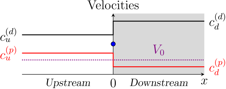
Figure 1: (Colour on-line) Velocities of the ordinary sound $c^{(d)}$ (black solid line) and of the polarization sound $c^{(p)}$ (red solid line) as a function of $x$. The dotted horizontal line represents the constant velocity $V_{0}$ of the flow. The blue dot is the reference velocity $\sqrt{g_{1}n_{0}/(2m)}$. The downstream region is shaded in order to recall that it corresponds to the interior of the black hole.

The order parameter (2) describes a uniform flow in which both components have the same density $n_{0}/2$ and the same velocity $V_{0}=\hbar k_{0}/m$. We consider the case $V_{0}>0$, and denote the $x<0$ ($x>0$) region as the upstream (downstream) region. In each of these regions the long-wavelength elementary excitations consist either in density or in polarization fluctuations with respective velocities denoted as $c_{\alpha}^{(d)}$ and $c_{\alpha}^{(p)}$ ($\alpha=u$ or $d$, depending if one considers the upstream or the downstream region). $c_{\alpha}^{(d)}$ is the usual speed of sound whereas $c_{\alpha}^{(p)}$ will be termed “polarization sound velocity”; Their precise definition will be given later [after Eqs. (6) and (7)]. As illustrated in fig. 1 we choose the parameters of the system in such a way that

$$c_{d}^{(p)}<V_{0}<c_{u}^{(p)}<c_{u}^{(d)}<c_{d}^{(d)}\,.$$ (4)

Then the point $x=0$ is an event horizon for the fluctuations of polarization but not for the fluctuations of density (the usual sound).

Note that the configuration we consider is of the same type as the one considered in refs. [24, 25] for a one-component system, and seems rather awkward: It consists in a uniform flow of a 1D BEC in which the two-body interaction varies spatially (in order to locally modify the speed of polarization sound in the system) although the velocity and the density of the flow remain constant. This is only possible in the presence of an external potential specially tailored so that the local chemical potential remains constant everywhere [this is ensured by eq. (3)]. This makes the whole system quite difficult to realize experimentally. However, it was shown in refs. [26] and [18] that the Hawking radiation associated to this configuration has the same properties as others associated to more realistic realizations of an event horizon in a BEC or a polariton condensate.

Figure 2: (Colour on-line) Upstream (upper plot) and downstream (middle plot) dispersion relations. The red (black) curves correspond to polarization (density) modes. In each plot the horizontal dashed line is fixed by the chosen value of $\omega$. The labeling of the different branches is explained in the text. The abscissae of the dots fix the values of the wavevector $q(\omega)$ corresponding to each branch. The lower diagram illustrates the terminology used in the main text for denoting the waves as outgoing or ingoing. As in fig. 1, the downstream region is shaded in order to recall that it corresponds to the interior of the black hole.

The black hole configuration being fixed, we now characterize the spontaneous Hawking emission by studying the quantum Bogoliubov excitations of the system, in a manner similar to what has been done in refs. [27, 28, 29]. The most efficient way to characterize the different branches of the dispersion relation is to consider the classical (or more precisely first quantized) version of eq. (Hawking radiation in a two-component Bose-Einstein condensate). One writes the order parameter as $\psi_{\pm}(x,t)=\Psi_{\pm}(x)+\delta\psi_{\pm}(x,t)$ with $|\delta\psi_{\pm}|\ll|\Psi_{\pm}|$. In a region where $U(x)$ and $g_{2}(x)$ have the constant value $U_{\alpha}$ and $g_{2,\alpha}$ ($\alpha=u$ or $d$) the fluctuations with given pulsation $\omega$ on top of the background (2) are of the form

$$\delta\psi_{\pm}(x,t)=\mathrm{e}^{{\rm i}k_{0}x}\big{[}u_{\pm,\alpha}(x,\omega)\,\mathrm{e}^{-{\rm i}\omega t}+w_{\pm,\alpha}^{*}(x,\omega)\,\mathrm{e}^{{\rm i}\omega t}\big{]}\,,$$ (5)

where the $u_{\pm,\alpha}$’s and the $w_{\pm,\alpha}$’s are plane waves of momentum $\hbar\,q$. The corresponding dispersion relations are represented in fig. 2. The curves corresponding to density fluctuations are represented in black in the figure. Their dispersion relation reads

$$(\omega-V_{0}\,q)^{2}=[c_{\alpha}^{(d)}]^{2}q^{2}+\frac{\hbar^{2}q^{4}}{4m^{2}}\,,$$ (6)

with $m[c_{\alpha}^{(d)}]^{2}=\frac{1}{2}(g_{1}+g_{2,\alpha})n_{0}$ ($\alpha=u$ or $d$). In the left-hand side of eq. (6) the term $-V_{0}\,q$ is a Doppler shift indicating that the dispersion relation is evaluated in the laboratory frame in which the flow has a constant and uniform velocity $V_{0}$. In the upstream region the different channels corresponding to (6) are denoted as $u^{(d)}|{\rm in}$ and $u^{(d)}|{\rm out}$, where the $u$ stands for “upstream”, the $(d)$ for “density” and the “in” (the “out”) labels the wave whose group velocity is directed towards (away from) the horizon. What is considered as an ingoing or an outgoing wave is pictorially represented in the lower diagram of fig. 2. In the downstream region the channels are accordingly denoted as $d^{(d)}|{\rm in}$ and $d^{(d)}|{\rm out}$ (see fig. 2).

The curves corresponding to fluctuations of the polarization [$\pi(x,t)=n_{+}(x,t)-n_{-}(x,t)$] are represented in red in figure 2. Their dispersion relation is

$$(\omega-V_{0}\,q)^{2}=[c_{\alpha}^{(p)}]^{2}q^{2}+\frac{\hbar^{2}q^{4}}{4m^{2}}\,,$$ (7)

with $m[c_{\alpha}^{(p)}]^{2}=\frac{1}{2}(g_{1}-g_{2,\alpha})n_{0}$. In the upstream region the corresponding channels are denoted as $u^{(p)}|{\rm in}$ and $u^{(p)}|{\rm out}$. In the downstream region, $V_{0}>c_{d}^{(p)}$, and new branches appear in the dispersion relation of polarization waves. Altogether in this region the branches are denoted as $d1^{(p)}|{\rm in}$, $d1^{(p)}|{\rm out}$, $d2^{(p)}|{\rm in}$ and $d2^{(p)}|{\rm out}$ (see fig. 2). In the following we refer to the quasiparticles corresponding to the dispersion relation (6) as density quasiparticles and to those corresponding to (7) as polarization quasiparticles.

The existence of the discontinuity in the parameters of the system at $x=0$ prevents the channels we have just identified for an hypothetical homogeneous configuration to be the true eigenmodes of the system. The correct eigenmodes are linear combinations of the channels in the upstream region and channels in the downstream one, with appropriate matching at $x=0$. Among all the possible combinations, we are primarily interested in the scattering modes which describe a plane-wave excitation originating from infinity – either upstream or downstream – on a well defined ingoing channel, impinging on the horizon, and then leaving again towards infinity as a superposition of the outgoing branches. When $\omega$ is lower than the threshold $\omega_{*}$ identified in fig. 2, there are 5 ingoing channels and 5 outgoing ones. The corresponding scattering amplitudes form a $5\times 5$ $S$ matrix which can be shown to be block diagonal:

$$S=\left(\begin{array}[]{c|c}S^{(p,p)}&\begin{array}[]{cc}0&0\\ 0&0\\ 0&0\end{array}\\ \hline\cr\begin{array}[]{ccc}0&0&0\\ 0&0&0\end{array}&S^{(d,d)}\end{array}\right),$$ (8)

with

$$S^{(p,p)}=\left(\begin{array}[]{ccc}S_{u^{(p)},u^{(p)}}&S_{u^{(p)},d1^{(p)}}&S_{u^{(p)},d2^{(p)}}\\ S_{d1^{(p)},u^{(p)}}&S_{d1^{(p)},d1^{(p)}}&S_{d1^{(p)},d2^{(p)}}\\ S_{d2^{(p)},u^{(p)}}&S_{d2^{(p)},d1^{(p)}}&S_{d2^{(p)},d2^{(p)}}\end{array}\right),$$ (9d)

$$S^{(d,d)}=\left(\begin{array}[]{cc}S_{u^{(d)},u^{(d)}}&S_{u^{(d)},d^{(d)}}\\ S_{d^{(d)},u^{(d)}}&S_{d^{(d)},d^{(d)}}\\ \end{array}\right).$$ (9g)

For instance the $S_{u^{(p)},d1^{(p)}}$ matrix element denotes the (complex and $\omega$-dependent) scattering coefficient from the ingoing downstream channel $d1^{(p)}|{\rm in}$ towards the outgoing upstream channel $u^{(p)}|{\rm out}$. As discussed in refs. [29, 28, 26], current conservation imposes a skew unitarity of the $S$ matrix: $S^{\dagger}\eta S=\eta$, where here $\eta={\rm diag}(1,1,-1,1,1)$. When $\omega$ is larger than the maximum $\omega_{*}$ of the $d2^{(p)}$ branches (see fig. 2) the $d2|{\rm in}$ and $d2|{\rm out}$ channels disappear, the $S^{(p,p)}$ submatrix becomes $2\times 2$, and the now $4\times 4$ $S$ matrix obeys the usual unitarity condition $S^{\dagger}S={\rm diag}(1,1,1,1)$.

We computed the coefficients of the $S$ matrix both analytically (in the low-$\omega$ limit) and numerically (for unrestricted values of $\omega$). We checked the excellent agreement between the two approaches in their common range of validity (i.e., at $\omega\to 0$) and also that the current conservation conditions are verified, exactly in the analytical approach, and with a high degree of accuracy in the numerical treatment (the error is always less than $10^{-7}$). All the matrix coefficients of the form $S_{i,d1^{(p)}}$ and $S_{i,d2^{(p)}}$ with $i\in\{u^{(p)},d1^{(p)},d2^{(p)}\}$ (i.e., the two right most columns of $S^{(p,p)}$) diverge at low $\omega$. This is connected to the fact that the associated Wigner time delay diverges: Low-energy polarization quasiparticles entering the system via the $d1^{(p)}|{\rm in}$ or the $d2^{(p)}|{\rm in}$ channels – i.e., from the interior of the black hole – remain blocked at the horizon forever: This is a signature of the occurrence of an event horizon for the polarization modes. On the contrary, low-energy density quasiparticles entering the system from the downstream region can escape the black hole, since we work in a configuration where the horizon does not affect the density fluctuations (see fig. 1). Of course all quasiparticles entering the system from the upstream region can cross the horizon and penetrate into the black hole.

Within the present Bogoliubov analysis, the knowledge of the $S$ matrix of the system makes it possible to characterize the Hawking signal which corresponds to emission of radiation from the interior toward the exterior of the black hole. In our specific case the energy current associated to emission of elementary excitations is (cf. [30])

$$Q(x,t)=-\frac{\hbar^{2}}{2m}\sum_{\sigma=\pm 1}\left\langle\partial_{t}\hat{\psi}_{\sigma}^{\dagger}(x,t)\,\partial_{x}\hat{\psi}_{\sigma}(x,t)\right\rangle+{\rm H.c.}\,,$$ (10)

where “H.c.” stands for “Hermitian conjugate”. $Q(x,t)$ is here time and position-independent in agreement with the conservation of the energy flux in a stationary configuration. Computing its expression far upstream ($x\to-\infty$) one can show, as expected, that the current is only carried by the $u^{(p)}|{\rm out}$ channel and is, at zero temperature, given by the formula

$$Q=-\int_{0}^{\omega_{*}}\frac{{\rm d}\omega}{2\pi}\,\hbar\omega\,\big{|}S_{u^{(p)},d2^{(p)}}(\omega)\big{|}^{2}\,.$$ (11)

Hence the quantity $|S_{u^{(p)},d2^{(p)}}(\omega)|^{2}$ characterizes the emission spectrum of Hawking radiation. Although we consider a setting with step-like variations of the external parameters, resulting in an infinite effective surface gravity, the Hawking spectrum is still thermal like, i.e., approximately of the form

$$\big{|}S_{u^{(p)},d2^{(p)}}(\omega)\big{|}^{2}\simeq\frac{\Gamma}{\exp\big{(}\frac{\hbar\,\omega}{k_{\rm B}T_{\rm H}}\big{)}-1}\,,$$ (12)

where $k_{\rm B}$ is the Boltzmann constant, $\Gamma$ is denoted as the gray-body factor and $T_{\rm H}$ is the Hawking temperature. Since we have computed the explicit low-$\omega$ expression of the coefficients of the $S$ matrix, we can determine $T_{\rm H}$ and $\Gamma$ by a low-$\omega$ fit of expression (12). In particular one obtains the following explicit expressions for the reduced Hawking temperature ${\mathcal{T}}_{\rm H}=k_{\rm B}T_{\rm H}/m[c^{(p)}_{u}]^{2}$ and for the gray-body factor:

$${\mathcal{T}}_{\rm H}=\displaystyle{\frac{1}{2}\frac{\mathpzc{m}_{u}^{2}}{\mathpzc{m}_{d}}\frac{(1-\mathpzc{m}_{u}^{2})(\mathpzc{m}_{d}^{2}-1)^{\frac{3}{2}}}{\mathpzc{m}_{d}^{2}-\mathpzc{m}_{u}^{2}}}\,,\quad\Gamma=\frac{4\mathpzc{m}_{u}}{(1+\mathpzc{m}_{u})^{2}}\,,$$ (13)

where $\mathpzc{m}_{\alpha}=V_{0}/c^{(p)}_{\alpha}$ is the (polarization) Mach number in region $\alpha$ ($\alpha=u$ or $d$ and $\mathpzc{m}_{u}<1<\mathpzc{m}_{d}$).

The numerically determined $|S_{u^{(p)},d2^{(p)}}|^{2}$ is compared in fig. (3) with the thermal spectrum (12) where $T_{\rm H}$ is given by (13). The plot is done in a configuration where $\mathpzc{m}_{u}=0.7$, $\mathpzc{m}_{d}=3$ and $g_{2,u}/g_{1}=0.2$. In the type of setting we consider, fixing these three parameters determines all the other relevant quantities of the system. In particular one has here $g_{2,d}/g_{1}\simeq 0.956$, $V_{0}/c^{(d)}_{u}\simeq 0.572$ and $V_{0}/c^{(d)}_{d}\simeq 0.448$. As expected one sees in the figure that the (numerically) exact spectral density $|S_{u^{(p)},d2^{(p)}}|^{2}$ coincides with a thermal gray-body emission at low energy. Note however that $|S_{u^{(p)},d2^{(p)}}|^{2}$ is strictly zero for $\omega>\omega_{*}$ since above this threshold the $d2^{(p)}|{\rm in}$ and $d2^{(p)}|{\rm out}$ channels disappear and the $S$ matrix becomes $4\times 4$.

Figure 3: (Colour on-line) $|S_{u^{(p)},d2^{(p)}}|^{2}$ (red solid line) and its approximation by eq. (12) (black dashed line) as a function of $\omega$. We consider the case with $\mathpzc{m}_{u}=0.7$ and $\mathpzc{m}_{d}=3$. With the present choice of parameters, $\Gamma\simeq 0.969$, ${\mathcal{T}}_{\rm H}\simeq 0.111$ and $\omega_{*}\xi_{u}^{(p)}/c_{u}^{(p)}\simeq 0.196$, where $\xi_{u}^{(p)}=\hbar/(mc_{u}^{(p)})$. The inset displays ${\mathcal{T}}_{\rm H}$ as a function of $\mathpzc{m}_{u}$ for several values of $\mathpzc{m}_{d}$ ($\mathpzc{m}_{d}=1.5,\ldots,10$).

Formulas (13) show that the Hawking temperature is roughly of order of $m[c^{(p)}_{u}]^{2}$, which itself is of order of the chemical potential of the system. In atomic condensates the chemical potential is of order of the temperature of the system and the Hawking current will be hidden by the thermal noise. In polariton systems the chemical potential is typically of order of $0.5$ meV and low temperature experiments could in principle distinguish the Hawking current from the thermal noise.

We now consider an other experimental observable which can reveal the Hawking phenomenon even in the presence of a realistic thermal noise. As first explicitly pointed out in refs. [24, 25], in analog systems an external observer is able to measure correlations across the horizon revealing the existence of the Hawking current (see also refs. [28, 29, 31, 32, 26]). For the present setting we expect that these correlations are due to pair-wise emission of polarization quasiparticles on both sides of the horizon. The polarization density operator in our system is $\hat{\pi}(x,t)=\hat{n}_{+}(x,t)-\hat{n}_{-}(x,t)$. In the configuration we consider it has zero mean [$\langle\hat{\pi}(x,t)\rangle=0$] and the corresponding correlation signal is time-independent:

$$\begin{split}g^{(p)}(x,x^{\prime})&=\langle:\!\hat{\pi}(x,t)\,\hat{\pi}(x^{\prime},t)\!:\rangle\\ &=\langle\hat{\pi}(x,t)\,\hat{\pi}(x^{\prime},t)\rangle-\delta(x-x^{\prime})\,n_{0}\,.\end{split}$$ (14)

It is also interesting to study the correlation of the density fluctuations

$$\begin{split}g^{(d)}(x,x^{\prime})&=\langle:\!\delta\hat{n}(x,t)\,\delta\hat{n}(x^{\prime},t)\!:\rangle\\ &=\langle\delta\hat{n}(x,t)\,\delta\hat{n}(x^{\prime},t)\rangle-\delta(x-x^{\prime})\,n_{0}\,,\end{split}$$ (15)

where $\delta\hat{n}(x,t)=\hat{n}_{+}(x,t)+\hat{n}_{-}(x,t)-n_{0}$.

In a hypothetical homogeneous configuration where $U(x)$ and $g_{2}(x)$ have constant uniform values, these correlator read

$$g^{(d,p)}(x,x^{\prime})=\frac{n_{0}}{\xi^{(d,p)}}\,F\left(\frac{|x-x^{\prime}|}{\xi^{(d,p)}}\right),$$ (16)

where $F(z)=-(\pi z)^{-1}\int_{0}^{\infty}{\rm d}t\,\sin(2\,t\,z)\,(1+t^{2})^{-3/2}$ and $\xi^{(d,p)}=\hbar/mc^{(d,p)}$.

The correlation patterns (16) are drastically modified in the presence of an event horizon. There is a first trivial modification due to the space dependence of the speeds of sound: Formulas (16) are modified upstream and downstream of the horizon because, in the region $x<0$, the values of $\xi^{(d)}_{u}$ and $\xi^{(p)}_{u}$ are different from those of $\xi^{(d)}_{d}$ and $\xi^{(p)}_{d}$ in the region $x>0$. The second modification corresponds to long-distance correlations and is more interesting: Quantum fluctuations generate correlated currents of polarization quasiparticles propagating away from the horizon in the $u^{(p)}|{\rm out}$, $d1^{(p)}|{\rm out}$ and $d2^{(p)}|{\rm out}$ channels. This, in turn, induces long-range modifications of $g^{(p)}(x,x^{\prime})$. No such long-distance correlations are expected for $g^{(d)}(x,x^{\prime})$ since there is no horizon for the density quasiparticles.

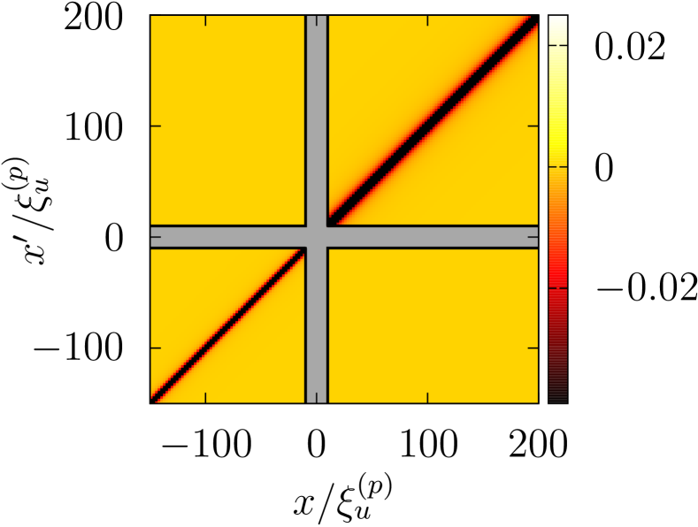
Figure 4: (Colour on-line) 2D plot of the numerical result for the dimensionless quantity $\xi_{u}^{(p)}g^{(d)}(x,x^{\prime})/n_{0}$ in the case in which $g_{2,u}/g_{1}=0.2$, $\mathpzc{m}_{u}=0.7$ and $\mathpzc{m}_{d}=3$. The shaded area near the axis corresponds to the zone $|x|$ or $|x^{\prime}|<10\,\xi_{u}^{(p)}$.

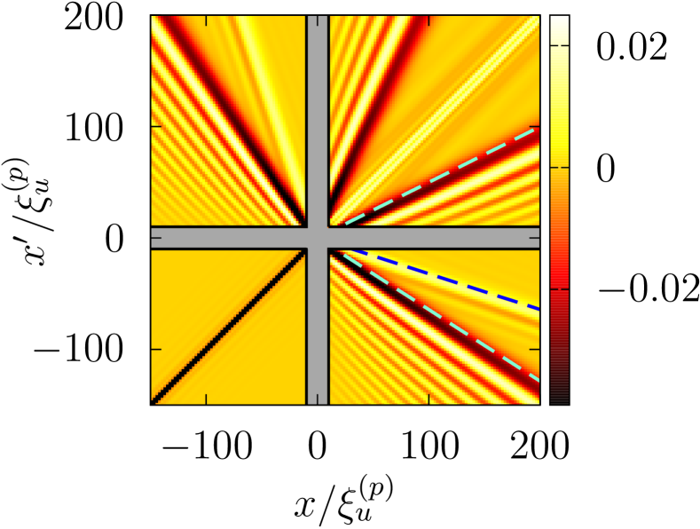
Figure 5: (Colour on-line) Same as fig. 4 for the dimensionless quantity $\xi_{u}^{(p)}g^{(p)}(x,x^{\prime})/n_{0}$. The dashed straight lines correspond to the correlation lines where a heuristic interpretation of the Hawking signal leads to expecting the largest long-range signal (see the text).

The knowledge of the $S$ matrix makes it possible to explicitly compute the quantities $g^{(p)}(x,x^{\prime})$ and $g^{(d)}(x,x^{\prime})$ if $x$ and $x^{\prime}$ are not too close to the horizon. We do not write down here the extensive explicit formulas (see ref. [33]) but rather display a plot of both quantities $g^{(d)}(x,x^{\prime})$ (fig. 4) and $g^{(p)}(x,x^{\prime})$ (fig. 5) in a black hole configuration with $g_{2,u}/g_{1}=0.2$, $\mathpzc{m}_{u}=0.7$ and $\mathpzc{m}_{d}=3$ (the same parameters for which fig. 3 has been drawn). As expected no track of Hawking radiation can be observed in the plot of $g^{(d)}(x,x^{\prime})$. On the other hand, $g^{(p)}(x,x^{\prime})$ displays long-range correlations along three special directions highlighted in fig. 5 by dashed straight lines. According to the standard scenario of Hawking radiation[4], if correlated low-energy Hawking quasiparticles are emitted along the $u^{(p)}|{\rm out}$, $d1^{(p)}|{\rm out}$ and $d2^{(p)}|{\rm out}$ channels, at time $t$ after their emission, these phonons are respectively located at positions $(V_{0}-c_{u}^{(p)})\,t<0$ , $(V_{0}+c_{d}^{(d)})\,t>0$, and $(V_{0}-c_{d}^{(p)})\,t>0$. This induces a correlation signal along the lines of slopes $(V_{0}-c_{u}^{(p)})/(V_{0}+c_{d}^{(p)})$ (resulting from correlations between phonons emitted along the $u^{(p)}$ and $d1^{(p)}$ outgoing channels), $(V_{0}-c_{u}^{(p)})/(V_{0}-c_{d}^{(p)})$ ($u^{(p)}|{\rm out}-d2^{(p)}|{\rm out}$ correlations), and $(V_{0}-c_{d}^{(p)})/(V_{0}+c_{d}^{(p)})$ ($d2^{(p)}|{\rm out}-d1^{(p)}|{\rm out}$ correlations). These are the three slopes marked by dashed lines in fig. 5. These large-distance correlation lines are accompanied by diffractive corrections building an oscillatory pattern in their vicinity (see, e.g., the discussion in ref.  [29]). Of course the lines with inverse slopes are also present (they correspond to the exchange $x\leftrightarrow x^{\prime}$ in fig. 5). The fact that, in the present setting, such a pattern is observed in the correlation of polarization fluctuations but not in the correlation of density fluctuations is a strong demonstration that this signal is intrinsically connected to Hawking radiation and requires the occurrence of a horizon.

The experimental detection of the polarization signal described in the present work is simple in the case of a polariton condensate because the pseudo-spin of the decaying polaritons is commuted into right or left circular polarization of the emitted photons. Also, the high repetition rate achieved in this type of experiment should make it possible to obtain a good statistics leading to a precise evaluation of the correlation signal. For atomic condensates on the other hand, the imaging techniques may rely on Stern-Gerlach and time-of-flight analysis or dispersive optical measurements [34] (for a review, see, e.g., [35]).

Finally we note that the present treatment of vacuum fluctuations in a stationary configuration, which is valid for a stable/conservative atomic condensate, does not immediately apply for a nonequilibrium polariton condensate. Indeed polaritons have a finite lifetime and the vacuum fluctuations such as described in the present stationary situation strictly speaking disappear, because no ingoing mode issued from infinity is able to reach the horizon. The fluctuations of the system are now triggered by fluctuations inside the excitonic reservoir and by the losses. A related view concerns the dispersion relation plotted in fig. 2: Because of damping, the frequency of the normal modes typically acquire an imaginary part, and long-wavelength density modes even become completely diffusive (see, e.g., the review [36]). However, one can show, within a simple model of nonresonant pumping with gain and loss, that these damping effects which are indeed present in the density channel, only weakly affect the polarization mode [37] and we thus expect that the results of the present work should be also observable in future experiments on out-of-equilibrium polariton condensates.

1 3

Carusotto I. Mueller E. J. J. Phys. B: At. Mol. Opt. Phys.372004S115

Stamper-Kurn D. M. Ueda M. Rev. Mod. Phys.8520131191

Carusotto I. Ciuti C. Rev. Mod. Phys.852013299

Larré P.-É., Pavloff N. Kamchatnov A. M. arXiv:1309.34942013

- [1] \NameBarceló C., Liberati S. Visser M. \REVIEWLiving Rev. Relativity1420113
- [2] \NameRobertson S. J. \REVIEWJ. Phys. B: At. Mol. Opt. Phys. 452012163001
- [3] \NameUnruh W. G. \REVIEWPhys. Rev. Lett.4619811351
- [4] \NameHawking S. W. \REVIEWCommun. Math. Phys.431975199
- [5] \NamePhilbin T. G., Kuklewicz C., Robertson S., Hill S., König F. Leonhardt U. \REVIEWScience31920081367
- [6] \NameBelgiorno T. et al. \REVIEWPhys. Rev. Lett.1052010203901
- [7] \NameLahav O. et al. \REVIEWPhys. Rev. Lett.1052010240401
- [8] \Name Elazar M., Fleurov V., Bar-Ad S. \REVIEWPhys. Rev. A862012063821
- [9] \NameRousseaux G., Mathis C., Maïssa P., Philbin T. G. Leonhardt U. \REVIEWNew J. Phys.102008053015
- [10] \NameWeinfurtner S., Tedford E. W., Penrice M. C. J., Unruh W. G. Lawrence G. A. \REVIEWPhys. Rev. Lett.1062011021302
- [11] \NameSchützhold R. Unruh W. G. \REVIEWPhys. Rev. Lett.952005031301
- [12] \NameNation P. D., Blencowe M. P., Rimberg A. J. Buks E. \REVIEWPhys. Rev. Lett.1032009087004
- [13] \NameHorstmann B., Reznik B., Fagnocchi S. Cirac J. I. \REVIEWPhys. Rev. Lett.1042010250403
- [14] \NameIoro A. Lambiase G. \REVIEWPhysics Letters B7162012334
- [15] \NameChen P. Rosu H. \REVIEWMod. Phys. Lett. A2720121250218
- [16] \NameStone M. \REVIEWClass. Quantum Grav.302013085003
- [17] \NameSolnyshkov D. D., Flayac H. Malpuech G. \REVIEWPhys. Rev. B842011233405
- [18] \NameGerace D. Carusotto I. \REVIEWPhys. Rev. B862012144505
- [19] \NameHall D. S., Matthews M. R., Ensher J. R., Wieman C. E. Cornell E. A. \REVIEWPhys. Rev. Lett.8119981539
- [20] \NameModugno G., Modugno M., Riboli F., Roati G. Inguscio M. \REVIEWPhys. Rev. Lett.892002190404
- [21] \NamePapp S. B., Pino J. M. Wieman C. E. \REVIEWPhys. Rev. Lett.1012008040402
- [22] \NameVladimirova M. et al. \REVIEWPhys. Rev. B822010075301
- [23] \NameParaïso T. K., Wouters M., Léger Y., Morier-Genoud F. Deveaud-Plédran B. \REVIEWNature Mater.92010655
- [24] \NameBalbinot R., Fabbri A., Fagnocchi S., Recati A. Carusotto I. \REVIEWPhys. Rev. A782008021603
- [25] \NameCarusotto I., Fagnocchi S., Recati A., Balbinot R. Fabbri A. \REVIEWNew J. Phys.102008103001
- [26] \NameLarré P.-É., Recati A., Carusotto I. Pavloff N. \REVIEWPhys. Rev. A852012013621
- [27] \NameLeonhardt U., Kiss T. Ohberg P. \REVIEWJ. Opt. B: Quantum Semiclass. Opt.52003S42
- [28] \NameMacher J. Parentani R. \REVIEWPhys. Rev. A802009043601
- [29] \NameRecati A., Pavloff N. Carusotto I. \REVIEWPhys. Rev. A802009043603
- [30] \NameKagan Yu., Kovrizhin D. L. Maksimov L. A. \REVIEWPhys. Rev. Lett.902003130402
- [31] \NameSchützhold R. Unruh W. G. \REVIEWPhys. Rev. D812010124033
- [32] \NameParentani R. \REVIEWPhys. Rev. D822010025008
- [33] \NameLarré P.-É. \BookPh.D. thesis \PublUniversité Paris-Sud, unpublished \Year2013