Analytic normal forms for convergent saddle-node vector fields*

Abstract.

We give unique analytic <<normal forms>> for germs of a holomorphic vector field of the complex plane in the neighborhood of an isolated singularity of saddle-node type having a convergent formal separatrix. We specifically address the problem of computing the normal form explicitly.

1. Introduction and statement of the results

The general question of finding the <<simplest>> form of a dynamical system through changes preserving its qualitative properties is central in the theory. A simpler form often means a better understanding of the behavior of the system. This article is concerned with finding <<simple>> models of holomorphic dynamical system given by the flow of a vector field near a singularity of convergent saddle-node kind in $\mathbb{C}^{2}$. We use the technical term <<normal form>> for vector fields brought into these forms, although the latter do not satisfy the properties usually required in the normal form theory. While this imprecision in the language may be confusing its usage is nonetheless becoming more and more spread to refer to <<simple>> forms which are essentially unique (say, up to the action of a finite dimensional space).

It is possible to attach to a vector field $Z:=A\frac{\partial}{\partial x}+B\frac{\partial}{\partial y}$ two dynamical systems: the one induced by the flow itself, and the one related to the underlying foliation. The objects of study in the former case are the integral curves of $Z$ and their natural parametrization by the flow, that is the solutions to the differential system

$$\begin{cases}\dot{x}\left(t\right)&=A\left(x\left(t\right),y\left(t\right)\right)\\ \dot{y}\left(t\right)&=B\left(x\left(t\right),y\left(t\right)\right)\end{cases}$$ ,

whereas in the latter case only their images are of interest: the leaves of the foliation $\mathcal{F}_{Z}$ are the images of the integral curves regardless of how they are parametrized. They correspond to the graphs of the solutions of the ordinary differential equation

$$A\left(x,y\left(x\right)\right)y^{\prime}\left(x\right) = B\left(x,y\left(x\right)\right)\,.$$

Therefore two vector fields induce the same foliation when they differ by multiplication with a non-vanishing function.

Being given a (germ of a) holomorphic vector field we want to simplify its components using local analytic changes of coordinates. In a first step, one tries to simplify the vector field as much as possible using formal power series. In the case of saddle-node vector fields this process leads to polynomial formal normal forms [4, 6]. Yet this formal approach does not preserve the dynamics. Nevertheless analyzing the divergence of these formal transforms provides a lot of information about the dynamics or the solvability (in some differential field) of the system. The theory of summability was successfully used to perform this task [11], yielding a complete set of functional invariants to classify the foliation. However their construction did not directly yield normal forms. Some years later the complete modulus of classification for saddle-node vector fields was given in [15, 12] by appending to the orbital modulus another functional invariant. Still no normal form was proposed.

In [14], a <<first order>> form allowed one to decide in some cases whether two vector field are (orbitally or not) conjugate, but the given form was far from being unique. At the same time F. Loray [9] performed a geometric construction providing normal forms in some cases, generalizing the ones stated by J. Écalle in [7]. In this article we present a generalization of the approach of [14] and provide normal forms in every case. Moreover, we prove that this method is constructive or, at least, computable numerically and in some cases symbolically. These results are related to recent works of O. Bouillot [3, 2].

1.1. Statement of the results

Real trajectories of
$x^{2}\frac{\partial}{\partial x}+y\frac{\partial}{\partial y}$

A saddle-node vector field is a germ of a holomorphic vector field $Z$ near some isolated singularity, which we conveniently locate at $\left(0,0\right)$, such that the linear part has two eigenvalues, exactly one of which is nonzero. In other words we require that $A\left(0,0\right)=B\left(0,0\right)=0$ is locally the only common zero of the components, and that the spectrum of the matrix $\left[\nabla A\left(0,0\right),\nabla B\left(0,0\right)\right]$ is $\left\{0,\lambda_{2}\right\}$ with $\lambda_{2}\neq 0$. Generically there exists only one leaf with analytic closure at $\left(0,0\right)$, tangent to the eigenspace of $\lambda_{2}$, and a formal one tangent to the other eigenspace. When this formal separatrix is a convergent power series we say that $Z$ is convergent, and divergent otherwise.

Regardless of the convergence or not of the formal separatrix, the vector field $Z$ is always formally conjugate to one of the formal normal form

$$P\left(x\right)\left(x^{k+1}\frac{\partial}{\partial x}+y\left(1+\mu x^{k}\right)\frac{\partial}{\partial y}\right)$$

where $k\in\mathbb{N}$ is a positive integer, $\mu\in\mathbb{C}$ and $P$ is a polynomial of degree at most $k$ with $P\left(0\right)=\lambda_{2}$. Throughout the article, we fix a positive integer $k$. This form is unique up to linear changes of variables $x\mapsto\alpha x$ with $\alpha^{k}=1$, acting on $P$ by right composition. The complex number $\mu$ is the formal orbital modulus [6] while (the class of) $P$ is the formal temporal modulus [4].

Remark.

Recall that two vector fields $Z$ and $\tilde{Z}$ are called (formally, analytically) conjugate when there exists a (formal, analytic) change of variables $\Psi$ such that $\Psi^{*}Z=\tilde{Z}$, while they are (formally, analytically) orbitally conjugate when $\Psi^{*}Z$ induces the same foliation as $\tilde{Z}$, which we write $\Psi^{*}\mathcal{F}_{Z}=\mathcal{F}_{\tilde{Z}}$. In order to determine the vector field $\tilde{Z}$ obtained by changing the coordinates in $Z$ by some transformation $\Psi$, i.e. $\tilde{Z}=\Psi^{*}Z$, one can use the relation

$$\tilde{Z}\cdot\Psi = Z\circ\Psi\,,$$

where $\tilde{Z}\cdot$ denotes the Lie derivative associated to $\tilde{Z}$.

The complete orbital analytical classification of saddle-node vector fields is due to J. Martinet and J.-P. Ramis [11]. In the case $k=1$ the temporal classification was obtained by Y. Mershcheryakova and S. Voronin [15] and at the same time by L. Teyssier [12] in the general case. The corresponding classification modulus of a convergent vector $Z$ is a $\left(2+2k\right)$–tuple

$$\mathcal{M}\left(Z\right) := \left(\mu,P\right)\oplus\left(\varphi^{j},f^{j}\right)_{j\in\nicefrac{{\mathbb{Z}}}{{k\mathbb{Z}}}}$$

where $\varphi^{j},\,f^{j}\in h\mathbb{C}\left\{h\right\}$. The pair $\left(\mu,P\right)$ is the formal modulus, as explained above. The way how $Z$ relates to both its orbital modulus $\left(\varphi^{j}\right)_{j\in\nicefrac{{\mathbb{Z}}}{{k\mathbb{Z}}}}$ and its temporal modulus $\left(f^{j}\right)_{j\in\nicefrac{{\mathbb{Z}}}{{k\mathbb{Z}}}}$ is described further down.

Any element of

$${\tt Mod}_{k} := \mathbb{C}\times\mathbb{C}\left[x\right]_{\leq k}\oplus\left(h\mathbb{C}\left\{h\right\}\right)^{2k}$$

$$= \left\{\left(\mu,P\right)\oplus\left(\varphi^{j},f^{j}\right)_{j\in\nicefrac{{\mathbb{Z}}}{{k\mathbb{Z}}}}\right\}$$

is the modulus of some saddle-node vector field. In this paper we are mainly concerned with giving a «constructive» proof of this property. We intend to generalize our approach to divergent saddle-node vector fields in an upcoming work dealing with the analogous problem for resonant-saddles.

Remark 1.1.

There exists a natural action of

$${\tt Aut}_{k} := \times\mathbb{C}_{\neq 0}$$ /ZkZ

$$= \left\{\left(\theta,c\right)\right\}$$

on ${\tt Mod}_{k}$ by cyclic permutation $j\mapsto j+\theta$ of the indexes and right-composition by the linear maps $\left(x,h\right)\mapsto\left(e^{\nicefrac{{2\textrm{i}\pi\theta}}{{k}}}x,ch\right)$. The actual moduli space is the quotient $\nicefrac{{{\tt Mod}_{k}}}{{{\tt Aut}_{k}}}$, in the sense that $Z$ and $\tilde{Z}$ are locally analytically conjugate if, and only if, $\mathcal{M}\left(Z\right)$ and $\mathcal{M}\left(\tilde{Z}\right)$ are conjugate by the action of ${\tt Aut}_{k}$.

The starting point of this article is the following result due to F. Loray:

Theorem.

[9] Any convergent saddle-node vector field with formal modulus $k=1$ is orbitally conjugate to a vector field of the form

$$x^{2}\frac{\partial}{\partial x}+y\left(1+\mu x+xR\left(x^{\sigma}y\right)\right)\frac{\partial}{\partial y}$$

where $R$ is a germ of a holomorphic function vanishing at the origin, and $\sigma$ is defined by

$$\begin{cases}\sigma:=0&\mbox{if }\mu\notin\mathbb{R}_{\leq 0}\\ \sigma:=\left\lfloor-\mu\right\rfloor+1&\mbox{otherwise}\end{cases}$$ .

The germ $R$ is unique up to the action of $\mathbb{C}_{\neq 0}$ through linear changes of coordinates $y\mapsto cy$.

We present a generalization of this result to the non-generic case $k>1$, which provides orbital normal forms as well as normal forms for vector fields.

Main Theorem.

Let $Z$ be a germ of a convergent saddle-node vector field. Then $Z$ is analytically conjugate to a vector field of the form:

$$\frac{P\left(x\right)}{1+xP\left(x\right)G\left(x,x^{\sigma}y\right)}\left(x^{k+1}\frac{\partial}{\partial x}+y\left(1+\mu x^{k}+xR\left(x,x^{\sigma}y\right)\right)\frac{\partial}{\partial y}\right)$$

where $G\left(x,u\right)=\sum_{n>0}G_{n}\left(x\right)u^{n}$ and $R\left(x,u\right)=\sum_{n>0}R_{n}\left(x\right)u^{n}$ are germs of a holomorphic function, such that each $G_{n}$ and $R_{n}$ are polynomials of degree at most $k-1$. This form is essentially unique.

Remark 1.2.

1. All the results of the present paper remain valid for any choice of $\sigma\in\mathbb{N}$ provided $\sigma+\mu\notin\mathbb{R}_{\leq 0}$.

2. The normal forms presented above agree with the normal forms of J. Écalle and of F. Loray when $k=1$, with $P:=1$ and $G:=0$.

3. The uniqueness clause of this theorem reflects the action of ${\tt Aut}_{k}$ on ${\tt Mod}_{k}$. We show in Proposition 2.15 and Corollary 3.2 that two vector fields in normal form are locally analytically conjugate if, and only if, the corresponding triples $\left(P,G,R\right)$ are conjugate under the action of ${\tt Aut}_{k}$ by right-composition $\left(x,y\right)\mapsto\left(e^{\nicefrac{{2\textrm{i}\pi\theta}}{{k}}}x,cy\right)$, the element $\left(\theta,c\right)\in{\tt Aut}_{k}$ being the same as the one defining the equivalence between the corresponding classification moduli.

We mentioned earlier that our method is rather constructive. To underline that fact we provide algorithms allowing us to prove computability results, in the sense of the

Definition 1.3.

1. We say that a number $x\in\mathbb{R}$ is computable if there exists a halting Turing machine ${\tt N}_{x}$ which inputs an integer $k$ and outputs a decimal number $w\in 10^{-k}\mathbb{Z}$ such that $\left|x-w\right|<10^{-k}$. This definition is extended to points of $\mathbb{R}^{n}$ in the obvious way.

2. We say that a function $f\,:\,\Omega\to\mathbb{C}^{m}$ defined on $\Omega\subset\mathbb{C}^{n}$ is computable if for each computable argument $\mathbf{x}\in\Omega$ the value $f\left(\mathbf{x}\right)$ is also computable in the following sense: $f$ is uniquely determined by a halting Turing machine ${\tt F}_{f}$ which inputs ${\tt N}_{\mathbf{x}}$ and outputs ${\tt N}_{f\left(\mathbf{x}\right)}$.

Remark 1.4.

Any path integral of a computable function along a computable path is computable. More generally the local integral curves of a computable vector field have a computable parameterization.

Computation Theorem.

The modulus map $\mathcal{M}$ and the process of reduction to normal form are explicitly computable, in the following sense (a formal class $\left(\mu,P\right)$ being fixed as well as the knowledge of $k$).

1. There exists an explicit halting Turing machine ${\tt Modulus}$ which inputs the Turing machine ${\tt F}_{Z}$ of a computable vector field $Z$ and outputs ${\tt F}_{\mathcal{M}\left(Z\right)}$.

2. There exists an explicit halting Turing machine ${\tt NormalForm}$ which inputs the Turing machine ${\tt F}_{M}$ of a computable modulus $M\in{\tt Mod}_{k}$ and outputs ${\tt F}_{Z}$ where $Z$ is in the form of the above Main Theorem.

1.2. Description of the techniques and outline of the article

The problem naturally splits into two very distinct tasks: find orbital normal forms

$$X_{R}\left(x,y\right) = x^{k+1}\frac{\partial}{\partial x}+y\left(1+\mu x^{k}+xR\left(x,x^{\sigma}y\right)\right)\frac{\partial}{\partial y}\,,$$

i.e. normal forms for the underlying foliation, then find temporal normal forms $U_{G}X_{R}$,

$$U_{G}\left(x,y\right) = \frac{P\left(x\right)}{1+xP\left(x\right)G\left(x,x^{\sigma}y\right)}\,,$$

for a fixed foliation. The method we use here is different from the abstract proofs given in the original papers [11] or [9] for the orbital part, and in [15, 12] for the temporal part. In order to present the construction we need to say a few words about how the moduli are related to the vector field. Before doing so, however, we indicate how to reduce our results to the case $\sigma=0$ (that is, $\mu\notin\mathbb{R}_{\leq 0}$). This will notably lighten the notations and improve the clarity of the presentation.

1.2.1. Reduction of the proof

Assume that the Main Theorem is valid for every $M\in{\tt Mod}_{k}$ with formal orbital modulus $\mu\notin\mathbb{R}_{\leq 0}$. Take $\tilde{\mu}\leq 0$ and pick $\sigma\in\mathbb{N}$ such that $\mu:=\tilde{\mu}+\sigma$ is positive. For a given $\tilde{M}\in{\tt Mod}_{k}$ with formal orbital modulus $\tilde{\mu}$, define $M$ by replacing $\tilde{\mu}$ with $\mu$. We transform the normal form $Z:=U_{G}X_{R}$ provided by the Main Theorem with complete modulus $\mathcal{M}\left(Z\right)=M$ using the polynomial map

$$\Psi\,:\,\mathbb{C}^{2} \longrightarrow \mathbb{C}^{2}$$

$$\left(x,y\right) \longmapsto \left(x,x^{\sigma}y\right)\,.$$

This is a biholomorphism outside $\left\{x=0\right\}$ such that

$$\Psi^{*}Z = U_{G\circ\Psi}\left(x^{k+1}\frac{\partial}{\partial x}+y\left(1+\tilde{\mu}x^{k}+xR\circ\Psi\right)\frac{\partial}{\partial y}\right)$$

defines a germ of a holomorphic vector field $\tilde{Z}$ in normal form with formal orbital modulus $\tilde{\mu}$. The fact that $\mathcal{M}\left(\tilde{Z}\right)=\tilde{M}$ will follow from the construction we present now, namely that the non-formal moduli of $\mathcal{M}\left(\tilde{Z}\right)$ are completely determined by the conformal structure of the dynamical system outside $\left\{x=0\right\}$. The uniqueness of the normal form follows in the same way.

1.2.2. The orbital modulus

It is well-known that a convergent saddle-node is conjugate to some prepared form, called Dulac’s form [5]

(1.1) $$Z\left(x,y\right) = u\left(x,y\right)\left(x^{k+1}\frac{\partial}{\partial x}+y\left(1+\mu x^{k}+x\,r\left(x,y\right)\right)\frac{\partial}{\partial y}\right)$$

with $u\left(0,0\right)\neq 0$ and $r\left(x,0\right)=0$. This form is far from being unique as $r$ and $u$ are otherwise unspecified germs of a holomorphic function. The above vector field is orbitally conjugate to the formal model $X_{0}$ over sector-like domains $\left(\mathcal{V}^{j}\right)_{j\in\nicefrac{{\mathbb{Z}}}{{k\mathbb{Z}}}}$ by sectorial diffeomorphisms $\left(\Psi_{\textrm{O}}^{j}\right)_{j\in\nicefrac{{\mathbb{Z}}}{{k\mathbb{Z}}}}$, see [12]. The union $\left\{x=0\right\}\cup\bigcup_{j}\mathcal{V}^{j}$ is a neighborhood of $\left(0,0\right)$. For each $j$, there exists a unique such conjugacy $Z=\Psi_{\textrm{O}}^{j\ *}X_{0}$ which is tangent to the identity and fibered in the $x$-variable. We will only use these in the sequel:

$$\Psi_{\textrm{O}}^{j}\,:\,\mathcal{V}^{j} \longrightarrow \mathbb{C}^{2}$$

$$\left(x,y\right) \longmapsto \left(x,y+\textrm{h.o.t.}\right)\,.$$

The formal model admits a family of sectorial first-integral with connected fibers

$$H_{0}\left(x,y\right) := yx^{-\mu}\exp\frac{1}{kx^{k}}\,.$$

We actually consider the following choices of sectorial determinations of this (in general) multivalued function. Let $H_{0}^{0}$ denote the determination of $H_{0}$ on $\mathcal{V}^{0}$ obtained by taking the principal determination of the logarithm in $x^{-\mu}=\exp\left(-\mu\log x\right)$, and for values of $j\in\mathbb{Z}$ set $H_{0}^{j+1}:=\exp\left(\nicefrac{{2\textrm{i}\pi\mu}}{{k}}\right)H_{0}^{j}$ (computed from the analytic continuation of $H_{0}^{j}$ in $\mathcal{V}^{j+1}$). Notice that then $H_{0}^{j}$ actually depends only on the class of $j$ in $\nicefrac{{\mathbb{Z}}}{{k\mathbb{Z}}}$.

From this collection of sectorial functions we define a family of (canonical) first-integral with connected fibers to the original vector field $Z$ by letting

$$H^{j}:=H_{0}^{j}\circ\Psi_{\textrm{O}}^{j} \in \mathcal{O}\left(\mathcal{V}^{j}\right)\,.$$

The orbital analytic class of $Z$ is completely encoded in the way sectorial leaves are connected over intersections of consecutive sectors

$$\mathcal{V}^{j,s} := \mathcal{V}^{j+1}\cap\mathcal{V}^{j}\,,$$

namely we have the relation

$$H^{j+1} = \psi^{j}\circ H^{j}$$

where $\left(\psi^{j}\right)_{j}$ is associated to the orbital modulus $\left(\varphi^{j}\right)_{j\in\nicefrac{{\mathbb{Z}}}{{k\mathbb{Z}}}}$ of $Z$ by

$$\psi^{j}\left(h\right) = h\exp\left(\frac{2\textrm{i}\pi\mu}{k}+\varphi^{j}\left(h\right)\right)\,.$$

Notice that the orbital modulus of $X_{0}$ is given by $\varphi^{j}=0$.

1.2.3. Orbital normal forms: Section 2

Being given $\mu\notin\mathbb{R}_{\leq 0}$ and $\left(\varphi^{j}\right)_{j\in\nicefrac{{\mathbb{Z}}}{{k\mathbb{Z}}}}\in h\mathbb{C}\left\{h\right\}$ we construct a collection $\left(H^{j}\right)_{j\in\nicefrac{{\mathbb{Z}}}{{k\mathbb{Z}}}}$ of functions with connected fibers such that $H^{j+1}=\psi^{j}\circ H^{j}$, holomorphic on modified sectors $\mathcal{V}^{j}$ whose union covers $\mathbb{C}_{\neq 0}\times\mathbb{C}$. This is done by iterating a Cauchy-Heine integral transformation solving a certain sectorial Cousin problem. The limit of the sequence obtained in this way is a fixed-point of a certain operator between convenient Banach spaces. We then associate to $H^{j}$ a sectorial vector field

$$X^{j}\left(x,y\right) = x^{k+1}\frac{\partial}{\partial x}+y\left(1+\mu x^{k}+xR^{j}\left(x,y\right)\right)\frac{\partial}{\partial y}$$

such that $H^{j}$ is a first-integral of $X^{j}$. The construction guarantees that $R^{j}$ is bounded near $\left\{x=0\right\}$ and $R^{j+1}=R^{j}$ on consecutive sectors. Riemann’s Theorem on removable singularities asserts that each $R^{j}$ is the restriction of a function $R$ holomorphic on the domain

$$\mathcal{V}_{\rho} := \left\{\left(x,y\right)\,:\,\left|y\right|<\rho\right\}$$

for some $\rho>0$. This means that the $X^{j}$ glue to a convergent saddle-node vector field $X$. The growth of $R$ as $x\to\infty$ in $\mathcal{V}_{\rho}$ is also controlled by the Cauchy-Heine integral, finally yielding that $X_{R}$ is in normal form.

1.2.4. The temporal modulus

From now on we assume that $Z=UX_{R}$ has a normalized orbital part $X_{R}$. The formal normal form is then $P\,X_{R}$, where $P\left(x\right)$ is the polynomial of degree at most $k$ such that $P\left(x\right)\equiv U\left(x,0\right)\,\mbox{mod}\,x^{k+1}$. There exist sectorial diffeomorphisms $\left(\Psi_{\textrm{T}}^{j}\right)_{j}$ conjugating $Z$ to the vector field $PX_{R}$ (they are in particular symmetries of the foliation induced by $X_{R}$). In a way, the temporal modulus of $Z$ measures the obstruction to glue together the sectorial flows of $PX_{R}$ in the intersections $\mathcal{V}^{j,s}$. This invariant can be interpreted in terms of the period operator as the obstruction to solve the cohomological equation

(1.2) $$X_{R}\cdot T = \frac{1}{U}-\frac{1}{P}\,.$$

Let us explain the connection in some detail. By the method of characteristics, any solution to the above cohomological equation must satisfy

$$T\circ\gamma\left(1\right)-T\circ\gamma\left(0\right) = \tau\left(\frac{1}{U}-\frac{1}{P},\gamma\right)\,,$$

if $\gamma\,:\,\left[0,1\right]\to\left(\mathbb{C}^{2},0\right)$ is any path tangent to $X_{R}$. Here

$$\tau\left(g,\gamma\right) := \int_{\gamma}g\left(x,y\right)\frac{\textrm{d}x}{x^{k+1}}\,.$$

By using <<asymptotic paths>> $\gamma$, i.e. satisfying $\lim_{t\to 0}\gamma\left(t\right)=\left(0,0\right)$, tangent to $X_{R}$, we can solve the equation on $\mathcal{V}^{j}$ by a holomorphic function. It follows that the cohomological equation admits a unique bounded solution $T^{j}\in\mathcal{O}\left(\mathcal{V}^{j}\right)$ with continuous extension to $\left\{x=0\right\}$ such that $T^{j}\left(0,0\right)=0$. This function provides the sectorial temporal normalization through the relation

$$\Psi_{\textrm{T}}^{j}\left(x,y\right)=\Phi_{PX_{R}}^{T^{j}\left(x,y\right)}\left(x,y\right)\,.$$

This means that $\Psi_{\textrm{T}}^{j}\left(x,y\right)$ is obtained by replacing the time $t$ by $T^{j}\left(x,y\right)$ in the flow $\Phi_{PX_{R}}^{t}\left(x,y\right)$ of the vector field $PX_{R}$. Since $\tau\left(\frac{1}{U},\gamma\right)$ represents the time needed to go from $\gamma\left(0\right)$ to $\gamma\left(1\right)$ following the flow of $Z$, the substitution $t=T^{j}(x,y)$ can be naturally interpreted as a change of time in the flow of $PX_{R}$ in order to obtain that of $Z$. We refer to [12] for details.

Now we identify the obstruction to solve (1.2) analytically as the difference between consecutive sectorial solutions. Since this difference is a first integral, it can be written

$$T^{j+1}-T^{j} = f^{j}\circ H^{j}\,,$$

where $H^{j}$ denotes the canonical first integral of $X_{R}$ on $V^{j}$ introduced in subsection 1.2.2. The obstruction is thus located in the value of the integral along an <<asymptotic cycle>> $\gamma_{p}^{j,s}$ passing through $p\in\mathcal{V}^{j,s}$ which is not homotopically trivial in the leaf. We refer to Figure 1.1 for a visual depiction.

Definition 1.5.

The function

$$p\in\mathcal{V}^{j,s} \longmapsto \tau\left(\frac{1}{U}-\frac{1}{P},\gamma_{p}^{j,s}\right)=f^{j}\circ H^{j}\left(p\right)\in\mathbb{C}$$

is called the period of $\frac{1}{U}-\frac{1}{P}$ along $X_{R}$ on $\mathcal{V}^{j,s}$. Together, they define a linear operator

$$\mathcal{T}_{R}\,:\,\frac{1}{U}-\frac{1}{P} \longmapsto \left(f^{j}\right)_{j\in\nicefrac{{\mathbb{Z}}}{{k\mathbb{Z}}}}\in\left(h\mathbb{C}\left\{h\right\}\right)^{k}\ .$$

As the asymptotic cycle is the same for all $p$ in $\mathcal{V}^{j,s}$ having the same value $h=H^{j}\left(p\right)$, we denote it by $\gamma^{j,s}\left(h\right)$. The collection $\left(f^{j}\right)_{j}$ is the temporal modulus of $Z$.

1. The sectorial solutions of $X_{R}\cdot T^{j}=g$ and the collection $\mathcal{T}_{R}\left(g\right)=(\mathcal{T}_{R}^{j}\left(g\right))_{j\in\nicefrac{{\mathbb{Z}}}{{k\mathbb{Z}}}}$ are defined in the same way for arbitrary germs in $g\in\mathbb{C}\left\{x,y\right\}$ provided $g\left(x,0\right)\in x^{k+1}\mathbb{C}\left\{x\right\}$. We introduce the notation $x^{k+1}\mathbb{C}\left\{x\right\}+y\mathbb{C}\left\{x,y\right\}$ for the set of these germs. For sufficiently small complex $h$, we have

   $$\mathcal{T}_{R}^{j}\left(g\right)\left(h\right)=\int_{\gamma^{j,s}\left(h\right)}g\left(x,y\right)\frac{\textrm{d}x}{x^{k+1}}\,$$

   with the above asymptotic cycle in $\mathcal{V}^{j,s}$ corresponding to the value $h$ of $H^{j}$.

2. The above considerations can be condensed in the statement that the following sequence of vector spaces is exact

   $$\begin{array}[]{ccccccccccc}&&&\mbox{const}&&X_{R}\cdot&&\mathcal{T}_{R}\\ 0&\longrightarrow&\mathbb{C}&\longrightarrow&\mathbb{C}\left\{x,y\right\}&\longrightarrow&x^{k+1}\mathbb{C}\left\{x\right\}+y\mathbb{C}\left\{x,y\right\}&\longrightarrow&\left(h\mathbb{C}\left\{h\right\}\right)^{k}&\longrightarrow&0\end{array} \,.$$

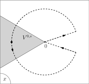
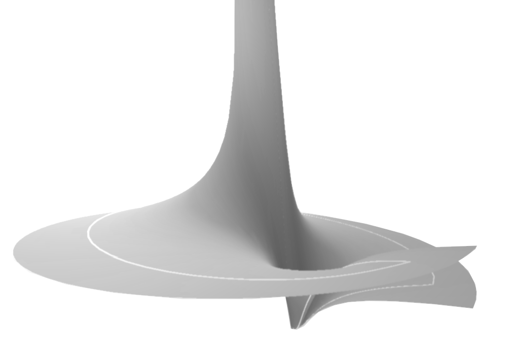
Figure 1.1. An asymptotic cycle, in projection in the $x$-variable (left) and in the leaf (right) when $k=1$.

1.2.5. Temporal normal forms: Section 3

Being given $\mu\notin\mathbb{R}_{\leq 0}$ and $X_{R}$ from the previous step of the construction, we consider some collection $\left(f^{j}\right)_{j\in\nicefrac{{\mathbb{Z}}}{{k\mathbb{Z}}}}$. Using again the Cauchy-Heine transformation, we obtain sectorial functions $T^{j}\in\mathcal{O}\left(\mathcal{V}^{j}\right)$ such that $T^{j+1}-T^{j}=f^{j}\circ H^{j}$. The construction ensures that $X_{R}\cdot T^{j+1}=X_{R}\cdot T^{j}$ and hence the functions $g^{j}=X_{R}\cdot T^{j}$ glue to a holomorphic function $g$ for some $g$ with $g\in x\mathfrak{N}\left\{x,y\right\}$, where we define $\mathfrak{N}\left\{x,y\right\}:=y\mathbb{C}\left[x\right]_{<k}\left\{y\right\}$, the algebra of germs of a holomorphic function of the form

$$\mathfrak{N}\left\{x,y\right\} = \left\{f\in\mathbb{C}\left\{x,y\right\}\,:\,f\left(x,y\right)=\sum_{n>0}f_{n}\left(x\right)y^{n}\,\,,\,f_{n}\in\mathbb{C}\left[x\right]_{<k}\right\}\,.$$

Let $G:=\frac{g}{x}$; by construction $U_{G}X_{R}$ has the desired temporal modulus. The construction yields as a by-product a natural section $\mathcal{S}_{R}$ of the period operator

$$\mathcal{S}_{R}\,:\,\left(h\mathbb{C}\left\{h\right\}\right)^{k} \longrightarrow x\mathfrak{N}\left\{x,y\right\}$$

$$\left(f^{j}\right)_{j\in\nicefrac{{\mathbb{Z}}}{{k\mathbb{Z}}}} \longmapsto g\,.$$

The main difficulty here is to control the size of the domain on which $\mathcal{S}_{R}\left(\left(f^{j}\right)_{j}\right)$ is holomorphic in terms of that of the $f^{j}$.

1.2.6. Explicit computations and algorithms: Section 4

Apart from numerical algorithms we establish in order to prove the Computation Theorem in Section 4.2, we also present a way to perform symbolic calculations in Section 4.1. All these techniques are based on the fact that the orbital and temporal modulus are expressed in terms of the period operator (Remark 2.13) and its natural section. The period is nothing else than an integral of an explicit differential form along a path tangent to the vector field. Yet the key point allowing these computations to be carried out is the fact that when $Z$ is a convergent vector field written in Dulac’s prepared form (4.7) then the correspondence linking the Taylor coefficients of a function and that of its period is block-triangular.

When $Z$ is divergent it is still possible to carry out explicit numerical computations, as will be presented in our upcoming work, although the symbolic side appears more difficult to fathom. This difficulty is well-known to specialists, see for instance the discussion appearing in [7].

1.3. Notations and basic definitions

Throughout the article we use the following notations and conventions:

• We use bold-typed letters to refer to vectors $\mathbf{z}=\left(z_{1},\ldots,z_{n}\right)\in\mathbb{C}^{n}$.

• $\mathbb{C}\left[z\right]_{\leq k}$ is the algebra of polynomials in $z$ of degree at most $k$. By extension $\mathbb{C}\left[z\right]_{<k}$ stands for $\mathbb{C}\left[z\right]_{\leq k-1}$ and so on.

• $\mathbb{C}\left[\left[\mathbf{z}\right]\right]$ is the algebra of formal power series in the (multi)variable $\mathbf{z}$.

• $\mathbb{C}\left\{\mathbf{z}\right\}$ is the algebra of germs of a holomorphic function near $\mathbf{0}$ in the (multi)variable $\mathbf{z}$.

• If $\mathcal{U}$ is a domain of $\mathbb{C}^{n}$ let $\mathcal{O}\left(\mathcal{U}\right)$ denote the algebra of functions holomorphic on $\mathcal{U}$. Then let $\mathcal{O}\left(\mathcal{U}\right)\left\{y\right\}$ denote the set of functions holomorphic on $\mathcal{U}\times r\mathbb{D}$ for sufficiently small $r>0$ ; more precisely, it is the inductive limit of the algebras $\mathcal{O}\left(\mathcal{U}\times r\mathbb{D}\right)$ as $r\to 0$.

• $Z$ is a saddle-node vector field near $\left(0,0\right)$ under Dulac’s prepared form (1.1). The notation $X$ is in general reserved to saddle-node vector fields whose $\frac{\partial}{\partial x}$-component is a function of $x$ only.

• $Z\cdot$ stands for the Lie derivative along $Z$, stably acting on $\mathbb{C}\left[\left[x,y\right]\right]$ and on $\mathbb{C}\left\{x,y\right\}$.

• $\left(k,\mu\right)\in\mathbb{N}_{>0}\times\mathbb{C}\backslash\mathbb{R}_{\leq 0}$ is the formal orbital modulus of $Z$ while $P\in\mathbb{C}\left[x\right]_{\leq k}$ with $P\left(0\right)\neq 0$ is its formal temporal modulus.

• $\mathfrak{N}\left\{x,y\right\}:=y\mathbb{C}\left[x\right]_{<k}\left\{y\right\}$ is the algebra of germs of a holomorphic function of the form

  $$\mathfrak{N}\left\{x,y\right\} = \left\{f\in\mathbb{C}\left\{x,y\right\}\,:\,f\left(x,y\right)=\sum_{n>0}f_{n}\left(x\right)y^{n}\,\,,\,f_{n}\in\mathbb{C}\left[x\right]_{<k}\right\}\,.$$

• $\left(V^{j}\right)_{j\in\nicefrac{{\mathbb{Z}}}{{k\mathbb{Z}}}}$ are the sectors in the $x$-variable which covers $\mathbb{C}_{\neq 0}$, see Definition 2.1 and Figures 2.1, 2.2. From these we construct

  $$V^{j,s} := V^{j}\cap V^{j+1}\,.$$

• If $\mathcal{V}$ is a domain of $\mathbb{C}^{2}$ we define the associated sectors $\mathcal{V}^{j}$ and $\mathcal{V}^{j,s}$ as $\mathcal{V}\cap\left(V^{j}\times\mathbb{C}\right)$ and $\mathcal{V}\cap\left(V^{j,s}\times\mathbb{C}\right)$ respectively, for $j\in\nicefrac{{\mathbb{Z}}}{{k\mathbb{Z}}}$. One kind of domain will be of special interest:

  $$\mathcal{V}_{\rho} := \mathbb{C}\times\rho\mathbb{D}=\left\{\left(x,y\right)\,:\,\left|y\right|<\rho\right\}$$

  for $\rho>0$.

• $X_{R}$ is the vector field associated to some $R\in y\mathbb{C}\left\{x,y\right\}$ by

  $$X_{R} := x^{k+1}\frac{\partial}{\partial x}+y\left(1+\mu x^{k}+xR\right)\frac{\partial}{\partial y}.$$

  It represents one of the normal forms given in Theorem Main Theorem, if $R\in\mathfrak{N}\left\{x,x^{\sigma}y\right\}$. Observe that for $R=0$, we obtain the formal model $X_{0}=x^{k+1}\frac{\partial}{\partial x}+y\left(1+\mu x^{k}\right)\frac{\partial}{\partial y}$.

• $N=\left(N^{j}\right)_{j\in\nicefrac{{\mathbb{Z}}}{{k\mathbb{Z}}}}$ is the collection of sectorial normalizing functions for $X_{R}$, that is functions $N^{j}\in y\mathcal{O}\left(V^{j}\right)\left\{y\right\}$ such that $\left(x,y\exp N^{j}\right)^{*}X_{0}=X_{R}$.

• $H_{N}^{j}\in y\mathcal{O}\left(V^{j}\right)\left\{y\right\},\ j\in\nicefrac{{\mathbb{Z}}}{{k\mathbb{Z}}}$, are the sectorial first-integral associated to $X_{R}$ (Definition 2.3):

  $$H_{N}^{j}\left(x,y\right) := y\,e^{2i\pi\mu j/k}\exp\left(\frac{x^{-k}}{k}-\mu\log x+N^{j}\left(x,y\right)\right)\,.$$

  Here the branch of the logarithm is chosen according to the sector, i.e. such that $\left|\arg x-j\frac{2\pi}{k}\right|\leq\frac{\pi}{k}+\beta$ for small $x$.

• $\mathcal{T}_{R}$ is the period operator associated to $X_{R}$ (see Definition 1.5) and $\mathcal{S}_{R}$ its natural section (see Corollary 3.1)

  $$\mathcal{T}_{R}\,:\,x^{k+1}\mathbb{C}\left\{x\right\}+y\mathbb{C}\left\{x,y\right\} \longrightarrow \left(h\mathbb{C}\left\{h\right\}\right)^{k}$$

  $$\mathcal{S}_{R}\,:\,\left(h\mathbb{C}\left\{h\right\}\right)^{k} \longrightarrow x\mathfrak{N}\left\{x,y\right\}\,.$$

• $\mathcal{M}\left(Z\right)=\left(\mu,P\right)\oplus\left(\varphi^{j},f^{j}\right)_{j\in\nicefrac{{\mathbb{Z}}}{{k\mathbb{Z}}}}$ is the complete analytic modulus of $Z$. If $Z=U_{G}X_{R}$ is the associated normal form then

  $$\left(\varphi^{j},f^{j}\right)_{j\in\nicefrac{{\mathbb{Z}}}{{k\mathbb{Z}}}} = \mathcal{T}_{R}\left(-xR\right)\oplus\mathcal{T}_{R}\left(\frac{1}{U_{G}}-\frac{1}{P}\right)\,.$$

We introduce also some Banach spaces and norms.

Definition 1.6.

Let $\mathcal{D}\subset\mathbb{C}^{n}$ be a domain containing $\mathbf{0}$ equipped with the coordinate $\mathbf{z}=\left(z_{1},\cdots,z_{n}\right)$.

1. We define the Banach space $\mathcal{B}\left(\mathcal{D}\right)$ of functions bounded and holomorphic on $\mathcal{D}$ with values in $\mathbb{C}$ equipped with the norm:

   $$\left|\left|f\right|\right|_{\mathcal{D}} := \sup_{\mathbf{z}\in\mathcal{D}}\left|f\left(\mathbf{z}\right)\right|\,.$$

2. We define the Banach space $\mathcal{B}^{\prime}\left(\mathcal{D}\right)$ of functions holomorphic on $\mathcal{D}$, vanishing along $\left\{z_{n}=0\right\}$, equipped with the norm

   $$\left|\left|f\right|\right|_{\mathcal{D}}^{\prime} := \sup_{\mathbf{z}\in\mathcal{D}}\frac{\left|f\left(\mathbf{z}\right)\right|}{\left|z_{n}\right|}\,.$$

   Notice that

   $$\left|\left|f\right|\right|_{\mathcal{D}}^{\prime} \leq \left|\left|\frac{\partial f}{\partial z_{n}}\right|\right|_{\mathcal{D}}$$

   when $\frac{\partial f}{\partial z_{n}}\in\mathcal{B}\left(\mathcal{D}\right)$.

3. For a finite collection $\mathcal{D}:=\left(\mathcal{D}_{j}\right)_{j}$,let $\mathcal{B}\left(\mathcal{D}\right)$denote the Banach space $\prod_{j}\mathcal{B}\left(\mathcal{D}_{j}\right)$ equipped with the norm

   $$\left|\left|\left(f_{j}\right)_{j}\right|\right|_{\mathcal{D}} := \max_{j}\left|\left|f_{j}\right|\right|_{\mathcal{D}_{j}}\,.$$

   The analogous definition is used for the space $\mathcal{B}^{\prime}\left(\mathcal{D}\right)$.

In general we omit to indicate the dependence of the norm on the domain when the context is not ambiguous.

2. Orbital normal forms

Recall that in the following section $\mu$ is a non-zero, non-negative complex number.

2.1. Sectorial decomposition and first-integrals

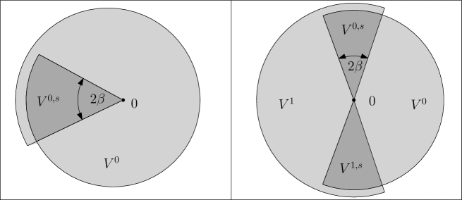
Figure 2.1. Sectors near $0$ in the case $k=1$ (left) along with the case $k=2$ (right)

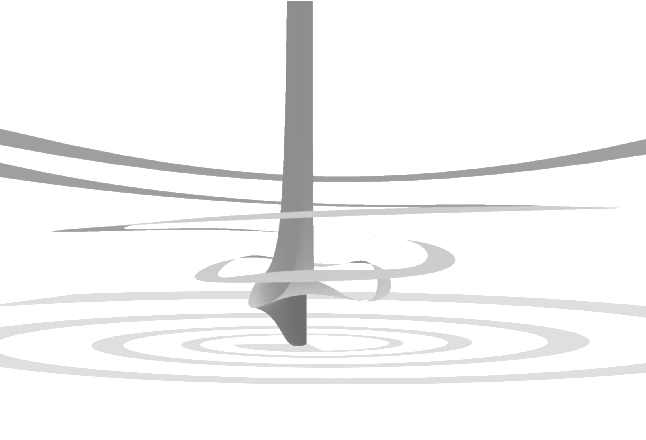
Figure 2.2. The sector $V^{0}$ in the $x$-variable (top) and the absolute value of a sectorial leaf of the formal model over it (bottom) for $k=3$ and $\mu=-\frac{1}{10}\left(1+\textrm{i}\right)$.

We fix once and for all a real number

$$0 <\beta< \frac{\pi}{2k}.$$

Definition 2.1.

This definition should be read with the Figures 2.1 and 2.2 in mind.

1. The sectorial decomposition of the $x$-variable is the collection of $k$ sector-like domains $V^{j}$ defined as the union of

   • a standard sector of $r\mathbb{D}$

     $$\left\{x\,:\,\left|\arg x-\theta^{j}\right|<\frac{\pi}{k}+\beta\,\,\,\textrm{and}\,\,\,0<\left|x\right|<r\right\} \,\,\,,\,j\in\nicefrac{{\mathbb{Z}}}{{k\mathbb{Z}}}$$

     where $\theta^{j}:=j\frac{2\pi}{k}$

   • a spiraling sector, bounded by two spirals

     $$S^{j,\pm} :=r\exp\left(\textrm{i}\theta^{j}\pm\textrm{i}\frac{\pi}{k}\pm\textrm{i}\beta\right)\exp\left(\left(1+\textrm{i}\nu\right)\mathbb{R}_{\geq 0}\right) \,\,\,,\,j\in\nicefrac{{\mathbb{Z}}}{{k\mathbb{Z}}}$$

     where $\nu\in\mathbb{R}$ is chosen (once and for all) in such a way that

     (2.1) $$\Re\left(\mu\right) > \nu\Im\left(\mu\right)\,.$$

     In particular when $\Re\left(\mu\right)>0$ we can take $\nu:=0$ and the sector $V^{j}$ coincides with a standard sector of infinite radius.

   Notice that $\bigcup_{j\in\nicefrac{{\mathbb{Z}}}{{k\mathbb{Z}}}}V^{j}=\mathbb{C}\backslash\left\{0\right\}$.

2. We denote by $\Gamma^{j,\pm}$ the two connected components of $\partial V^{j}$, consisting of the concatenation of the segment $I^{j,\pm}:=]0,r\exp\left(\textrm{i}\theta^{j}\pm\textrm{i}\frac{\pi}{k}\pm\textrm{i}\beta\right)]$ and the spiral $S^{j,\pm}$.

3. We define the saddle-part of $V^{j}$ as

   $$V^{j,s} := V^{j}\cap V^{j+1}\,.$$

4. For any domain $\mathcal{V}\subset\mathbb{C}^{2}$ containing $\left\{y=0\right\}$ we define the sectorial decomposition of $\mathcal{V}$ by

   $$\mathcal{V}^{j} := \mathcal{V}\cap\left(V^{j}\times\mathbb{C}\right)\,\,\,\,\,,\,j\in\nicefrac{{\mathbb{Z}}}{{k\mathbb{Z}}}$$

   $$\mathcal{V}^{j,s} := \mathcal{V}\cap\left(V^{j,s}\times\mathbb{C}\right)\,\,\,\,\,,\,j\in\nicefrac{{\mathbb{Z}}}{{k\mathbb{Z}}}$$

Remark 2.2.

In the case $k=1$ there is a slight problem in the definition of $V^{0}$. We make the convention that $V^{0}$, near $0$, is a sector of aperture greater than $2\pi$ which overlaps with itself above $\mathbb{R}_{<0}$ without gluing (see Figure 2.1). Let $V^{0,s}$ denote this overlap in the case $k=1$.

Definition 2.3.

Let $\mathcal{V}\subset\mathbb{C}^{2}$ be a domain containing $\left\{y=0\right\}$.

For every collection $N:=\left(N^{j}\right)_{j\in\nicefrac{{\mathbb{Z}}}{{k\mathbb{Z}}}}$in $\mathcal{B}\left(\left(\mathcal{V}^{j}\right)_{j}\right)$ we define the collection $\left(H_{N}^{j}\right)_{j\in\nicefrac{{\mathbb{Z}}}{{k\mathbb{Z}}}}$ of $k$ functions by

$$H_{N}^{j}\left(x,y\right) := y\,e^{2\textrm{i}\pi j\mu/k}\exp\left(\frac{1}{kx^{k}}-\mu\log x+N^{j}\left(x,y\right)\right)\,,$$

where we choose the determination of the logarithm such that $\left|\arg x-j\frac{2\pi}{k}\right|\leq\frac{\pi}{k}+\beta$ for small $x\in V^{j}$ and such that it is an analytic function in this «spiraling sector». In this way, the value of $H_{N}^{j}(x,y)$ indeed only depends upon the class of $j$ modulo $k$.

This collection is called the sectorial first-integrals associated to $N$.

2.2. Admissible domains and the refined Cauchy-Heine transform

Definition 2.4.

Let $\rho\in]0,+\infty]$ be given.

1. We define the domain

   $$\mathcal{V}_{\rho} := \mathbb{C}\times\rho\mathbb{D}=\left\{\left(x,y\right)\in\mathbb{C}^{2}\,:\,\left|y\right|<\rho\right\}\,,$$

   which is a neighborhood of $\left\{y=0\right\}$.

2. A collection $\Delta=\left(\Delta^{j}\right)_{j\in\nicefrac{{\mathbb{Z}}}{{k\mathbb{Z}}}}$ of $k$ domains of $\mathbb{C}$ containing $0$ will be called admissible.

3. We say that a couple $\left(\rho,N\right)$ with $N=\left(N^{j}\right)\in\mathcal{B}\left(\left(\mathcal{V}_{\rho}^{j}\right)_{j\in\nicefrac{{\mathbb{Z}}}{{k\mathbb{Z}}}}\right)$ is adapted to an admissible collection $\Delta$ if $H_{N}^{j}\left(\mathcal{V}_{\rho}^{j,s}\right)\subset\Delta^{j}$ for each $j\in\nicefrac{{\mathbb{Z}}}{{k\mathbb{Z}}}$.

The next result is the basis of our construction.

Theorem 2.5.

Consider some admissible collection $\Delta$ and some $\left(\rho,N\right)$ adapted to $\Delta$ with $\rho<+\infty$. Take any collection $f=\left(f^{j}\right)_{j\in\nicefrac{{\mathbb{Z}}}{{k\mathbb{Z}}}}\in\mathcal{B}^{\prime}\left(\Delta\right)$ and define the collection $\Sigma=\left(\Sigma^{j}\right)_{j\in\nicefrac{{\mathbb{Z}}}{{k\mathbb{Z}}}}$ by

$$\Sigma^{j}\left(x,y\right) := \frac{x}{2\textrm{i}\pi}\sum_{\ell\neq j+1}\int_{\Gamma^{\ell-}}\frac{f^{\ell}\left(H_{N}^{\ell}\left(z,y\right)\right)}{z\left(z-x\right)}\textrm{d}z+\frac{x}{2\textrm{i}\pi}\int_{\Gamma^{j+}}\frac{f^{j}\left(H_{N}^{j}\left(z,y\right)\right)}{z\left(z-x\right)}\textrm{d}z,\ \ (x,y)\in\mathcal{V}_{\rho}^{j},$$

where the paths were described in Definition 2.1. Here integrals over $\Gamma^{\ell\pm}$ are more precisely integrals in $V^{\ell}$over paths arbitrarily close to $\Gamma^{\ell\pm}$. The following properties hold.

1. $\Sigma^{j}\in\mathcal{B}\left(\mathcal{V}^{j}\right)$.

2. For all $j\in\nicefrac{{\mathbb{Z}}}{{k\mathbb{Z}}}$ we have

   $$\Sigma^{j+1}-\Sigma^{j} = f^{j}\circ H_{N}^{j}$$

   on $\mathcal{V}_{\rho}^{j,s}$.

3. For every $j\in\nicefrac{{\mathbb{Z}}}{{k\mathbb{Z}}}$

   $$\lim_{x\to 0}\Sigma^{j}\left(x,y\right) = 0$$

   locally uniformly in $y\in$$\rho\mathbb{D}$.

4. Any other collection $\left(\tilde{\Sigma}^{j}\right)_{j\in\nicefrac{{\mathbb{Z}}}{{k\mathbb{Z}}}}\in\mathcal{B}\left(\left(\mathcal{V}_{\rho}^{j}\right)_{j\in\nicefrac{{\mathbb{Z}}}{{k\mathbb{Z}}}}\right)$ satisfying (1) and (2) differs from $\Sigma$ by the component-wise addition of a single holomorphic function $y\mapsto F\left(y\right)$ in $\mathcal{B}\left(\rho\mathbb{D}\right)$.

5. One has the estimates

   1. $$\left|\left|\Sigma\right|\right| \leq \rho K\left|\left|f\right|\right|^{\prime}e^{\left|\left|N\right|\right|}$$

   2. $$\left|\left|y\frac{\partial\Sigma}{\partial y}\right|\right| \leq \rho K\left|\left|f^{\prime}\right|\right|e^{\left|\left|N\right|\right|}\left(1+\left|\left|y\frac{\partial N}{\partial y}\right|\right|\right)$$

   3. $$\left|\left|x\frac{\partial\Sigma}{\partial x}\right|\right| \leq \rho K\left|\left|f^{\prime}\right|\right|e^{\left|\left|N\right|\right|}\left(1+\left|\left|x\frac{\partial N}{\partial x}\right|\right|\right)$$

      with some constant $K>0$ depending only on $k$, $\mu$, $\nu$, $\beta$ and $r$.

Remark 2.6.

A value for $K$ is given in the proof, but not very explicitly.

Definition 2.7.

Under the hypothesis of the theorem, we let the refined Cauchy-Heine transform of $f$, associated to $N$, denote the collection of functions $\Sigma\left(N,f\right):=\left(\Sigma^{j}\right)_{j\in\nicefrac{{\mathbb{Z}}}{{k\mathbb{Z}}}}$ defined by the previous theorem. We choose this set of functions satisfying (2) because they are <<normalized>>: they tend to $0$ as $V^{j}\ni x\to 0$.

Let us now give a proof to Theorem 2.5.

Proof.

In order to prove the holomorphy of $\Sigma^{j}$ and as a first step to establish the estimates (5), we only consider the case of the integral along $\Gamma^{j,+}$. For the sake of clarity we omit, wherever not confusing, to indicate the indexes $j$, $N$ and $+$.

By the above Definitions 1.6 and 2.3, one has

(2.2) $$\left|x\frac{f\left(H\left(z,y\right)\right)}{z(z-x)}\textrm{d}z\right| \leq \left|\left|f\right|\right|^{\prime}\left|xH\left(z,y\right)\frac{\textrm{d}z}{z(z-x)}\right|$$

(2.3) $$\leq \rho A\left|\left|f\right|\right|^{\prime}e^{\left|\left|N\right|\right|}q\left(x\right)\left|z^{-\mu-1}\exp\frac{z^{-k}}{k}\right|\left|\textrm{d}z\right|$$

where $q\left(x\right)=\sup\left\{\frac{|x|}{|z-x|}\text{~}:\text{~}z\in\Gamma\right\}$ and $A=e^{2\pi\left|\mu\right|}$. The first thing to establish is that the improper integrals in the construction of $\Sigma$ are absolutely convergent. Using the notation introduced in Definition 2.1, we have for $z\in I$

$$z = x_{*}t\,\,\,,\,t\in\left[0,1\right]$$

$$\left|\textrm{d}z\right| = r\textrm{d}t$$

where

$$x_{*} := r\exp\left(\textrm{i}\frac{\pi}{k}\left(2j+1\right)+\textrm{i}\beta\right)\,,$$

while for $z\in S$

$$z = x_{*}\exp\left(\left(1+\textrm{i}\nu\right)t\right)\,\,\,,\,t\geq 0$$

$$\left|\textrm{d}z\right| = \left|1+\textrm{i}\nu\right|\left|z\right|\textrm{d}t\,.$$

For $z\in I$ we have $\arg\left(z^{k}\right)=\pi+k\beta$ and therefore

$$\left|z^{-\mu-1}\exp\left(\frac{z^{-k}}{k}\right)\textrm{d}z\right| \leq \left|x_{*}^{-\mu-1}\right|t^{-\Re\left(\mu\right)-1}\exp\left(-r^{-k}\cos\left(k\beta\right)t^{-k}/k\right)\textrm{d}t$$

is integrable on $\left[0,1\right]$. For $z$ is on $S$ we have $\left|z^{-\mu-1}\right|=\left|x_{*}^{-\mu-1}\right|e^{\alpha t}$ with

$$\alpha :=-\Re\left(\mbox{$\left(\mu+1\right)\left(1+i\nu\right)$}\right)= -\Re\left(\mu\right)-1+\nu\Im\left(\mu\right)<-1$$

(see Definition 2.1) and therefore

$$\left|z^{-\mu-1}\exp\left(\frac{z^{-k}}{k}\right)\textrm{d}z\right| \leq \left|1+\nu\textrm{i}\right|\exp\frac{r^{-k}}{k}\left|x_{*}^{-\mu}\right|e^{\left(\alpha+1\right)t}\textrm{d}t$$

is also integrable on $[0,+\infty[$. Hence

$$\left|\frac{x}{2\textrm{i}\pi}\int_{\Gamma}\frac{f\left(H\left(z,y\right)\right)}{z\left(z-x\right)}\textrm{d}z\right|\leq\rho AL\left|\left|f\right|\right|^{\prime}e^{\left|\left|N\right|\right|}q\left(x\right),$$

where $L=\frac{1}{2\pi}\int_{\Gamma}\left|z^{-\mu-1}\exp\frac{z^{-k}}{k}\right|\left|\textrm{d}z\right|.$ In the case of $\mu$ with negative real part, it is crucial to use the spiral shape of the paths near $\infty$ as required by (2.1) of Definition 2.1.

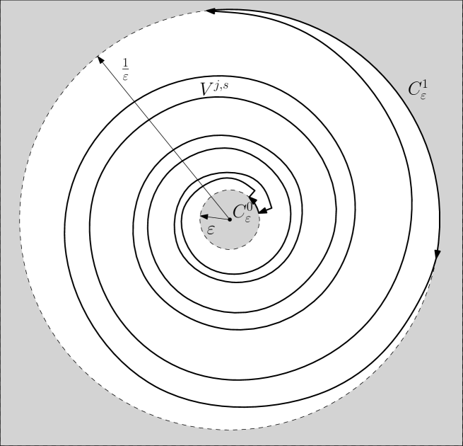
Figure 2.3.

By choosing the paths of integration sufficiently close to the boundaries of the sectors, we obtain that $\Sigma^{j}$ is an analytic function on $\mathcal{V}_{\rho}^{j}$. The boundedness of $\Sigma$ will be shown later; only then the proof of (1) is complete.

Claim (2) is obtained by Cauchy’s formula. For $\varepsilon>0$ small enough, we define the contour $\mathcal{C}_{\varepsilon}$ as in Figure 2.3. It is positively oriented and consists of:

• the arc $C_{\varepsilon}^{0}$ of the circle $\left\{\left|z\right|=\varepsilon\right\}$ between $\Gamma^{j,+}$ and $\Gamma^{j+1,-}$,

• the curve $\Gamma^{j+1,-}\cap\left\{\varepsilon\leq\left|z\right|\leq\frac{1}{\varepsilon}\right\}$,

• the arc $C_{\varepsilon}^{1}$ of the circle $\left\{\left|z\right|=\frac{1}{\varepsilon}\right\}$ between $\Gamma^{j,+}$ and $\Gamma^{j+1,-}$,

• the curve $\Gamma^{j,+}\cap\left\{\varepsilon\leq\left|z\right|\leq\frac{1}{\varepsilon}\right\}$, .

Therefore whenever $x\in V^{j,s}$, $\varepsilon<\left|x\right|<\frac{1}{\varepsilon},$ we have

$$\frac{1}{2\textrm{i}\pi}\int_{\mathcal{C}_{\varepsilon}}\frac{f^{j}\left(H_{N}^{j}\left(z,y\right)\right)}{z\left(z-x\right)}\textrm{d}z = \frac{f^{j}\left(H_{N}^{j}\left(x,y\right)\right)}{x}\,.$$

Taking the limit as $\varepsilon\to 0$ yields that

(2.4) $$\frac{x}{2\textrm{i}\pi}\int_{\Gamma^{j+1,-}}\frac{f^{j}\left(H_{N}^{j}\left(z,y\right)\right)}{z\left(z-x\right)}\textrm{d}z-\frac{x}{2\textrm{i}\pi}\int_{\Gamma^{j+}}\frac{f^{j}\left(H_{N}^{j}\left(z,y\right)\right)}{z\left(z-x\right)}\textrm{d}z=f^{j}\left(H_{N}^{j}\left(x,y\right)\right)$$

because the integrals on $C_{\varepsilon}^{0}$ and $C_{\varepsilon}^{1}$ tend to $0$. Indeed, for values of $\varepsilon$ less than $\min\left(r,\frac{\left|x\right|}{2}\right)$, if $z\in C_{\varepsilon}^{0}$, then we have $\left|\arg z-\left(2j+1\right)\frac{\pi}{k}\right|<\beta$ and $\left|z\left(z-x\right)\right|\geq\varepsilon\left|\frac{x}{2}\right|$ . Therefore

$$\int_{C_{\varepsilon}^{0}}\left|\frac{xz^{-\mu-1}}{z-x}\exp\left(\frac{z^{-k}}{k}\right)\textrm{d}z\right| \leq 4\beta\varepsilon^{-\Re\left(\mu\right)}e^{2\pi\left|\mu\right|}\exp\left(-\frac{\varepsilon^{-k}}{k}\cos\left(k\beta\right)\right)\,.$$

If $z\in C_{\varepsilon}^{1}$ we still have $\left|z-x\right|\geq\left|x\right|$ and therefore

$$\int_{C_{\varepsilon}^{1}}\left|\frac{xz^{-\mu-1}}{z-x}\exp\left(\frac{z^{-k}}{k}\right)\textrm{d}z\right| \leq 2\beta\,r^{-\nu\Im\left(\mu\right)}e^{2\pi\left|\mu\right|}\varepsilon^{-\alpha-1}\exp\left(\frac{\varepsilon^{k}}{k}\right)\,.$$

In a similar way, we show that

$$\frac{x}{2\textrm{i}\pi}\int_{\Gamma^{j+1,+}}\frac{f^{j+1}\left(H_{N}^{j+1}\left(z,y\right)\right)}{z\left(z-x\right)}\textrm{d}z=\frac{x}{2\textrm{i}\pi}\int_{\Gamma^{j+2,-}}\frac{f^{j+1}\left(H_{N}^{j+1}\left(z,y\right)\right)}{z\left(z-x\right)}$$

for $\left(x,y\right)\in\mathcal{V}^{j+1,s}$. This completes the proof of (2).

Next we show (5)(a) (and at the same time the boundedness part of (1)). For that purpose, we first consider the subset $W^{j}$ of $V^{j}$ containing all $x$ such that $xe^{\textrm{i}s}\in V^{j}$ for real $s,$ $0\leq s\leq\beta/2.$ Then $q_{j}\left(x\right)\leq 1/\sin\left(\beta/2\right)$ if $\left|x\right|$ is small whereas $1/q_{j}\left(x\right)$ is bounded below by the distance of the point $e^{\textrm{i}\beta/2}$ to the spiral $\exp\left(\left(1+\textrm{i}\nu\right)\mathbb{R}\right)$ for large $\left|x\right|.$ As $q_{j}$ is a continuous function, this implies that it is bounded on $W^{j}$. Let $Q$ denote some bound. Thus we have shown that

$$\left|\frac{x}{2\textrm{i}\pi}\int_{\Gamma^{j,+}}\frac{f^{j}\left(H_{N}^{j}\left(z,y\right)\right)}{z\left(z-x\right)}\textrm{d}z\right|\leq\rho ALQ\left|\left|f\right|\right|^{\prime}e^{\left|\left|N\right|\right|}$$

for $x\in W^{j}$ and $\left|y\right|\leq\rho$. For $x\in V^{j}\setminus W^{j}$, we use (2.4) and estimate the integral over $\Gamma^{j+1,-}$ in the same way. This yields

$$\left|\frac{x}{2\textrm{i}\pi}\int_{\Gamma^{j,+}}\frac{f^{j}\left(H_{N}^{j}\left(z,y\right)\right)}{z\left(z-x\right)}\textrm{d}z\right|\leq\rho A(LQ+M)\left|\left|f\right|\right|^{\prime}e^{\left|\left|N\right|\right|}$$

for $x\in V^{j},\left|y\right|\leq\rho$, where $M$ denotes the supremum of $\left|x^{-\mu-1}\exp\frac{x^{-k}}{k}\right|$ on $V^{j}.$ The remaining integrals in the definition of $\Sigma^{j}$ are treated similarly. This yields (5)(a).

From the above estimates, we can also deduce (5)(b): since

$$y\frac{\partial H}{\partial y}\left(x,y\right)=H\left(x,y\right)\left(1+y\frac{\partial N}{\partial y}\left(x,y\right)\right)$$

we use

$$\left|x\frac{f^{\prime}\left(H\left(z,y\right)\right)}{z(z-x)}y\frac{\partial H}{\partial y}\left(z,y\right)dz\right| \leq \rho A\left|\left|f^{\prime}\right|\right|e^{\left|\left|N\right|\right|}\left|\left|1+y\frac{\partial N}{\partial y}\right|\right|q\left(x\right)\left|z^{-\mu-1}\exp\frac{z^{-k}}{k}\right|\left|\textrm{d}z\right|$$

instead of (2.2).

For (5)(c), observe that

$$x\frac{\partial\Sigma^{j}}{\partial x}\left(x,y\right)=\Sigma^{j}(x,y)+\frac{x^{2}}{2\textrm{i}\pi}\sum_{\ell\neq j+1}\int_{\Gamma^{\ell-}}\frac{f^{\ell}\left(H_{N}^{\ell}\left(z,y\right)\right)}{z\left(z-x\right)^{2}}\textrm{d}z+\frac{x^{2}}{2\textrm{i}\pi}\int_{\Gamma^{j+}}\frac{f^{j}\left(H_{N}^{j}\left(z,y\right)\right)}{z\left(z-x\right)^{2}}\textrm{d}z,\ \ (x,y)\in\mathcal{V}_{\rho}^{j}.$$

We estimate the new integrals similarly to the beginning using

$$\left|x^{2}\frac{f\left(H\left(z,y\right)\right)}{z(z-x)^{2}}\textrm{d}z\right|\leq\rho A\left|\left|f\right|\right|^{\prime}e^{\left|\left|N\right|\right|}q\left(x\right)^{2}\left|z^{-\mu-1}\exp\frac{z^{-k}}{k}\right|\left|\textrm{d}z\right|$$

instead of (2.2). For $x$ close to $\Gamma^{j,+}$(or to $\Gamma^{j-1,-}$) we have to use Cauchy’s formula similarly to (2.4), but obtain on the right hand side $x^{2}\frac{\partial}{\partial x}\left(\frac{1}{x}f^{j}\left(H_{N}^{j}\left(x,y\right)\right)\right)$. This requires an estimate of

$$x\frac{\partial}{\partial x}\left(f^{j}\left(H_{N}^{j}\left(x,y,\right)\right)\right)=\frac{\textrm{d}f^{j}}{\textrm{d}h}\left(H_{N}^{j}\left(x,y\right)\right)H_{N}^{j}\left(x,y\right)\left(-x^{-k}-\mu+x\frac{\partial N}{\partial x}\right)$$

on $V^{j}$. This is done analogously to the proof of (5)(a) and yields the desired result.

For (3), we use instead of (2.2)

$$\left|\frac{f\left(H\left(z,y\right)\right)}{z(z-x)}\textrm{d}z\right|\leq\left|\left|f\right|\right|^{\prime}\left|H\left(z,y\right)\frac{\textrm{d}z}{z(z-x)}\right|\leq\rho A\left|\left|f\right|\right|^{\prime}e^{\left|\left|N\right|\right|}\tilde{q}\left(x\right)\left|z^{-\mu-2}\exp\frac{z^{-k}}{k}\right|\left|\textrm{d}z\right|$$

where $\tilde{q}\left(x\right)=\sup\left\{\frac{|z|}{|z-x|}\mid z\in\Gamma\right\}.$ This yields that $\left|\Sigma^{j}\left(x,y\right)\right|\leq\left|x\right|\rho\tilde{K}\left|\left|f\right|\right|^{\prime}e^{\left|\left|N\right|\right|}$ with some constant $\tilde{K}$ determined in a way analogous to $K$ and hence (3).

Point (4) is a consequence of the fact that the consecutive differences of components of $\tilde{\Sigma}$ and $\Sigma$ agree hence

$$\tilde{\Sigma}^{j}\left(x,y\right)-\Sigma^{j}\left(x,y\right) =: \delta\left(x,y\right)$$

defines a bounded, holomorphic function on $\mathbb{C}_{\neq 0}\times\rho\mathbb{D}$. Riemann’s Theorem on removable singularities tells us that $\delta$ can be extended holomorphically to a bounded function on $\mathbb{C}\times\rho\mathbb{D}$, which must be a function of $y$ only according to Liouville’s theorem. ∎

2.3. Construction of a vector field with given sectorial transition maps

Here we want to find a vector field $X_{R}$ with prescribed transition maps between sectorial first-integrals. This construction is the core of the proof for the orbital normal form reduction.

Proposition 2.8.

Let an admissible collection $\Delta$ and a collection $\varphi\in\mathcal{B}^{\prime}\left(\Delta\right)$ be given. Then there exists $\left(\rho,N\right)$ adapted to $\Delta$ such that

1. $$H_{N}^{j+1} = H_{N}^{j}\exp\left(\frac{2\textrm{i}\pi\mu}{k}+\varphi^{j}\left(H_{N}^{j}\right)\right)\,,$$

2. $$\left|\left|y\frac{\partial N}{\partial y}\right|\right| < 1\,,\left|\left|x\frac{\partial N}{\partial x}\right|\right|<1.$$

Remark 2.9.

A value for $\rho$ is given in the proof.

This proposition relies on a general convergence result for sequences in the space $\mathcal{B}\left(\Delta\right)$, which we have not been able to find in the literature but should come in handy in many problems where the most direct approach is formal.

Lemma 2.10.

Let $\Delta$ be a domain in $\mathbb{C}^{m}$ and consider a bounded sequence $\left(f_{p}\right)_{p\in\mathbb{N}}$ of $\mathcal{B}\left(\Delta\right)$ satisfying the additional property that there exists some point $\mathbf{z}_{0}\in\Delta$ such that the corresponding sequence of Taylor series $\left(T_{p}\right)_{p\in\mathbb{N}}$ at $\mathbf{z}_{0}$ is convergent in $\mathbb{C}\left[\left[\mathbf{z}-\mathbf{z}_{0}\right]\right]$ equipped with the projective topology. Then $\left(f_{p}\right)_{p}$ converges uniformly on compact sets of $\Delta$ towards some $f_{\infty}\in\mathcal{B}\left(\Delta\right)$.

Remark 2.11.

1. The convergence of the sequence of Taylor series $\left(T_{p}\right)_{p\in\mathbb{N}}=\left(\sum_{\mathbf{n}\geq 0}a_{\mathbf{n}}^{\left(p\right)}\left(\mathbf{z}-\mathbf{z}_{0}\right)^{\mathbf{n}}\right)_{p\in\mathbb{N}}$ for the projective topology is equivalent to that of each sequence $\left(a_{\mathbf{n}}^{\left(p\right)}\right)_{p\in\mathbb{N}}$ in $\mathbb{C}$. This is particularly the case when $\left(T_{p}\right)_{p\in\mathbb{N}}$ converges for the Krull topology

2. The convergence might not be uniform on $\Delta$: as an example take $\Delta:=\left\{z\in\mathbb{C}\,:\,\left|z\right|<1\right\}$ and $f_{p}\left(z\right):=z^{p}$.

Proof.

Let $\mathcal{O}\left(\Delta\right)$ denote the space of functions holomorphic on $\Delta$, equipped with the topology of uniform convergence on compact subsets of $\Delta$, which is a Montel space. If the sequence $\left(f_{p}\right)_{p}$ is bounded in $\mathcal{B}\left(\Delta\right)$ it is also bounded in $\mathcal{O}\left(\Delta\right)$. Consequently, there exists a convergent subsequence $\left(f_{p_{j}}\right)_{j\in\mathbb{N}}$ in $\mathcal{O}\left(\Delta\right)$; call $f_{\infty}$ its limiting value. Now Cauchy’s integral formula and the uniform convergence $\left(f_{p_{j}}\right)_{j}\to f_{\infty}$ on a small compact polydisc around $\mathbf{z}_{0}$ imply that the Taylor series of $f_{\infty}$ at $\mathbf{z}_{0}$ coincides with the limiting power series $\lim_{p}T_{p}$. This argument, together with the identity theorem on the connected open set $\Delta$, is sufficient to prove that any other subsequence of $\left(f_{p}\right)_{p}$ converges toward the same function $f_{\infty}$. This implies the convergence $\left(f_{p}\right)_{p}\to f_{\infty}$ in $\mathcal{O}\left(\Delta\right)$. The boundedness of the sequence $\left(f_{p}\right)_{p}$in $\mathcal{B}\left(\Delta\right)$ implies that $f_{\infty}$ is bounded by the same constant on each compact subset of $\Delta$, i.e. it belongs to $\mathcal{B}\left(\Delta\right)$. ∎

We now give a proof of Proposition 2.8.

Proof.

We recursively define the sequence $\left(N_{n}\right)_{n\in\mathbb{N}}$: starting with $N_{0}:=0$ we put

(2.5) $$N_{n+1} := \Sigma\left(N_{n},\varphi\right),\ n\geq 0$$

using the refined Cauchy-Heine transform of Definition 2.7 and Theorem 2.5. Then we show it converges in a convenient Banach space. For the sake of clarity we omit the superscript $j$ whenever not confusing, and write $H_{n}$ instead of $H_{N_{n}}$.

We can assume that all $\varphi^{j}$ are holomorphic and have bounded derivatives on some disc $\eta\mathbb{D}\subset\bigcap_{j\in\nicefrac{{\mathbb{Z}}}{{k\mathbb{Z}}}}\Delta_{j}$. Then we choose

$$\rho \leq \frac{\eta}{M}e^{-\frac{\eta}{M}K\left|\left|\varphi^{\prime}\right|\right|_{\eta\mathbb{D}}}$$

where

$$M=M\left(k,\mu,\nu,\beta\right) :=e^{2\pi\left|\mu\right|} \sup_{z\in V^{j,s}}\left|z^{-\mu}\exp\frac{z^{-k}}{k}\right|$$

and $K$ is the constant appearing in Theorem 2.5. We need to ensure that

(2.6) $$\left(\forall n\in\mathbb{N}\right)\,\left(\forall y\in\rho\mathbb{D}\right)\,\left(\forall z\in V^{j,s}\right) \left|H_{n}\left(z,y\right)\right|\leq\eta\,.$$

By construction of $H_{n}$ we have for $\left(z,y\right)\in\mathcal{V}_{\rho}^{j}$

$$\left|H_{n}\left(z,y\right)\right| \leq \rho e^{2\pi\left|\mu\right|}\left|z^{-\mu}\exp\frac{z^{-k}}{k}\right|e^{\left|\left|N_{n}\right|\right|}\,.$$

Therefore if for some $n\in\mathbb{N}$ we have$\left|\left|N_{n}\right|\right|\leq\frac{2\pi}{M}\eta K\left|\left|\varphi^{\prime}\right|\right|_{\eta\mathbb{D}}$ then we first find that

$$\left|H_{n}\left(z,y\right)\right| \leq \rho M\exp\left(\frac{\eta}{M}K\left|\left|\varphi^{\prime}\right|\right|_{\eta\mathbb{D}}\right)=\eta,$$

i.e. $\left(\rho,N_{n}\right)$ is adapted to $\Delta$ and then, using Theorem 2.5 (5)(a), we obtain

$$\left|\left|N_{n+1}\right|\right| \leq \rho K\left|\left|\varphi\right|\right|_{\eta\mathbb{D}}^{\prime}\exp\left|\left|N_{n}\right|\right|$$

$$\leq \rho K\left|\left|\varphi^{\prime}\right|\right|_{\eta\mathbb{D}}\exp\left|\left|N_{n}\right|\right|$$

$$\leq \frac{\eta}{M}K\left|\left|\varphi^{\prime}\right|\right|_{\eta\mathbb{D}}\,.$$

These estimates show by induction on $n$ that, with the above choice of $\rho$, the relation (2.5) defines a bounded sequence $\left(N_{n}\right)_{n}\subset\mathcal{B}\left(\mathcal{V}_{\rho}^{j}\right)$. It is then sufficient to show that the sequence $\left(N_{n}\right)_{n}$ converges for the Krull topology on $\mathcal{B}\left(V^{j}\right)\left[\left[y\right]\right]$ to obtain its convergence towards an element $N$ of the Banach space $\mathcal{B}\left(\mathcal{V}_{\rho}^{j}\right)$ (use Lemma 2.10). By construction this limit is a fixed point of the operator $N\mapsto\Sigma\left(N,\varphi\right)$ (as it is continuous for the compact uniform convergence) and therefore $N^{j+1}-N^{j}=\varphi^{j}\left(H_{N}^{j}\right)$, according to Theorem 2.5. As an immediate consequence we obtain

$$\frac{H_{N}^{j+1}}{H_{N}^{j}} = \exp\left(\frac{2\textrm{i}\pi\mu}{k}+N^{j+1}-N^{j}\right)=\exp\left(\frac{2\textrm{i}\pi\mu}{k}+\varphi^{j}\left(H_{N}^{j}\right)\right)$$

and thus we proved (1).

Now the estimate (5)(b) in Theorem 2.5 implies, for all $n\in\mathbb{N}$,

$$\frac{\left|\left|y\frac{\partial N_{n+1}}{\partial y}\right|\right|}{1+\left|\left|y\frac{\partial N_{n}}{\partial y}\right|\right|} \leq \rho K\left|\left|\varphi^{\prime}\right|\right|\exp\left|\left|N_{n}\right|\right|\leq\rho K\left|\left|\varphi^{\prime}\right|\right|\exp\left(\frac{\eta}{M}K\left|\left|\varphi^{\prime}\right|\right|\right)\,.$$

If we choose $\rho$ so small that also $\rho K\left|\left|\varphi^{\prime}\right|\right|\exp\left(\frac{\eta}{M}K\left|\left|\varphi^{\prime}\right|\right|\right)=:\alpha<\frac{1}{2}$ then we have shown that $\left|\left|y\frac{\partial N_{n+1}}{\partial y}\right|\right|\leq\alpha\left(1+\left|\left|y\frac{\partial N_{n}}{\partial y}\right|\right|\right)$ for all $n$ and this implies that the limit $N$ satisfies $\left|\left|y\frac{\partial N}{\partial y}\right|\right|\leq\frac{\alpha}{1-\alpha}<1.$ As the estimate for $\left|\left|x\frac{\partial N}{\partial x}\right|\right|$ follows in the same way, this establishes (2).

To complete the proof let us show by recursion on $n$ that $N_{n+1}^{j}-N_{n}^{j}=O\left(y^{n+1}\right)$ and hence that the sequence is convergent for the Krull topology. By construction this is true for $n=0$. Now let us assume the property is true for some $n$. Since

$$H_{n+1} = H_{n}\exp\left(N_{n+1}-N_{n}\right)=H_{n}\left(1+O\left(y^{n+1}\right)\right)$$

and since $H_{n}=O\left(y\right)$, we find

$$\varphi\left(H_{n+1}\right) = \varphi\left(H_{n}\right)+O\left(y^{n+2}\right)\,.$$

As the integral defining $\Sigma\left(N,\varphi\right)$ is $\mathbb{C}\left\{y\right\}$-linear, the result follows.∎

Corollary 2.12.

Let $\rho>0$ and $N=\left(N^{j}\right)_{j}\in\mathcal{B}\left(\left(\mathcal{V}_{\rho}^{j}\right)_{j}\right)$ be given by Proposition 2.8. Then:

1. the vector fields

   $$X^{j} := X_{0}-y\frac{X_{0}\cdot N^{j}}{1+y\frac{\partial N^{j}}{\partial y}}\frac{\partial}{\partial y}$$

   are holomorphic on $\mathcal{V}_{\rho}^{j}$ and admit $H_{N}^{j}$ as first integrals,

2. these vector fields $X^{j}$, for $j\in\nicefrac{{\mathbb{Z}}}{{k\mathbb{Z}}}$, are the restrictions to the sectors $\mathcal{V}_{\rho}^{j}$ of a vector field $X=X_{R}$ holomorphic on $\mathcal{V}_{\rho}$ with

   $$R \in y\mathcal{O}\left(\mathbb{C}\right)\left\{y\right\}\,.$$

Proof.

Define

$$\tilde{R}^{j} := -\frac{X_{0}\cdot N^{j}}{1+y\frac{\partial N^{j}}{\partial y}}$$

so that $X^{j}=X_{0}+y\tilde{R}^{j}\frac{\partial}{\partial y}$. Since $\left|\left|y\frac{\partial N}{\partial y}\right|\right|<1$ and $\left|\left|x\frac{\partial N}{\partial x}\right|\right|<1$, we indeed have $\tilde{R}^{j}\in\mathcal{B}\left(\mathcal{V}_{\rho}^{j}\right)$. Because of Riemann’s Theorem on removable singularities, each $\tilde{R}^{j}$ is the restriction of a function $\tilde{R}\in y\mathcal{O}\left(\mathbb{C}\right)\left\{y\right\}$ if, and only if, $\tilde{R}^{j}=\tilde{R}^{j+1}$ on $\mathcal{V}_{\rho}^{j,s}$ for all $j$. This condition is satisfied because of point (1) of Proposition 2.8. Indeed on the one hand we have

$$X^{j}\cdot H_{N}^{j+1} = X^{j}\cdot\left(H_{N}^{j}\exp\left(\frac{2i\pi\mu}{k}+\varphi\left(H_{N}^{j}\right)\right)\right)=0,$$

because $X_{j}\cdot H_{N}^{j}=0$, on the other hand a short calculation shows that

$$X^{j}\cdot H_{N}^{j+1} = H_{N}^{j+1}\left(X_{0}\cdot N^{j+1}+\left(1+y\frac{\partial N^{j+1}}{\partial y}\right)\tilde{R}^{j}\right)\,.$$

Hence $X_{0}\cdot N^{j+1}+\left(1+y\frac{\partial N^{j+1}}{\partial y}\right)\tilde{R}^{j}=0$ and thus $\tilde{R}^{j}=\tilde{R}^{j+1}$.

Since all $N^{j}\left(x,y\right)$ tend to $0$ as $V^{j}\ni x\to 0$ (uniformly for small $y$) we conclude that $\tilde{R}=xR$ with some $R\in y\mathcal{O}\left(\mathbb{C}\right)\left\{y\right\}$.∎

Remark 2.13.

1. The final formula is

   $$R := -\frac{X_{0}\cdot N^{j}}{x\left(1+y\frac{\partial N^{j}}{\partial y}\right)}\,,$$

   which does not depend on $j$ as stated in the above corollary.

2. $X$ is simply obtained by performing the change of variables $\left(x,y\right)\mapsto\left(x,y\exp N^{j}\left(x,y\right)\right)$ in $X_{0}$. Thus $H_{0}$ is naturally transformed into $H_{N^{j}}$. Hence the relations

   $$X\cdot N^{j} = -xR$$

   hold on the sectors and, by the definition of $\mathcal{T}_{R}$ in subsection 1.2.4, we obtain

   $$\left(\varphi^{j}\right)_{j\in\nicefrac{{\mathbb{Z}}}{{k\mathbb{Z}}}} = \mathcal{T}_{R}\left(-xR\right)\,.$$

3. Point (1) of Proposition 2.8 states precisely that the Martinet-Ramis modulus of $X$ is

   $$\psi^{j}\left(h\right) = h\exp\left(\frac{2\textrm{i}\pi\mu}{k}+\varphi^{j}\left(h\right)\right)\,.$$

We want to show that $R$ belong to $\mathfrak{N}\left\{x,y\right\}=y\mathbb{C}\left[x\right]_{<k}\left\{y\right\}$ but we have only proved so far that $R\in y\mathcal{O}\left(\mathbb{C}\right)\left\{y\right\}$. We complete the construction of our analytic orbital normal form by proving that claim.

Lemma 2.14.

The function $R$ of Corollary 2.12 satisfies $R\in\mathfrak{N}\left\{x,y\right\}$.

Proof.

By Proposition 2.8, we have

$$\left|\left|x\frac{\partial N}{\partial x}\right|\right|<1 \left|\left|y\frac{\partial N}{\partial y}\right|\right|<1\,.$$ and

and thus

$$\frac{1}{\left|\left|1+y\frac{\partial N}{\partial y}\right|\right|} \leq \frac{1}{1-\left|\left|y\frac{\partial N}{\partial y}\right|\right|}<\infty\,.$$

Since

$$\left|\left(X_{0}\cdot N^{j}\right)\left(x,y\right)\right| \leq \left|x\right|^{k}\left|\left|x\frac{\partial N}{\partial x}\right|\right|+\left(1+\left|\mu x^{k}\right|\right)\left|\left|y\frac{\partial N}{\partial y}\right|\right|$$

for $\left(x,y\right)\in\mathcal{V}_{\rho}$ , $j\in\nicefrac{{\mathbb{Z}}}{{k\mathbb{Z}}},$ we conclude from the definition of $R$ that

$$xR = O\left(x^{k}\right)\,.$$

As $x\mapsto R\left(x,y\right)$ is an entire function for every fixed $\left|y\right|<\rho$, it must be a polynomial of degree at most $k-1$. ∎

2.4. Uniqueness

In order to complete the proof of the orbital part of the Main Theorem we only need to address the uniqueness clause.

Proposition 2.15.

Let an orbital formal class be fixed. Two vector fields $X_{R}$ and $X_{\tilde{R}}$ with $R,\,\tilde{R}\,\in\mathfrak{N}\left\{x,y\right\}$ are analytically orbitally conjugate by some $\Psi$ in a neighborhood of $0\in\mathbb{C}^{2}$ if, and only if, there exists $\left(\theta,c\right)\in{\tt Aut}_{k}$ such that

$$\tilde{R}\left(x,y\right) = R\left(e^{\nicefrac{{2\textrm{i}\pi\theta}}{{k}}}x,cy\right)\,.$$

In that case there exists $T\in\mathbb{C}\left\{x,y\right\}$ such that

$$\Psi\left(x,y\right) = \left(\Phi_{X_{R}}^{T}\right)\circ\left(e^{\nicefrac{{2\textrm{i}\pi\theta}}{{k}}}x,cy\right)\,,$$

where $\Phi_{X_{R}}^{t}$ is the flow of $X_{R}$ at time $t$.

Proof.

We use a fact proved later in Corollary 4.3: the map $R\in\mathfrak{N}\left\{x,y\right\}\mapsto\left(\varphi_{R}^{j}\right)_{j\in\nicefrac{{\mathbb{Z}}}{{k\mathbb{Z}}}}$, sending $R$ to the canonical orbital modulus $\mathcal{T}_{R}\left(-xR\right)$ of $X_{R}$, is one-to-one. According to Martinet-Ramis’ theorem there must exist $\left(\theta,c\right)\in{\tt Aut}_{k}$ such that $\varphi_{R}^{j+\theta}\left(ch\right)=\varphi_{\tilde{R}}^{j}\left(h\right)$. Up to right-composition of $\Psi$ by $\left(x,y\right)\mapsto\left(e^{-\nicefrac{{2\textrm{i}\pi\theta}}{{k}}}x,c^{-1}y\right)$ we may therefore assume that $\Psi$ is tangent to the identity and $\varphi_{R}^{j}=\varphi_{\tilde{R}}^{j}$, so that $R=\tilde{R}$. We are left with studying the tangent-to-the-identity symmetries of the foliation induced by $X_{R}$. We have $\Psi^{*}X_{R}=UX_{R}$ for some holomorphic unit $U$ and there exists a holomorphic $T$ such that $T\left(0,0\right)=0$ and $X_{R}\cdot T=\frac{1}{U}-1$ (see Section 1.2.4). Now up to composition of $\Psi$ by the inverse of $\Phi_{X_{R}}^{T}$, we are left with studying the tangent-to-the-identity symmetries of the vector field $X_{R}$. This can be carried out on a formal level, thereby for $X_{0}$: it is easy to show that such a formal symmetry of $X_{0}$ must be of the form $\Phi_{X_{0}}^{t}$ for some $t\in\mathbb{C}$, which ends the proof. ∎

3. The natural section of the period operator and temporal normal forms

We start with some vector field $X_{R}$ constructed in the previous section with prescribed orbital modulus, holomorphic on the domain $\mathcal{V}_{\rho}=\mathbb{C}\times\rho\mathbb{D}$ for some well-chosen $\rho>0$, as described in Proposition 2.8. Consider the admissible collection $\Delta$ defined by $\Delta^{j}:=H_{N}\left(\mathcal{V}_{\rho}^{j}\right)$, whose size shrinks as $\rho$ goes to $0$. We refer to Section 1.2.4 for the construction of the period operator $\mathcal{T}_{R}$, and the justification that the Main Theorem is proved once we have established the following result.

Proposition 3.1.

Let a collection $f=\left(f^{j}\right)\in\mathcal{B}\left(\Delta\right)$ be given. Then there exists a unique $\mathcal{S}_{R}\left(f\right)\in x\mathfrak{N}\left\{x,y\right\}$ such that

$$\mathcal{T}_{R}\circ\mathcal{S}_{R}\left(f\right) = f\,.$$

Notice that in addition to the special form of $\mathcal{S}_{R}$ this proposition ensures a control on the domain of definition of the normal form and, more generally, on that of the sectorial solutions to a cohomological equation.

Proof.

Following Theorem 2.5 and Definition 2.7 we obtain sectorial functions $\left(\Sigma^{j}\right)_{j}:=\Sigma\left(N,f\right)$ such that

$$\Sigma^{j+1}-\Sigma^{j} = f^{j}\circ H_{N}^{j}\,.$$

Each function $\Sigma^{j}$ is holomorphic and bounded on $\mathcal{V}_{\rho}^{j}$ and tends to 0 as $V^{j}\ni x\to 0$, uniformly on $\rho\mathbb{D}$. Define now

$$g := X_{R}\cdot\Sigma^{j}\,,$$

which does not depend on $j$ (because $H_{N}^{j}$ is a first integral of $X_{R}$) and tends to 0 as $x\to 0$. Therefore it can be extended to a function holomorphic on $\mathcal{V}_{\rho}$ by Riemann’s Theorem on removable singularities. As in the proof of Lemma 2.14 it follows that $g\in x\mathbb{C}\left[x\right]_{<k}\left\{y\right\}$. ∎

By extending the arguments of the proof of Proposition 2.15 we deduce easily the

Corollary 3.2.

Let an orbital formal class be fixed. Two vector fields $U_{G}X_{R}$ and $U_{\tilde{G}}X_{\tilde{R}}$ with $R,\,\tilde{R},\,G,\,\tilde{G}\,\in\mathfrak{N}\left\{x,y\right\}$, having respective formal temporal moduli $P$ and $\tilde{P}$, are analytically conjugate by some $\Psi$ in a neighborhood of $0\in\mathbb{C}^{2}$ if, and only if, there exists $\left(\theta,c\right)\in{\tt Aut}_{k}$ such that $\left(P,R,G\right)$ is conjugate to $\left(\tilde{P},\tilde{G},\tilde{R}\right)$ by the right-composition by $\left(x,y\right)\mapsto\left(e^{\nicefrac{{2\textrm{i}\pi\theta}}{{k}}}x,cy\right)$. In that case there exists $t\in\mathbb{C}$ such that

$$\Psi\left(x,y\right) = \Phi_{X_{R}}^{t}\left(e^{\nicefrac{{2\textrm{i}\pi\theta}}{{k}}}x,cy\right)\,.$$

4. Explicit realization and algorithms

In the previous sections, we have already discussed the existence, uniqueness and convergence of the normal forms and more generally of the natural section of the period operator. Here, we are only concerned with the actual computation, numerical or symbolic, of these objects and no longer think about convergence.

We present as precisely as possible the steps needed to compute explicitly, trying to do as much symbolic computations as possible. Nevertheless, we must allow iterated integrals of some class of transcendental functions as elementary building blocks.

4.1. Symbolic approach for a convergent vector field

In this section, we use the sectors $V^{j}$ of all $x$ with $\left|\arg x-j\frac{2\pi}{k}\right|<\frac{\pi}{k}+\beta,\ \left|x\right|<r$, for sufficiently small $r>0.$ Unless otherwise stated, $R$ can be any element of $y\mathbb{C}\left\{x,y\right\}$.

In order to compute the period $\mathcal{T}_{R}\left(x^{m}y^{n}\right)\left(h\right)=\left(\mathcal{T}_{R}^{j}\left(x^{m}y^{n}\right)\left(h\right)\right)_{j\in\mathbb{Z}/k\mathbb{Z}}$, we have to integrate the differential form $x^{m-k-1}y^{n}\textrm{d}x$ over the asymptotic cycle $\gamma^{j,s}\left(h\right)$ included in the sectorial leaf $\left\{H_{N}^{j}=h\right\}$ (see Definition 1.5), where $H_{N}^{j}$ denotes the sectorial first integrals associated to $X_{R}$ (see Definition 2.3).

We are particularly interested in inverting the relations

(4.1) $$\mathcal{T}_{R}^{j}\left(\sum_{n\geq 1}G_{n}\left(x\right)x^{\sigma n+1}y^{n}\right)\left(h\right) = \sum_{\ell\geq 1}f_{\ell}^{j}h^{\ell},\ j\in\nicefrac{{\mathbb{Z}}}{{k\mathbb{Z}}},$$

with $G_{n}\left(x\right)=\sum_{m=0}^{k-1}G_{m,n}x^{m}\in\mathbb{C}[x]_{<k}$, being given a $k$-tuple $\left(f^{j}\right)_{j\in\nicefrac{{\mathbb{Z}}}{{k\mathbb{Z}}}}$ of formal power series $f^{j}\left(h\right)=\sum_{\ell\geq 1}f_{\ell}^{j}h^{\ell}$. It turns out that the corresponding system, expressing the infinite vector $\left(f_{\ell}^{j}\right)_{\ell,j}$ in terms of the vector $\left(G_{m,n}\right)_{m,n}$, is an invertible block-triangular system, if $\sigma+\mu\not\in\mathbb{R}_{\leq 0}$. This condition will be assumed throughout the section.

This section is devoted to proving the

Proposition 4.1.

Let $R\left(x,y\right):=\sum_{n>0}R_{n}\left(x\right)y^{n}\in y\,\mathbb{C}\left\{x,y\right\}$. The coefficients of the periods $\mathcal{T}_{R}^{j}\left(x^{m}y^{n}\right)\left(h\right)=\sum_{\ell\geq 0}c_{m,n,\ell}^{j}h^{\ell},\ j\in\nicefrac{{\mathbb{Z}}}{{k\mathbb{Z}}},\,m,n\in\mathbb{N}$ satisfy the following properties.

1. $c_{m,n,\ell}^{j}=0$, if $\ell<n$ and $c_{m,n,n}^{j}$ is independent of $R.$

2. For $\ell>n,$ the coefficients $c_{m,n,\ell}^{j}$ depend only on $R_{1},\ldots,R_{\ell-n}$ and vanish when $R=0$. The $k\times k$ matrices $D_{n}:=\textrm{diag}\left(c_{m,n,n}^{0}\,:\,n\sigma+1\leq m\leq n\sigma+k\right)$ and $V:=\left[\exp\left(\nicefrac{{2\textrm{i}\pi mj}}{{k}}\right)\right]_{\left(m,j\right)}$ are invertible. The relations (4.1) are satisfied if, and only if,

   $$\left[f_{n}^{j}\right]_{j\in\nicefrac{{\mathbb{Z}}}{{k\mathbb{Z}}}}=VD_{n}\left[G_{m,n}\right]_{m<k}+\left[\sum_{1\leq a<n}\sum_{0\leq m<k}G_{m,a}c_{n\sigma+m+1,a,n}^{j}\right]_{j\in\nicefrac{{\mathbb{Z}}}{{k\mathbb{Z}}}}.$$

   If $R\in\mathfrak{N}\left\{x,x^{\sigma}y\right\}$ and $\ell>n$ then $c_{m,n,\ell}^{j}$ is a polynomial in the $k\left(\ell-n\right)$ variables given by the coefficients of $R_{1},\cdots,R_{\ell-n}$. Its coefficients can be symbolically computed.

Remark 4.2.

1. As $c_{m,n,n}^{j}$ do not depend on $R$, their values can be computed when $R=0$ (see [8, 13]). We recall this result in the next subsection.

2. The coefficients mentioned in (2) above can be computed as $\int_{\eta^{j}}x^{m+n\mu}e^{-\frac{n}{k}x^{-k}}Q\left(x\right)\textrm{d}x$, where $Q$ is a polynomial of some iterated integrals involving only powers of $x$ and exponentials and where $\eta^{j}$ is the projection of some asymptotic cycle $\gamma^{j,s}\left(h\right)$ onto the $x$-plane.

Before giving the proof, we state two direct consequences of this proposition. The first statement has been used in the proof of Proposition 2.15.

Corollary 4.3.

Finding $R(x,u)=\sum_{n\geq 1}R_{n}\left(x\right)u^{n},\ R_{n}\left(x\right)=\sum_{m=0}^{k-1}R_{m,n}x^{m}\in\mathbb{C}\left[x\right]_{<k}$, such that $X_{R}$ realizes a given orbital invariant $\varphi\in\left(h\mathbb{C}\left\{h\right\}\right)^{k}$ means solving

$$\mathcal{T}_{R}\left(\sum_{n\geq 1}R_{n}\left(x\right)x^{\sigma n+1}y^{n}\right) = -\varphi\,.$$

This system is non-linear but again «block-triangular» and formally invertible. More precisely, the equations determining the vector $\left(R_{m,n}\right)_{m<k}$ are

$$-\left[f_{n}^{j}\right]_{j\in\nicefrac{{\mathbb{Z}}}{{k\mathbb{Z}}}}=VD_{n}\left(R_{m,n}\right)_{m<k}+K_{n}\left(R_{1},...,R_{n-1}\right),$$

where $K_{n}\left(R_{1},...R_{n-1}\right)$ denotes the (vector) coefficient of $h^{n}$of $\mathcal{T}_{\tilde{R}}\left(x\tilde{R}\left(x,y\right)\right)\left(h\right),$ $\tilde{R}\left(x,y\right)=\sum_{\ell=1}^{n-1}R_{\ell}\left(x\right)x^{\sigma\ell}y^{\ell}$ and hence depends only upon the previously determined $R_{\ell}$.

In the next section, the subsequent corollary will enable our numerical computations.

Corollary 4.4.

Let $R=\sum_{p\geq 0}R_{p}\left(x\right)y^{p}\in\mathbb{C}\left\{x,y\right\}$ and $n,\,m,\,d\in\mathbb{N}$ be given. We denote by $\tilde{R}_{d}$ the truncated function $\sum_{j\leq d}R_{j}\left(x\right)y^{j}$. Then

$$\mathcal{T}_{R}\left(x^{m}y^{n}\right)\left(h\right) = \mathcal{T}_{\tilde{R}_{d}}\left(x^{m}y^{n}\right)\left(h\right)+o\left(h^{n+d}\right)\,.$$

4.1.1. The case of the model

The leaf $\left\{h=H_{0}^{j}\right\}$ is the graph of the function given by

$$y\left(x\right) = hx^{\mu}\exp\left(-j\frac{2\textrm{i}\pi\mu}{k}-\frac{1}{kx^{k}}\right)\,.$$

Notice that, because of the determination of $\arg x$ in $V^{j}$, the right-hand side of the above relation depends only on the class of $j$ in $\nicefrac{{\mathbb{Z}}}{{k\mathbb{Z}}}$ . For convenience we define

$$\delta := \exp\left(\frac{2\textrm{i}\pi}{k}\right)$$

$$E\left(x\right) := x^{\mu}\exp\left(-\frac{1}{kx^{k}}\right)\,.$$

Letting $\eta^{j}$ denote the projection of $\gamma^{j,s}\left(h\right)$ on the plane $\left\{y=0\right\}$ (which does not depend on $h$) we compute

$$\mathcal{T}_{0}^{j}\left(x^{m}y^{n}\right)\left(h\right) = e^{-nj\,\nicefrac{{2\textrm{i}\pi\mu}}{{k}}}h^{n}\int_{\eta^{j}}x^{m}E\left(x\right)^{n}\frac{\textrm{d}x}{x^{k+1}}=\delta^{mj}\frac{2\textrm{i}\pi\left(\nicefrac{{n}}{{k}}\right)^{\frac{m+n\mu}{k}}e^{\textrm{i}\pi\left(m+n\mu\right)/k}}{n\Gamma\left(\frac{m+n\mu}{k}\right)}h^{n}\,.$$

The value of the integral is computed using Hankel’s integral representation of $\frac{1}{\Gamma}$. This computation has been performed first by P. Elizarov in [8] to compute Gâteaux derivatives of the orbital modulus along the direction $R\in\mathbb{C}x^{n}y^{m}$. The coefficient

$$c_{m,n}^{j} := \delta^{mj}\frac{2\textrm{i}\pi\left(\nicefrac{{n}}{{k}}\right)^{\frac{m+n\mu}{k}}e^{\textrm{i}\pi\left(m+n\mu\right)/k}}{n\Gamma\left(\frac{m+n\mu}{k}\right)}$$

$$= c_{m,n,n}^{j}$$

is zero if, and only if, $m+n\mu\in k\mathbb{Z}_{\leq 0}$. Hence, the condition $\sigma+\mu\notin\mathbb{R}_{\leq 0}$ prevents $c_{n\sigma+m,n}^{j}$ from vanishing (as long as $m$ is nonnegative).

4.1.2. General case: proof of Proposition 4.1

Here the leaf $\left\{h=H_{N}^{j}\right\}$ is the graph of the function $x\mapsto y\left(x\right)$ given by

(4.3) $$y\left(x\right) = \Theta^{j}\left(x,hx^{\mu}\exp\left(-j\frac{2\textrm{i}\pi\mu}{k}-\frac{1}{kx^{k}}\right)\right)$$

where

$$\Theta^{j} := \left(\Psi_{O}^{j}\right)^{-1}$$

denotes the inverse of the sectorial normalization introduced in subsection 1.2.2. Let us expand $\Theta^{j}$ with respect to $y$:

$$\Theta^{j}\left(x,y\right) = \left(x,\sum_{\ell\geq 0}\theta_{\ell}^{j}\left(x\right)y^{\ell}\right)\qquad\qquad,\qquad\theta_{0}^{j}:=0\,,\,\theta_{1}^{j}:=1\,$$

and denote by $\eta^{j}$ the projection of $\gamma^{j,s}\left(h\right)$ on the plane $\left\{y=0\right\}$ (which does not depend on $h$ nor on $R$). For given $\xi\in\mathcal{B}\left(V^{j}\right)$ with $\xi\left(x\right)=O\left(x^{k+1}\right)$, we set

$$T_{m}^{j}\left(\xi\right) := \int_{\eta^{j}}x^{m}\xi\left(x\right)\frac{\textrm{d}x}{x^{k+1}}\,.$$

We have the formula

$$\mathcal{T}_{R}^{j}\left(x^{m}y^{n}\right)\left(h\right) = c_{m,n}^{j}h^{n}$$

$$+\sum_{\ell>n}h^{\ell}e^{-\nicefrac{{2\textrm{i}\pi\mu j\ell}}{{k}}}T_{m}^{j}\left(E^{\ell}\sum_{\ell_{1}+\cdots+\ell_{n}=\ell}\prod_{p}\theta_{\ell_{p}}^{j}\right)\,.$$

This implies statement (1) of Proposition 4.1 and, together with formula (4.1.1) and the linearity of $\mathcal{T}_{R}$, also statement (3).

It remains to prove (2) and (4). We write

$$R\left(x,y\right) = \sum_{n>0}R_{n}\left(x\right)y^{n}\,\,\,\,,$$

where $R_{n}\in\mathbb{C}\left\{x\right\}$ have a common disk of convergence. We can explicit the normalizing functions themselves, because each coefficient of

$$N^{j}(x,y) := \sum_{n>0}N_{n}^{j}\left(x\right)y^{n}\,\,\,\,,\,N_{n}^{j}\in\mathcal{O}\left(V^{j}\right)$$

is the unique solution bounded on $V^{j}$ of a first-order, linear and inhomogeneous differential equation we deduce from

$$X_{R}\cdot N^{j} = -xR$$

by identifying the coefficients of $y^{n}$. Thus, we have

(4.5) $$N_{n}^{j}\left(x\right) = E^{-n}\left(x\right)\int_{\left(0\to x\right)}\Delta_{n}^{j}\left(t\right)E^{n}\left(t\right)t^{-k}dt$$

where

$$\Delta_{n}^{j}\left(x\right) := R_{n}\left(x\right)-\sum_{p+q=n}q\,N_{q}^{j}\left(x\right)R_{p}\left(x\right)$$

with $N_{0}^{j}=R_{0}^{j}=0$. Here the integration is done on the projection $\left(0\to x\right)$ of an asymptotic path (see Figure 4.1). It follows that $N_{n}^{j}$ depends on $R_{p}$ for $0<p\leq n$. In the case of $R\in\mathfrak{N}\left\{x,x^{\sigma}y\right\}$, we can be more precise. For simplicity, we state this only if $k=1.$

Lemma 4.5.

If k=1 and $R(x,y)=\sum_{n>0}R_{n}x^{n\sigma}y^{n}\,$ with $R_{n}\in\mathbb{C}$, then there exist <<universal>> functions $\phi_{\bullet}^{n}$, obtained as sums and products of iterated integrals, such that each function $N_{n}^{0}$ can be written

$$N_{n}^{0}\left(x\right) = \sum_{\ell=1}^{n}\sum_{\begin{array}[]{c}1\leq j_{1}\leq j_{2}\leq\cdots\leq j_{\ell}\\ j_{1}+j_{2}+\cdots+j_{\ell}=n\end{array}}\left[\phi_{\left(j_{1},\cdots,j_{\ell}\right)}^{n}\left(x\right)\prod_{m=1}^{\ell}R_{j_{m}}\right]\,.$$

The degree of $N_{n}^{0}$ as a polynomial in the variables $R_{1},\,R_{2},\,\cdots,\,R_{n}$ is exactly $n$.

Figure 4.1. The path $\left(0\to x\right)$ on which the integrations are performed to compute $N$.

Since

$$\Theta^{j}\left(x,y\right) = \left(x,y+\sum_{n>1}\theta_{n}^{j}\left(x\right)y^{n}\right)$$

$$= \left(x,y\exp N^{j}\left(x,y\right)\right)^{-1}\,,$$

the properties of the formal inversion imply that $\theta_{n}^{j}$ is a polynomial with integer coefficients of $N_{1}^{j},...,N_{n-1}^{j}$, hence it depends only on $R_{1},...,R_{n-1}$. By (4.1.2), $c_{m,n,\ell}^{j}$ only involves $\theta_{1}^{j},...,\theta_{\ell+1-n}^{j}$ and hence depends only on $R_{1},...,R_{\ell-n}$. This proves statement (2) of the proposition. In the case of $R\in\mathfrak{N}\left\{x,x^{\sigma}y\right\},\ R=\sum_{n>0}\sum_{m<k}R_{m,n}x^{m+\sigma n}y^{n}\,\,\,\,,$ this also proves statement (4), because $T_{m}^{j}\left(E^{\ell}\sum_{\ell_{1}+\cdots+\ell_{n}=\ell}\prod_{p}\theta_{\ell_{p}}\right)$ can then be expressed as a polynomial in the $R_{m,s},m<k,\ s\leq\ell-n$ the coefficients of which are of the desired form.

4.2. Computing the modulus and normal form: proof of the Computation Theorem

In this section we deal with finding an algorithm to compute numerically the modulus $\varphi^{j}$ and $f^{j}$, as well as the normal form. We do not intend to give effective nor specially clever methods, but only a theoretical mean to actually compute.

The proof of the Computation Theorem follows from the study conducted here for vector fields written in Dulac’s prepared form, as putting $Z$ into this form is a computable process (the procedure can be found in H. Dulac’s memoir [5]) once the orbital formal class $\left(k,\mu\right)$ is known. We therefore start from a vector field in the (not necessarily normal) form

$$Z\left(x,y\right) = U\left(x,y\right)X\left(x,y\right)$$

(4.7) $$X\left(x,y\right) = x^{k+1}\frac{\partial}{\partial x}+y\left(1+\mu x^{k}+xR\left(x,y\right)\right)\frac{\partial}{\partial y}$$

where $U\left(0,0\right)\neq 0$. The formal orbital modulus is explicit in this form, and the temporal modulus $P$ simply coincides with the $k^{\textrm{th}}$-jet of $U\left(x,0\right)$.

4.2.1. The period of a given convergent vector field

We want to compute numerically the power series

$$\mathcal{T}_{R}^{j}\left(x^{m}y^{n}\right) = \sum_{p\geq n}c_{m,n,p}^{j}h^{p}$$

corresponding to the period operator associated to $X_{R}$.

• We begin with fixing a family of base points $\left(x_{j}\right)_{j\in\mathbb{Z}/k}$ in the saddle-parts $V^{j,s}$, for instance $x_{j}=-re^{2\textrm{i}\pi j/k}$ where $r>0$ is sufficiently small so that $X$ is defined, but not too small in order to avoid numerical instabilities.

• We compute the values $H^{j}\left(y\right):=H_{N}^{j}\left(x_{j},y\right)$ of the sectorial first integrals by integrating numerically $R\frac{\textrm{d}x}{x^{k}}$ along an asymptotic path $\gamma^{j}\left(x_{j},y\right)$. One can think of a Kutta-Runge method to compute $x\mapsto y\left(x\right)$.

• We compute the sectorial solutions $F^{j}$ to the equation $X\cdot F=x^{m}y^{n}$ in the same way.

• Hence by definition

  $$\mathcal{T}^{j}\left(x^{m}y^{n}\right)\left(H^{j}\left(x_{j},y\right)\right) = F^{j+1}\left(x_{j},y\right)-F^{j}\left(x_{j},y\right)=\sum_{p\geq n}c_{m,n,j,p}H^{j}\left(x_{j},y\right)^{p}$$

  is a known function $T^{j}$ of $y$.

• We derive from this function the coefficients $c_{m,n,\ell}^{j}$ by applying Cauchy’s formula:

  $$c_{m,n,\ell}^{j} = \frac{1}{2\textrm{i}\pi}\int_{\mathcal{C}}\frac{T^{j}\left(y\right)}{H^{j}\left(y\right)^{\ell+1}}\mbox{d}H^{j}\left(y\right)$$

  where $\mathcal{C}$ is a circle in $y$-coordinates. Because $H^{j}$ is a diffeomorphism then $H^{j}\left(\mathcal{C}\right)$ is also a simple loop with unitary winding number around $\left\{H^{j}=0\right\}$.

4.2.2. Building the normal form

We only deal with the case $k=1$, the general case being the same up to solving a Vandermonde system. Because of Corollaries 4.3, 4.4 one can compute $R\left(x,y\right)=\sum_{n>0}R_{n}x^{\sigma n}y^{n}$ in much the same way as we did before.

• We fix some base point $x_{0}$.

• Given $\varphi\left(h\right)=:\sum_{n>0}\alpha_{n}h^{n}$ we compute $R_{1}=-\alpha_{1}/c_{\sigma,1}$.

• For $n\geq 2$, if $R_{1},...,R_{n-1}$ are already known, we put $\tilde{R}\left(x,y\right)=\sum_{\ell=1}^{n-1}R_{\ell}\left(x\right)x^{\sigma\ell}y^{\ell}$ and compute the period $\mathcal{T}_{\tilde{R}}\left(x\tilde{R}\mbox{(x,y)}\right)$ using the previous method, in order to obtain its coefficient $d_{n}$ of $h^{n}$.

• Then, we compute $R_{n}:=\left(-\alpha_{n}-d_{n}\right)/c_{\sigma n,n}$.In this way, we obtain numerical values for $R_{n}$ in finite time, up to any order and with arbitrary precision.

4.3. Integrability by quadrature

These numerical computations actually yield a numerical criterion for integrability by quadrature of saddle-node equations or, more correctly, a numerical test of non-integrability by quadrature for saddle-node convergent vector-fields. Indeed a result by M. Berthier and F. Touzet [1] states that those foliations corresponding to first order differential equations which are integrable by quadrature must have their orbital modulus of the form

$$\varphi^{j}\left(h\right) = \frac{1}{p}\log\left(1-\alpha_{j}h^{p}\right)$$

for some $p\in\mathbb{N}$ and some collection $\left(\alpha_{j}\right)_{j\in\mathbb{Z}/k}\subset\mathbb{C}$. In [14] we already proved that their normal form must then be

$$X = x^{k+1}\frac{\partial}{\partial x}+\left[y\left(1+\mu x^{k}\right)+y^{p+1}x^{p\sigma+1}R_{p}\left(x\right)\right]\frac{\partial}{\partial y}.$$

4.4. Explicit realization of a holonomy diffeomorphism

The manner J. Martinet and J.-P. Ramis identified completely the space of invariants (i.e. proved the «orbital modulus mapping» is onto) is geometric. They build an abstract almost-complex $C^{\infty}$-manifold resembling the suspension of the modulus, and using Newlander-Niremberg’s theorem obtain the complex integrability of this manifold and show it is biholomorphic to a domain of $\mathbb{C}^{2}$. Although this construction is far from being explicit it nonetheless answers an important question:

Theorem 4.6.

[11]Any germ of a diffeomorphism $\psi\in\mbox{Diff}\left(\mathbb{C},0\right)$ can be realized as the holonomy of some convergent saddle-node foliation singular at $\left(0,0\right)$.

Indeed set $\mu:=\frac{1}{2\textrm{i}\pi}\log\psi^{\prime}\left(0\right)$ and take a vector field $X$, in Dulac’s form (4.7), whose orbital modulus is precisely $\varphi\,:\,h\mapsto\log\frac{\psi\left(h\right)}{h}-2\textrm{i}\pi\mu$. Then the holonomy $\mathfrak{h}$ computed by lifting a generator of $\left\{y=0\,,\,x\neq 0\right\}$ in the foliation through the projection $\left(x,y\right)\mapsto x$ is conjugate to $\psi$ through the first-integral. More precisely, by taking $x_{*}\in V^{s}$ sufficiently close to $0$ and denoting by $H_{*}$ the local diffeomorphism $y\mapsto H_{0}^{0}\left(x_{*},y\right)$ one obtains, for all $y$ sufficiently close to $0$:

(4.8) $$\psi\left(H_{*}\left(y\right)\right) = H_{*}\left(\mathfrak{h}\left(y\right)\right)\,.$$

Therefore performing the local changes of coordinates $\left(x,y\right)\mapsto\left(x,H_{*}\left(y\right)\right)$ within $X$ produces a new vector field $Z$ in Dulac’s form for which the holonomy computed above $\left\{x=x_{*}\right\}$ is precisely $\psi$.

R. Perez-Marco and J.-C. Yoccoz show in [10] a result of the same kind, by using a quasi-conformal suspension of $\psi$ and by solving the $\overline{\partial}$-operator equation to modify the foliated space, making it a domain of $\mathbb{C}^{2}$. Here again the proof is not explicit.

The work conducted here allows one to build a somehow explicit realization of some germ of a diffeomorphism $\psi$ as the holonomy of a foliation of a normal form. In particular if $\psi$ is computable then so is $Z$. Besides it is possible to control quite precisely the domain on which this diffeomorphism is realized.

4.5. Numerical results

4.5.1. First example: modulus of an integrable vector field

This is the numerical computation we did for the orbital modulus $\varphi\left(h\right):=\sum_{n\in\mathbb{N}}\alpha_{n}h^{n}$ of

$$X_{y} := x^{2}\frac{\partial}{\partial x}+y\left(1+xy\right)\frac{\partial}{\partial y}\,.$$

As this equation is a Bernoulli equation its orbital modulus can be computed explicitly $\psi\,:\,h\mapsto\frac{h}{1-2\textrm{i}\pi h}$. Hence the expected value of $\mathcal{T}_{R}\left(-xR\right)$ is $\varphi\,:\,h\mapsto\log\left(1-2\textrm{i}\pi h\right)$. This is what was computed, using a Kutta-Runge method of order $4$ with a step of $0,001$ for the sectorial integrals, implemented in ${\tt C++}$. The initial condition is $x_{0}=-5$ and the circle $\mathcal{C}\,:\,t\in\left[0,1\right]\mapsto 0,1\times\exp\left(2\textrm{i}\pi t\right)$ has been discretized by $1000$ points. Cauchy integrals were computed using the rectangle rule, which is potentially the best method when integrating an analytic and periodic function over a period, and $\mbox{d}H\left(y\right)$ was calculated with a $5$-points centered method (also of order $4$).

$n$	computed $\alpha_{n}$	expected $\alpha_{n}$
$0$	$-1\times 10^{-17}-\textrm{i}\,7\times 10^{-18}\begin{array}[]{c}\\ \end{array}$	$0$
$1$	$-4\times 10^{-17}-\textrm{i}\,6,28318530\begin{array}[]{c}\\ \end{array}$	$-2\textrm{i}\pi\simeq-\textrm{i}\,6,28318530$
$2$	$19,73920883-\textrm{i}\,8\times 10^{-9}\begin{array}[]{c}\\ \end{array}$	$2\pi^{2}\simeq 19.73920880$
$3$	$-2\times 10^{-7}-\textrm{i}\,82,68340412\begin{array}[]{c}\\ \end{array}$	$\frac{8}{3}\textrm{i}\pi^{3}\simeq 82,68340448$
4	$1\times 10^{-6}+\textrm{i}\,-389,63636503\begin{array}[]{c}\\ \end{array}$	$-4\pi^{4}\simeq\textrm{i}\,389,63636414$

We can see that this method is fast and provides results with an error of the order of $10^{-10+n}$ for the coefficient $\alpha_{n}$. This shift in the precision is due to the fact that one must divide by $H^{n+1}$ in Cauchy’s formula and $\left|H\right|$ is of the order of $0,1$.

4.5.2. Second example: modulus of a non-integrable vector field

This is the numerical computation we did for the orbital modulus $\varphi\left(h\right):=\sum_{n>0}\alpha_{n}h^{n}$ of

$$X_{y+y^{2}} := x^{2}\frac{\partial}{\partial x}+y\left(1+x\left(y+y^{2}\right)\right)\frac{\partial}{\partial y}\,.$$

We know from the theory that this equation cannot be integrated by quadrature. The following result is obtained with the same numerical parameters as previously, keeping the $10-n$ first digits:

$n$	computed $\alpha_{n}$
$1$	$-2\textrm{i}\pi\begin{array}[]{c}\\ \end{array}$
$2$	$-19,73920883-\textrm{i}\,6,28318531\begin{array}[]{c}\\ \end{array}$
$3$	$59,2176264+\textrm{i}\,78,3282319\begin{array}[]{c}\\ \end{array}$
$4$	$-295,429240+\textrm{i}\,447,039460\begin{array}[]{c}\\ \end{array}$

If the equation were integrable by quadrature then its modulus would be of the form $\varphi\left(h\right)=\log\left(1-\alpha h\right)$ for some $\alpha\in\mathbb{C}$, which is not possible (provided, of course, that the numerical errors are of the same magnitude as in the previous example).

4.5.3. Third example: realization of a normal form

Here we compute the first terms of the normal form for the modulus $\varphi\left(h\right)=h$ with $\mu=0$, which is the simplest non-trivial example. This is what was computed, using a Kutta-Runge method of order $4$ with a step of $0,001$ for the sectorial integrals. The initial condition is $x_{0}=-5$ and the circle $\mathcal{C}\,:\,t\in\left[0,1\right]\mapsto 0,01\times\exp\left(2\textrm{i}\pi t\right)$ has been discretized by $5000$ points. Cauchy integrals were computed using the rectangle rule. Only the $14-2n$ first digits were kept.

The modulus of this normal form has been conversely evaluated as $h+\sum_{n=2}^{5}\varepsilon_{n}h^{n}+o\left(h^{5}\right)$ with $\left|\varepsilon_{n}\right|<10^{-9}$.

$n$	computed $R_{n}$
$1$	$\textrm{i}\,0,159154943092\begin{array}[]{c}\\ \end{array}$
$2$	$-\textrm{i}\,0,0397887357\begin{array}[]{c}\\ \end{array}$
$3$	$-2,27086\times 10^{-3}+\textrm{i}\,1,473657\times 10^{-2}\begin{array}[]{c}\\ \end{array}$
$4$	$2,223\times 10^{-3}-\textrm{i}\,6,239\times 10^{-3}\begin{array}[]{c}\\ \end{array}$
$5$	$-1,7\times 10^{-3}+\textrm{i}\,2,8\times 10^{-3}\begin{array}[]{c}\\ \end{array}$

References

- [1] Michel Berthier and Frédéric Touzet. Sur l’intégration des équations différentielles holomorphes réduites en dimension deux. Bol. Soc. Brasil. Mat. (N.S.), 30(3):247–286, 1999.
- [2] Olivier Bouillot. Explicit calculation of analytic invariants, in series of multizeta values.
- [3] Olivier Bouillot. Invariants analytiques des difféomorphismes et multizêtas (thèse de doctorat). 2011.
- [4] Alexander D. Bruno. Local methods in nonlinear differential equations. Springer Series in Soviet Mathematics. Springer-Verlag, Berlin, 1989. Part I. The local method of nonlinear analysis of differential equations. Part II. The sets of analyticity of a normalizing transformation, Translated from the Russian by William Hovingh and Courtney S. Coleman, With an introduction by Stephen Wiggins.
- [5] Henri Dulac. Recherches sur les points singuliers des équations différentielles. Journal de l’École Polytechnique, 1904.
- [6] Henri Dulac. Sur les points singuliers d’une équation différentielle. Ann. Fac. Sci. Toulouse Sci. Math. Sci. Phys. (3), 1:329–379, 1909.
- [7] Jean Écalle. Les fonctions résurgentes. Tome III, volume 85 of Publications Mathématiques d’Orsay [Mathematical Publications of Orsay]. Université de Paris-Sud, Département de Mathématiques, Orsay, 1985. L’équation du pont et la classification analytique des objects locaux. [The bridge equation and analytic classification of local objects].
- [8] P. M. Elizarov. Tangents to moduli maps. In Nonlinear Stokes phenomena, volume 14 of Adv. Soviet Math., pages 107–138. Amer. Math. Soc., Providence, RI, 1993.
- [9] Frank Loray. Versal deformation of the analytic saddle-node. Astérisque, (297):167–187, 2004. Analyse complexe, systèmes dynamiques, sommabilité des séries divergentes et théories galoisiennes. II.
- [10] Ricardo Pérez Marco and Jean-Christophe Yoccoz. Germes de feuilletages holomorphes à holonomie prescrite. Astérisque, (222):7, 345–371, 1994. Complex analytic methods in dynamical systems (Rio de Janeiro, 1992).
- [11] Jean Martinet and Jean-Pierre Ramis. Problèmes de modules pour des équations différentielles non linéaires du premier ordre.
- [12] Loïc Teyssier. Analytical classification of singular saddle-node vector fields. J. Dynam. Control Systems, 10(4):577–605, 2004.
- [13] Loïc Teyssier. Équation homologique et cycles asymptotiques d’une singularité nœud-col. Bull. Sci. Math., 128(3):167–187, 2004.
- [14] Loïc Teyssier. Examples of non-conjugated holomorphic vector fields and foliations. J. Differential Equations, 205(2):390–407, 2004.
- [15] Sergeï Voronin and Yulia Meshcheryakova. Analytic classification of germs of holomorphic vector fields with a degenerate elementary singular point. Vestnik Chelyab. Univ. Ser. 3 Mat. Mekh. Inform., (3(9)):16–41, 2003.