Photospheric Injection of Magnetic Helicity: Connectivity–based Flux Density Method

Abstract

Magnetic helicity quantifies how globally sheared and/or twisted is the magnetic field in a volume. This quantity is believed to play a key role in solar activity due to its conservation property. Helicity is continuously injected into the corona during the evolution of active regions (ARs). To better understand and quantify the role of magnetic helicity in solar activity, the distribution of magnetic helicity flux in ARs needs to be studied. The helicity distribution can be computed from the temporal evolution of photospheric magnetograms of ARs such as the ones provided by SDO/HMI and Hinode/SOT. Most recent analyses of photospheric helicity flux derive an helicity flux density proxy based on the relative rotation rate of photospheric magnetic footpoints. Although this proxy allows a good estimate of the photospheric helicity flux, it is still not a true helicity flux density because it does not take into account the connectivity of the magnetic field lines. For the first time, we implement a helicity density which takes into account such connectivity. In order to use it for future observational studies, we test the method and its precision on several types of models involving different patterns of helicity injection. We also test it on more complex configurations — from magnetohydrodynamics (MHD) simulations — containing quasi–separatrix layers. We demonstrate that this connectivity–based helicity flux density proxy is the best to map the true distribution of photospheric helicity injection.

1 Introduction

sec:Intro

Magnetic helicity plays a key role in solar MHD because it is quasi conserved on timescales much smaller than the global energy diffusion timescale (Berger84, 2003). This conservation property constrains the evolution of the magnetic field. In particular, an isolated magnetic field structure with a non-null helicity cannot relax to a potential field, even through resistive mechanisms: its minimum energy is theoretically and experimentally bounded by a linear force-free field rather than the potential one Taylor (1974); Yamada (1999). Linton and Antiochos (2002; 2005) have shown that helicity can be used to predict which type of interaction can occur between reconnected flux tubes.

In order for a system to reach the lowest possible energy state, its helicity must be eventually carried away or annihilated. In the solar corona, important helicity carriers are the twisted magnetic structures associated with coronal mass ejections (CMEs) and magnetic clouds. Rust94 and Low97 have therefore hypothesized that CMEs could be the result of the global conservation of helicity within the solar atmosphere (see also Zhang06, 2012; Zhang08). CMEs can transport the large amount of helicity present in ARs that have been injected from the solar interior (vanDriel99; DeVore00a; Demoulin02a; Green02a, 2002b; Mandrini04; Georgoulis09; Kazachenko12).

Another possible way for a magnetic system to get its helicity content reduced is through annihilation by magnetic reconnection with other systems containing helicity of a different sign. Through these reconnections, the global system would present a lower absolute amount of magnetic helicity and thus the minimum energy state that could be reached would be also lower. It has thus been conjectured that reconnection between systems of opposite magnetic helicity would lead to a higher energy release Kusano, Suzuki, and Nishikawa (1995). Linton01 have shown that reconnection between two twisted flux tubes is more violent and that more energy is released when the flux tubes have opposite helicity rather than the same sign. Models of flares involving opposite sign of helicity have thus been developed (Kusano02, 2004a) and observational studies aiming at detecting ARs with opposite helicity signs have been carried over Chandra et al. (2010); Romano et al. (2011); Romano and Zuccarello (2011).

Estimation of the magnetic helicity in the solar atmosphere is not straightforward (see reviews by Demoulin07; Demoulin09). The sign of magnetic helicity can be derived from the observation of twisted or sheared structures such as filaments fibrils and barbs, sunspot whorls, magnetic tongues.

A first way to quantitatively determine magnetic helicity is based on magnetic field extrapolations (e.g., Berger03; Demoulin07; Valori12; Jing12). Another method to estimate the magnetic helicity has relied on the measurements of its flux through the solar surface Chae (2001); Chae, Moon, and Park (2004). Magnetic helicity fluxes can directly be estimated using sequences of longitudinal magnetograms Démoulin and Berger (2003), with improved measurements obtained when full vector magnetograms at high enough cadence are available Schuck (2008); Yang and Zhang (2012). The estimation of the helicity flux has allowed to track the evolution of the helicity injected in many ARs (e.g., Nindos03; Yamamoto05; Jeong07; Labonte07, Yang12).

In all studied ARs, an extremely mixed pattern of helicity injection is observed (e.g., Chae04; Yamamoto05). However Pariat05 showed that the analyzed quantity, $G_{A}$, was not a proper helicity flux density and that it produced important spurious non-physical signals. They showed that helicity flux density is inherently not a local quantity per unit surface. The physically meaningful helicity flux density is the helicity per elementary flux tube. They proposed two quantities named $G_{\theta}$ and $G_{\Phi}$ (see their derivation in Section sec:S-MagHFDensity) that can be used as proxies of the helicity flux density through the photosphere.

The first proxy, $G_{\theta}$, could be directly applied from time sequence of magnetograms (see Chae07; Yang12; for improved high–efficient methods to compute $G_{\theta}$). This proxy, removing the spurious signal of $G_{A}$, showed that the helicity flux injection pattern in AR was rather uniform in sign Pariat et al. (2006). Most ARs do not present important traces of injection of helicity of opposite sign. However, $G_{\theta}$ is not completely free of spurious signal (Pariat05, 2006, 2007) and direct interpretations of the maps should be taken with caution.

The second proxy, $G_{\Phi}$, is the proxy that allows the more truthful representation of the helicity flux distribution. It however requires the knowledge of the magnetic field connectivity. It has so far never been directly used with any observed data. Its implementation is indeed not straightforward in non-analytical fields as it requires a good knowledge of the 3D magnetic field. As 3D magnetic field extrapolations would become more common and hopefully more reliable, it will be more easy to use $G_{\Phi}$ on observational cases.

The present study is a first step toward implementing a method that would be used with observed data (i.e., magnetic field extrapolations). The aim is to practically test the $G_{\Phi}$ method on simplified solar configurations in order to determine typical patterns of $G_{\Phi}$. This would help to later interpret observed $G_{\Phi}$ maps. It will also help us to understand the limit and precision of the method.

The manuscript is organized as follows: Section sec:S-PhotHelFlux presents the analytical derivation of $G_{\theta}$ and $G_{\Phi}$ and summarizes some of the expected properties. In Section sec:S-methodo, we present the method and introduce the different magnetic configurations and flow patterns studied. Next, we present the results of our analyzes on different models: first on two analytical configurations (Sections sec:S-two-source-charges and sec:S-Torus), then on magnetic extrapolations (Section sec:S-Uniform), and finally on MHD simulations with complex connectivities (Section sec:S-Hinj-in-QSLs). We conclude in Section sec:S-Conclusion.

2 Photospheric Helicity Flux

sec:S-PhotHelFlux

2.1 Magnetic Helicity Flux

sec:S-MagHelFlux

Let ${\mathcal{V}}$ be a magnetic volume bounded by a surface ${\mathcal{S}}$, with magnetic flux crossing ${\mathcal{S}}$ (e.g., ${\mathcal{V}}$ is part of the corona). A gauge invariant relative magnetic helicity, $H$, can be written as follows (Finn85):

$$\ilabel{eq:Eq-Hr-def}H=\int_{{\mathcal{V}}}({\mathbfit A}+{\mathbfit A}_{\rm p})\cdot({\mathbfit B}-{\mathbfit B}_{\rm p})~{}{\mathrm{d}}^{3}x\,,$$ (1)

where ${\mathbfit A}$ is the vector potential (${\mathbfit B}={\bf\nabla}\times{\mathbfit A}$). In this formula, the magnetic helicity is defined relatively to the potential magnetic field, ${\mathbfit B}_{\rm p}$ (${\mathbfit B}_{\rm p}={\bf\nabla}\times{\mathbfit A}_{\rm p}$), that has the same normal component ($B_{n}$) on ${\mathcal{S}}$ as ${\mathbfit B}$.

Pariat05 demonstrated that the magnetic helicity flux across ${\mathcal{S}}$ could be written as the summation of the relative rotation rate, on ${\mathcal{S}}$, of all pairs of elementary magnetic flux tubes weighted by their magnetic flux:

$$\ilabel{eq:Eq-Hthetaflux}\frac{{\mathrm{d}}H}{{\mathrm{d}}t}=-\frac{1}{2\pi}\int_{{\mathcal{S}}}\int_{{\mathcal{S}}^{\prime}}\frac{{\mathrm{d}}\theta({\mathbfit x}-{\mathbfit x}^{\prime})}{{\mathrm{d}}t}B_{n}({\mathbfit x})B_{n}({\mathbfit x}^{\prime}){\ \mathrm{d}}{\mathcal{S}}{\ \mathrm{d}}{\mathcal{S}}^{\prime}\,,$$ (2)

where

$$\frac{{\mathrm{d}}\theta({\mathbfit x}-{\mathbfit x}^{\prime})}{{\mathrm{d}}t}=\frac{\left(({\mathbfit x}-{\mathbfit x}^{\prime})\times({\mathbfit u}-{\mathbfit u}^{\prime})\right)|_{n}}{|{\mathbfit x}-{\mathbfit x}^{\prime}|^{2}}$$ (3)

is the relative rotation rate between the two photospheric points ${\mathbfit x}$ and ${\mathbfit x}^{\prime}$ moving on the photosphere with the flux transport velocity ${\mathbfit u}$ and ${\mathbfit u}^{\prime}$ respectively.

Observationally, a time series of magnetograms provides $B_{n}$ at the photosphere. Several methods have been developed to estimate ${\mathbfit u}$. One is based on tracking the photospheric spatial evolution of magnetic flux tubes from magnetograms and is called Local Correlation Tracking (LCT; Chae01 and references therein). Others are based on solving the induction equation using magnetograms Longcope (2004). There are also methods that solve the induction equation in the spirit of the LCT method (Welsch04, 2007; Schuck05, 2006; 2008).

2.2 Magnetic Helicity Flux Density

sec:S-MagHFDensity

From Equation (eq:Eq-Hthetaflux), Pariat05 defined a new helicity flux density proxy, $G_{\theta}$, that represents the distribution of helicity density at the photosphere:

$$\ilabel{eq:Eq-Gtheta}G_{\theta}({\mathbfit x})=-\frac{B_{n}}{2\pi}\int_{{\mathcal{S}}^{\prime}}\frac{{\mathrm{d}}\theta({\mathbfit x}-{\mathbfit x}^{\prime})}{{\mathrm{d}}t}B_{n}^{\prime}{\ \mathrm{d}}{\mathcal{S}}^{\prime}\,.$$ (4)

However, magnetic helicity is a global quantity. The helicity density and the density of helicity flux are only meaningful when considering a whole magnetic flux tube, which requires the knowledge of the magnetic connectivity in the volume ${\mathcal{V}}$ (Pariat05).

Separating Equation (eq:Eq-Hthetaflux) into two terms, i.e., the flux of helicity due to the relative rotation of positive and negative polarities — first term of Equation (eq:Eq-HthF-bis) — and the one due to the relative rotation of each polarity — second term of Equation (eq:Eq-HthF-bis), they rewrite Equation (eq:Eq-Hthetaflux) as follows:

eq:Eq-HthF-bis$$\frac{{\mathrm{d}}H}{{\mathrm{d}}t}\quad = \quad\frac{1}{2\pi}\int\int_{B_{n}\cdot B_{n}^{\prime}<0}\frac{{\mathrm{d}}\theta}{{\mathrm{d}}t}|B_{n}B_{n}^{\prime}|{\ \mathrm{d}}{\mathcal{S}}{\ \mathrm{d}}{\mathcal{S}}^{\prime}$$ (5)

$$\>-\frac{1}{2\pi}\int\int_{B_{n}\cdot B_{n}^{\prime}>0}\frac{{\mathrm{d}}\theta}{{\mathrm{d}}t}B_{n}B_{n}^{\prime}{\ \mathrm{d}}{\mathcal{S}}{\ \mathrm{d}}{\mathcal{S}}^{\prime}\,.$$

Using ${\ \mathrm{d}}\Phi_{+}=B_{n}({\mathbfit x}_{+}){\ \mathrm{d}}{\mathcal{S}}$ and ${\ \mathrm{d}}\Phi_{-}=-B_{n}({\mathbfit x}_{-}){\ \mathrm{d}}{\mathcal{S}}$ the elementary magnetic fluxes in the positive and negative polarity respectively, Equation (eq:Eq-HthF-bis) leads to:

eq:Eq-dHthF-ter$$\frac{{\mathrm{d}}H}{{\mathrm{d}}t}\quad = \quad\frac{1}{2\pi}\int_{\Phi_{+}}\int_{\Phi_{-}^{\prime}}\frac{{\mathrm{d}}\theta({\mathbfit x}_{+}-{\mathbfit x}_{-}^{\prime})}{{\mathrm{d}}t}{\ \mathrm{d}}\Phi_{+}{\ \mathrm{d}}\Phi_{-}^{\prime}$$ (6)

$$\>+\frac{1}{2\pi}\int_{\Phi_{-}}\int_{\Phi_{+}^{\prime}}\frac{{\mathrm{d}}\theta({\mathbfit x}_{-}-{\mathbfit x}_{+}^{\prime})}{{\mathrm{d}}t}{\ \mathrm{d}}\Phi_{-}{\ \mathrm{d}}\Phi_{+}^{\prime}$$

$$\>-\frac{1}{2\pi}\int_{\Phi_{+}}\int_{\Phi_{+}^{\prime}}\frac{{\mathrm{d}}\theta({\mathbfit x}_{+}-{\mathbfit x}_{+}^{\prime})}{{\mathrm{d}}t}{\ \mathrm{d}}\Phi_{+}{\ \mathrm{d}}\Phi_{+}^{\prime}$$

$$\>-\frac{1}{2\pi}\int_{\Phi_{-}}\int_{\Phi_{-}^{\prime}}\frac{{\mathrm{d}}\theta({\mathbfit x}_{-}-{\mathbfit x}_{-}^{\prime})}{{\mathrm{d}}t}{\ \mathrm{d}}\Phi_{-}{\ \mathrm{d}}\Phi_{-}^{\prime}\,.$$

Since the magnetic flux is conserved along the flux tubes, we have ${\ \mathrm{d}}\Phi_{+}={\ \mathrm{d}}\Phi_{-}$ and ${\ \mathrm{d}}\Phi_{+}^{\prime}={\ \mathrm{d}}\Phi_{-}^{\prime}$. Then, by considering two generic magnetic field lines “a” and “c” respectively going from footpoint ${\mathbfit x}_{a_{+}}$ to ${\mathbfit x}_{a_{-}}$ and from ${\mathbfit x}_{c_{+}}$ to ${\mathbfit x}_{c_{-}}$ (Figure fig:Fig-Methodo-connectia), and by regrouping all four terms of Equation (eq:Eq-dHthF-ter), we can rewrite the helicity flux by explicitly including the field lines connectivity in ${\mathcal{V}}$:

eq:Eq-dH-Phi-doubleInt$$\frac{{\mathrm{d}}H}{{\mathrm{d}}t} = \int_{\Phi}\frac{{\mathrm{d}}h_{\Phi}}{{\mathrm{d}}t}\bigg{|}_{c}{\ \mathrm{d}}\Phi_{c_{+}}\,,$$ (7)

$$\textrm{with }\frac{{\mathrm{d}}h_{\Phi}}{{\mathrm{d}}t}\bigg{|}_{c} = \frac{1}{2\pi}\int_{\Phi}\left(\frac{{\mathrm{d}}\theta({\mathbfit x}_{c_{+}}-{\mathbfit x}_{a_{-}})}{{\mathrm{d}}t}+\frac{{\mathrm{d}}\theta({\mathbfit x}_{c_{-}}-{\mathbfit x}_{a_{+}})}{{\mathrm{d}}t}\right.$$ (8)

$$\quad\quad\quad\;\left.-\frac{{\mathrm{d}}\theta({\mathbfit x}_{c_{+}}-{\mathbfit x}_{a_{+}})}{{\mathrm{d}}t}-\frac{{\mathrm{d}}\theta({\mathbfit x}_{c_{-}}-{\mathbfit x}_{a_{-}})}{{\mathrm{d}}t}\right){\ \mathrm{d}}\Phi_{a_{+}}\,.$$

In Equation (eq:Eq-dH-Phi), the total helicity flux is now written as the integral over the total magnetic flux crossing ${\mathcal{S}}$ of the helicity flux density in each elementary flux tube “c” that compose ${\mathcal{V}}$. Then, by separating the contributions of helicity flux at ${\mathbfit x}_{c_{+}}$ from those at ${\mathbfit x}_{c_{-}}$, Pariat05 expressed the helicity flux density per unit of magnetic flux tube, ${\ \mathrm{d}}h_{\Phi}/{\ \mathrm{d}}t$, as a field–weighted average of the flux per unit surface, $G_{\theta}$, at both footpoints ${\mathbfit x}_{c_{+}}$ and ${\mathbfit x}_{c_{-}}$ of flux tube “c”:

$$\ilabel{eq:Eq-dh-gth}\frac{{\mathrm{d}}h_{\Phi}}{{\mathrm{d}}t}\bigg{|}_{c}=\frac{G_{\theta}({\mathbfit x}_{c_{+}})}{|B_{n}({\mathbfit x}_{c_{+}})|}+\frac{G_{\theta}({\mathbfit x}_{c_{-}})}{|B_{n}({\mathbfit x}_{c_{-}})|}\,.$$ (9)

From Equation (eq:Eq-dh-gth), a helicity flux density per unit surface can be defined by redistributing the total helicity injected into flux tube “c” at both footpoints of the flux tube with the fractions $f({\mathbfit x}_{c_{+}})=f_{+}=f$ and $f({\mathbfit x}_{c_{-}})=f_{-}=1-f$. They thus defined the best surface helicity flux density proxy, $G_{\Phi}$, by equally sharing ${\ \mathrm{d}}h_{\Phi}/{\ \mathrm{d}}t$ between the two footpoints of flux tube “c”:

$$\ilabel{eq:Eq-Gphi}G_{\Phi}({\mathbfit x}_{c_{\pm}})=f_{\pm}\left(G_{\theta}({\mathbfit x}_{c_{\pm}})+\left|\frac{B_{n}({\mathbfit x}_{c_{\pm}})}{B_{n}({\mathbfit x}_{c_{\mp}})}\right|G_{\theta}({\mathbfit x}_{c_{\mp}})\right)\,,$$ (10)

with $f_{+}=f_{-}=1/2$.

There is therefore a conceptual difference between $G_{\theta}$ and $G_{\Phi}$. The proxy $G_{\Phi}$ assumes that the footpoints of the elementary flux tubes have a knowledge of the helicity injection at the other footpoint. Therefore, when using $G_{\Phi}$ one assumes that the helicity injection process is done with a characteristic timescale which is much larger than the transit time of information within the field line. As such information will be transferred through Alvénic waves along the field line, $G_{\Phi}$ is meaningfull for any process which velocity is smaller than the averaged Alfvén speed along the field line. In the solar atmosphere such condition is easily satisfied as the typical velocities in the photosphere ($<1\ \textrm{km \ s}^{-1}$) are orders of magnitude smaller than the coronal Alfvén speed ($\approx 10^{3}-10^{4}\ \textrm{km \ s}^{-1}$). The different motions that enable the energy storage in the coronal field are consistent with the use of $G_{\Phi}$. However when considering processes occurring over the Alvénic timescale, such as magnetic reconnection, this condition may not be fulfilled.

3 Methodology

sec:S-methodo

For the first time, we implement a general method to compute the helicity flux density, $G_{\Phi}$. Our aim is to validate the method and study the properties of $G_{\Phi}$ on case studies before applying it to observational studies. In order to interpret the $G_{\Phi}$ maps we will obtain in observational studies, we need to know the helicity distribution associated to typical flux transport velocity fields and how the properties of the magnetic connectivity change these helicity distributions. We also need to know how the different parameters used for the $G_{\Phi}$ computation can influence the results (e.g., resolution of the magnetograms and $G_{\theta}$ maps, precision used for field lines integration).

To compute $G_{\theta}$ from Equation (eq:Eq-Gtheta), we need the normal component of the magnetic field and the relative rotation rate of elementary magnetic flux tubes on ${\mathcal{S}}$. The extra information needed to compute $G_{\Phi}$ is the magnetic field in ${\mathcal{V}}$.

3.1 Flux Transport Velocity

sec:S-Meth-FTV

Observations (e.g., Moon02; Nindos03; Chae04; Schuck06; Jeong07; Labonte07; Welsch09; Jing12) have reported complex patterns of photospheric flux transport velocities during the lifetimes of ARs involving the combination of separations and rotations of the entire or of parts of the magnetic polarities. In the following, we consider some elementary photospheric relative motions of two connected opposite magnetic polarities: two separating polarities without any rotation, a polarity rotating around another one, and two counter–rotating polarities. The polarities are isolated and magnetic–flux balanced. We consider a cartesian domain centered on point $O$ (see Figure fig:Fig-Methodo-connecti). The positive ($P_{+}$) and negative ($P_{-}$) polarities are centered on $O_{+}$ and $O_{-}$ on the $x$-axis, respectively. The polarities are separated by the distance $D=|{\mathbfit O}_{+}{\mathbfit O}_{-}|$.

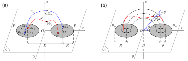
Figure 1.: (a) Sketch of the general magnetic configuration considered in our models constructed with two opposite and magnetic–flux balanced polarities, $P_{+}$ and $P_{-}$. The ${\mathcal{S}}$–surface ($z=0$–plane) symbolizes the photosphere. The two magnetic field lines “a” (blue line) and “c” (red line) show the general connectivity. The magnetic field lines “a” and “c” go from magnetic footpoints $x_{a_{+}}$ and $x_{c_{+}}$ on $S$ to magnetic footpoints $x_{a_{-}}$ and $x_{c_{-}}$ with magnetic fluxes d$\Phi_{a}$ and d$\Phi_{c}$, respectively.. (b) Scheme of the torus configuration. The two polarities ($P_{+}$ and $P_{-}$) are the bases of the torus. The red line represents a magnetic field line of the torus at a radius $\rho$ from its axis. fig:Fig-Methodo-connecti

The considered flux transport velocity field at point $M({\mathbfit x})$ for the two separating polarities model is:

eq:Eq-FTV-sepx$${\mathbfit u}(M) = \mp U_{0}{{\mathbfit e}}_{x}\,,\quad\textrm{for}\ \pm B_{n}(M)>0\,,$$ (11)

where $U_{0}$ is a positive constant. The associated helicity flux density $G_{\theta}$ is therefore (see Appendix app:App-sepx for a detailed derivation):

$$\ilabel{eq:Eq-Gth-sepx}G_{\theta}(M)\ =\ \frac{U_{0}B_{n}(M)}{\pi}\ \frac{{\mathbfit O}_{\mp}{\mathbfit M}\cdot{\mathbfit e}_{y}}{|{\mathbfit O}_{\mp}{\mathbfit M}|^{2}}\ \Phi_{0}\,,\quad\textrm{for}\ \pm B_{n}(M)>0\,,$$ (12)

where $\Phi_{0}$ is the absolute value of the total magnetic flux of each polarity.

For the model of the negative polarity rigidly rotating around the positive one, the flux transport velocity field is:

eq:Eq-FTV-onerot$${\mathbfit u}(M) = {\mathbfit\Omega}\times{{\mathbfit O}}_{+}{\mathbfit M}\,,\quad\textrm{for}\ B_{n}(M)<0\,,$$ (13)

where ${\mathbfit\Omega}=\Omega{\mathbfit e}_{z}$, $\Omega$ being the positive constant rotation rate of the negative polarity. From Appendix app:App-onerot, the associated helicity flux density is non–zero only if $M$ is in the positive polarity, and its expression is given by:

$$\ilabel{eq:Eq-Gth-onerot}G_{\theta}(M)\ =\ -\ \frac{\Omega B_{n}(M)}{2\pi}\ \frac{{\mathbfit O}_{-}{\mathbfit M}\cdot{\mathbfit O}_{+}{\mathbfit O}_{-}}{|{\mathbfit O}_{-}{\mathbfit M}|^{2}}\ \Phi_{0}\,,\quad\textrm{for}\ B_{n}(M)>0\,.$$ (14)

For the third motion model — i.e., two counter–rotating opposite magnetic polarities — the flux transport velocity field is:

eq:Eq-FTV-tworot$${\mathbfit u}(M) = \mp{\mathbfit\Omega}\times{{\mathbfit O}}_{\pm}{\mathbfit M}\,,\quad\textrm{for}\ \pm B_{n}(M)>0\,,$$ (15)

resulting in a helicity flux density (see Appendix app:App-tworot):

$$\ilabel{eq:Eq-Gth-tworot}G_{\theta}(M)\ =\ \mp\frac{\Omega B_{n}(M)}{2\pi}\ \frac{{\mathbfit O}_{\mp}{\mathbfit M}\cdot{\mathbfit O}_{+}{\mathbfit O}_{-}}{|{\mathbfit O}_{\mp}{\mathbfit M}|^{2}}\ \Phi_{0}\,,\quad\textrm{for}\ \pm B_{n}(M)>0\,.$$ (16)

3.2 Magnetic Field

sec:S-Meth-Bfield

Because we want to estimate the precision of the method, it is worthwhile to first consider simple analytical magnetic fields for which the connectivity is theoretically known. This allows us to estimate the precision of our computing method of $G_{\Phi}$.

One simple analytical field to start with is a potential magnetic field (see Figure fig:Fig-Bfieldsa). Such a field is constructed by placing two artificial opposite magnetic charges below the photosphere. The positive and negative magnetic charges are placed at $A_{+}$ and $A_{-}$, resulting in:

$$\ilabel{eq:Eq-Bcharges}{\mathbfit B}({\mathbfit x})=q_{0}\frac{{\mathbfit x}-{\mathbfit x}_{+}}{|{\mathbfit x}-{\mathbfit x}_{+}|^{3}}-q_{0}\frac{{\mathbfit x}-{\mathbfit x}_{-}}{|{\mathbfit x}-{\mathbfit x}_{-}|^{3}}\,,$$ (17)

where ${\mathbfit x}_{\pm}={\mathbfit O}{\mathbfit A}_{\pm}$ and $q_{0}$ is the absolute value of the positive and negative magnetic charges.

Theoretical and numerical simulations studies have shown that, to emerge into the corona, a magnetic flux tube needs some twist Emonet and Moreno-Insertis (1998). Observational studies also highlight that as an AR appears, important amounts of helicity are injected into the corona (e.g., Chae01; Kusano04b; Pariat06; Jeong07; Romano11a; Jing12), with evidences of a twisted flux tube Luoni et al. (2011). Therefore, we consider a second magnetic field defined by a uniformly twisted torus half–emerged into the corona (see panels b and d of Figure fig:Fig-Bfields; Luoni11). The associated magnetic field is ${\mathbfit B}=B_{\theta}{\mathbfit e}_{\theta}+B_{\phi}{\mathbfit e}_{\phi}$, such that:

$$B_{\theta}(M) = \frac{4N\rho}{D+2\rho cos(\theta)}\ B_{\phi}(M)\,,$$

$$B_{\phi}(M) = -B_{0}e^{-\left(\rho/R\right)^{2}}\,,$$ (18)

where $N$ corresponds to the number of turns of the magnetic field lines around the torus axis in half the torus, and $B_{0}$ is the magnetic field strength at the center of the positive polarity. The torus center is located at photospheric point $O$, and the distance $D/2$ defines the main radius of the torus. The variables $\rho$, $\theta$ and $\phi$ are respectively the distance to the torus axis, the rotation angle around the torus axis, and the location angle along the torus axis (see Figure fig:Fig-Methodo-connectib).

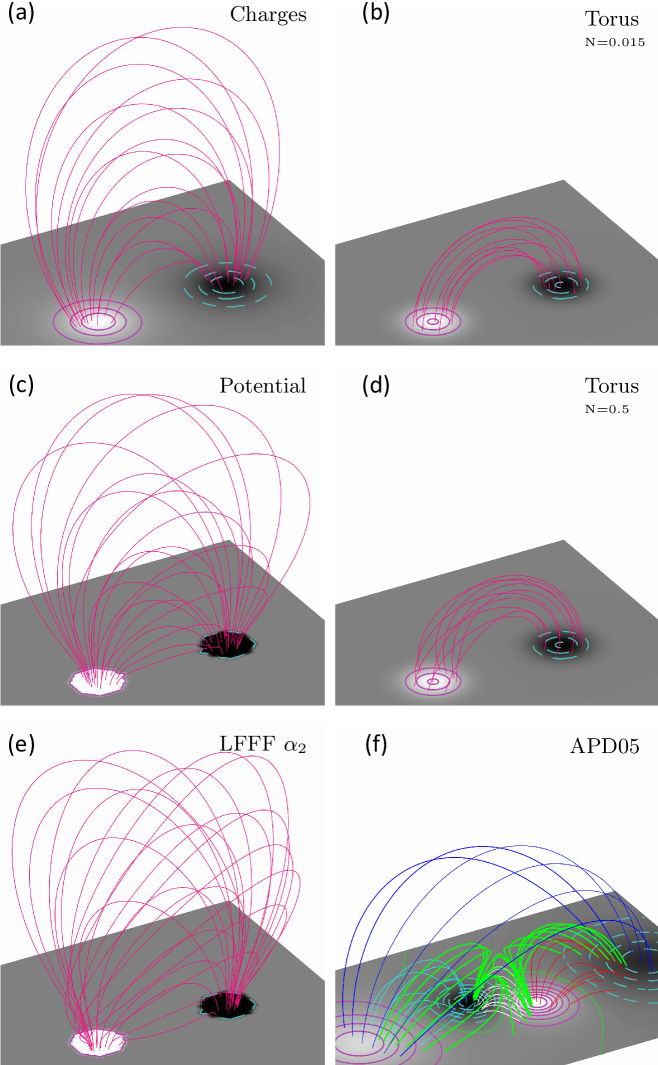
Figure 2.: Magnetic field configurations considered in our investigations. The magnetograms are represented at the $z=0$ plane with superposed isocontours of the magnetic field (cyan dashed and purple solid–lines for negative and positive values of the magnetic field respectively). For all but panel (f), the magnetic field lines are represented by the pink lines and the magnetic field values are between $1000\ \textrm{Gauss}$ (white) and $-1000\ \textrm{Gauss}$ (black). (a) Two magnetic charges. (b,d) Half–emerged torus with a twist $N=0.015$ and $N=0.5$ respectively. (c,e) Two uniform opposite magnetic polarities with linear constant–$\alpha$ force–free field extrapolations $\alpha=0$ and $\alpha=5.6\times 10^{-3}\ \textrm{Mm}^{-1}$ respectively. (f) MHD simulation of a magnetic configuration with quasi–separatrix layers (QSLs). Different colors (red, white, cyan and blue) have been used to show the different quasi–domains of connectivity. Thick green magnetic field lines correspond to QSLs field lines (see Section sec:S-Hinj-in-QSLs). The S–like green line on the magnetogram corresponds to the polarity inversion line. fig:Fig-Bfields

For the two previous cases, the magnetic field is analytical. However, extrapolations of observed magnetograms are in most cases non–analytical fields given on a discrete mesh. The consequence is that errors due to extrapolations and interpolations of the magnetic field will possibly degrade or modify the signal in $G_{\Phi}$ maps. To investigate it, we performed linear force–free field extrapolations (see Figures fig:Fig-Bfieldsc and fig:Fig-Bfieldse) of a magnetogram defined by:

eq:Eq-Buniform$${\mathbfit B}_{z=0}(M) = \pm B_{0}{\mathbfit e}_{z}\,,\quad\textrm{for}\ M\ \textrm{in}\ P_{\pm}\,,$$ (19)

where $B_{0}$ is the magnetic field strength in the positive polarity and, $P_{+}$ and $P_{-}$ refer to the positive and negative magnetic polarities which are circular of radius $R$ (cf Figure fig:Fig-Methodo-connectia). The extrapolations were performed using the code XTRAPOL (e.g., Amari99; Amari06; Amari10). The code solves the Poisson’s equation for the vector potential, ${\bf\nabla}^{2}{\mathbfit A}+\alpha^{2}{\mathbfit A}=0$, with the boundary conditions given by Equation (eq:Eq-Buniform) inside the photospheric polarities and ${\mathbfit B}\cdot{\ \mathrm{d}}{\mathcal{S}}=0$ elsewhere on the boundaries of the extrapolation domain. The vector potential formulation ensures that the solenoidal condition is verified to the machine precision. The boundary conditions assumes that no field go through the lateral and top boundaries. This imposes that the total magnetic flux within the positive polarity is entirely connected to the negative polarity. We make this choice to prevent the presence of open magnetic field lines in the domain in order to compute $G_{\Phi}$ for all photospheric magnetic footpoints of $G_{\theta}$ maps. Note also that, the spatial resolution of the extrapolated fields is chosen to be different from the one used to compute $G_{\theta}$ (see the fragmented shape of the magnetic field isocontours in Figures fig:Fig-Bfieldsc and fig:Fig-Bfieldse). We make this choice to investigate the effect of using a different resolution between the extrapolations and the helicity flux density maps. In practice, we find no significant effects as long as the difference of resolution is lower than $8$ for our high resolution helicity flux density maps. This means that we can use a lower resolution in the extrapolation without modifying the resulting $G_{\Phi}$ map.

The last magnetic configuration considered is more complex as it involves quasi–separatrix layers in MHD simulations. This magnetic field and the associated flux transport velocity fields will be described in Section sec:S-Hinj-in-QSLs.

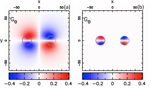
Figure 3.: (a) Full $G_{\theta}$ map of the analytical potential magnetic field (Equation (eq:Eq-Bcharges)). (b) $G_{\theta}$ map for the considered polarities with positive (solid purple) and negative (dashed cyan) isocontours of the magnetic field delimiting these two polarities. fig:Fig-Poltosubpol

For the extrapolated magnetic fields, the magnetic flux is restricted to two circular regions (as defined in Figure fig:Fig-Methodo-connectia). However, this is not strictly the case for the two analytical magnetic fields: even if the field strength strongly decreases away from $O_{\pm}$, it does not vanish. Consequently, there is helicity signal in the whole domain considered in the $G_{\theta}$ and $G_{\Phi}$ maps for the analytical magnetic fields of Equations (eq:Eq-Bcharges) and (eq:Eq-Btorus) as illustrated for $G_{\theta}$ in Figure fig:Fig-Poltosubpola. For coherence of the results, we always extract and consider the helicity flux signal from the two connected polarities of radius R as shown in Figure fig:Fig-Poltosubpolb, and which contain most of the magnetic flux. From now on, the positive and negative polarities $P_{+}$ and $P_{-}$ will refer to these two polarities, and all scalings of Section sec:S-Meth-setup are made with respect to them. However, it must be emphasized that, in all our models, $G_{\Phi}$ computation takes into account the motion of all the magnetic flux at $z=0$.

3.3 Numerical Setup

sec:S-Meth-setup

All maps are computed in a cartesian domain with $400\times 400$ points. The scaling is chosen to take into account the typical values obtained from observations. The $z=0$–plane, which represents the photosphere, covers the $xy$-domain $[-67,67]\times[-67,67]\ \textrm{Mm}^{2}$. The centers of the photospheric polarities are separated by the distance $D=54\ \textrm{Mm}$. The positive and the negative magnetic charges are placed at points $A_{+}$ of coordinates $(-27,0,-13)$ Mm and $A_{-}$ of coordinates $(27,0,-13)$ Mm, respectively. The radius of the photospheric polarities is set to $R=10\ \textrm{Mm}$. The maximum value of the normal component of the magnetic field, $B_{0}$, and of the flux transport velocity fields, $U_{0}$, are set to $1000\ \textrm{Gauss}$ and $0.1\ \textrm{km \ s}^{-1}$ respectively. The extrapolations were performed on a non–uniform mesh covering the domain $[-533,533]\times[-533,533]\times[0,1066]\ \textrm{Mm}^{3}$ with $513\times 513\times 200$ points.

The above scalings lead to helicity flux densities in units of $10^{6}\ \textrm{Wb}^{2}\textrm{.m}^{-2}\textrm{.s}^{-1}$, and a total helicity flux in units of $10^{21}\ \textrm{Wb}^{2}\textrm{.s}^{-1}$ which are typical observed values in ARs (e.g., Chae01; Chandra10).

$G_{\theta}$ maps are computed using Equations (eq:Eq-FTV-sepx) – (eq:Eq-Buniform). Let us first consider the positive magnetic polarity ($B_{n}>0$). In practice, each $G_{\theta}$–mesh point ${\mathbfit x}_{a_{+}}$, is identified as the cross–section of an elementary magnetic flux–tube with the photosphere and is associated to the surface helicity flux density $G_{\theta}({\mathbfit x}_{a_{+}})$ at this point. To compute $G_{\Phi}({\mathbfit x}_{a_{+}})$, we need the position of ${\mathbfit x}_{a_{-}}$ — the second footpoint of the elementary magnetic flux–tube “a” — and its associated surface helicity flux density. Each elementary magnetic flux–tube is thus associated to one magnetic field line that is integrated to get the connectivity. The integration is performed starting from ${\mathbfit x}_{a_{+}}$ to ${\mathbfit x}_{a_{-}}$ using the Fortran NAG–routine D02CJF, with the precision of the integration defined as $10^{-n}$. Thus, the higher $n$ is, the more precisely the connectivity and $G_{\Phi}$ are computed. Generally, the ${\mathbfit x}_{a_{-}}$ footpoint does not fall on a mesh point. Thus, the values of $G_{\theta}$ and $B_{n}$ at this point are bilinearly interpolated using the values at the four closest surrounding mesh points. If ${\mathbfit x}_{a_{-}}$ is not found on the ($z=0$)–plane (e.g., open magnetic field lines), the value of $G_{\Phi}$ at ${\mathbfit x}_{a_{+}}$ is simply set to $G_{\theta}({\mathbfit x}_{a_{+}})$. Finally, the same procedure as above is used in the negative magnetic polarity ($B_{n}<0$) starting the magnetic field line integration from ${\mathbfit x}_{a_{-}}$.

4 Results for Two Magnetic Charges

sec:S-two-source-charges

In this section, the magnetic field is given by Equation (eq:Eq-Bcharges) for all flux transport velocity models and the associated magnetogram at the $z=0$–plane is displayed in Figure fig:Fig-Bfieldsa.

4.1 Two Separating Magnetic Polarities

sec:S-Charges-sepx

In this example, the two connected opposite magnetic polarities separate away from each other in the $x$-direction (see Equation (eq:Eq-FTV-sepx)). Since the polarities simply separate without any rotation, no helicity is injected to the system. However, as the two polarities separate, every elementary polarity sees a relative rotation of all other elementary polarities of opposite sign. This induces net non–zero values of $G_{\theta}$ as shown in the left panel of Figure fig:Fig-Charges-sepxa.

In this model, the symmetry of the magnetic field and of the applied velocity field implies $G_{\theta}({\mathbfit x}_{a_{-}})=-G_{\theta}({\mathbfit x}_{a{+}})$. Therefore, by taking the connectivity into account, $G_{\Phi}$ is null to the numerical errors over all the two polarities (Figure fig:Fig-Charges-sepxb). This simple example reveals the limits of $G_{\theta}$ to present a truthful distribution of helicity flux while $G_{\Phi}$ gives the expected results.

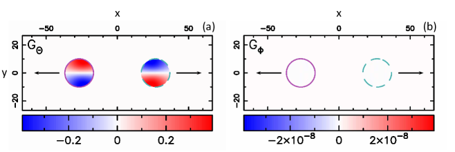
Figure 4.: Helicity flux density distribution, in $10^{6}\ \textrm{Wb}^{2}\textrm{m}^{-2}\textrm{s}^{-1}$, for the case of two separating opposite magnetic polarities without rotation. (a) $G_{\theta}$ map. (b) $G_{\Phi}$ map. Solid purple and dashed cyan are isocontours of the magnetic field. Black arrows show the motion applied to the polarities. The saturation levels of $G_{\theta}$ and $G_{\Phi}$ are different by eight orders of magnitude. fig:Fig-Charges-sepx

4.2 One Polarity Rigidly Rotating Around the Other

sec:S-Charges-onerot

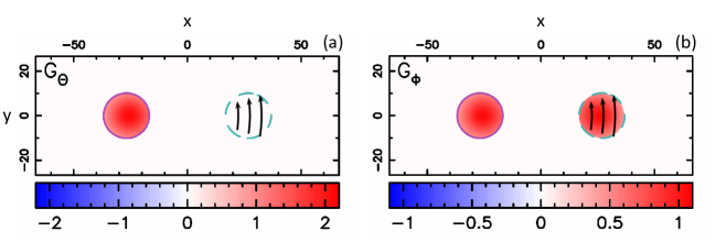
Figure 5.: Helicity flux density distribution, in $10^{6}\ \textrm{Wb}^{2}\textrm{m}^{-2}\textrm{s}^{-1}$ for the negative polarity rigidly rotating around the positive polarity. The drawing convention is the same as in Figure fig:Fig-Charges-sepx (with a different color scale). fig:Fig-Charges-onerot

The positive polarity is fixed while the negative polarity rigidly rotates around $O_{+}$ (the center of the positive polarity, see Equation (eq:Eq-FTV-onerot)). From Equation (eq:Eq-Gth-onerot), $G_{\theta}$ is non–zero only in the positive polarity. The reason is that, in Equation (eq:Eq-Gtheta), there are two terms that contribute to $G_{\theta}$ inside one polarity. One term is the relative motion of footpoints inside the polarity. The second is the relative motion with regard to the footpoints of the other polarity. In the negative polarity, the two terms cancel out (Appendix app:App-onerot). In the positive polarity, however, only the term coming from the relative motion of the negative polarity is non–zero.

This second example also presents the limits of $G_{\theta}$ maps to well localize the injection of helicity. This can be misleading when relating the injection of helicity to magnetic activity (e.g., Chandra10). This is corrected in the corresponding $G_{\Phi}$ map that shows that positive helicity is redistributed in both polarities (Figure fig:Fig-Charges-onerotb).

4.3 Two Counter–rotating Polarities

sec:S-Charges-tworot

Let us now consider the model of two counter–rotating polarities (Equation (eq:Eq-FTV-tworot)). The positive and negative polarities rigidly rotate clockwisely and counterclockwisely around their centers $O_{+}$ and $O_{-}$, respectively. This configuration illustrates the difference of assumptions in the definition of $G_{\theta}$ and $G_{\Phi}$.

Indeed, if the rotation is slow enough, the system is equivalent to a non-twisted flux tube rotating around its central axis. With such driving, a non-twisted flux tube would appear similarly untwisted at any time. Thus, overall no helicity is injected to the system. One therefore expects that $G_{\Phi}$ would correspond to this null injection of magnetic helicity.

The $G_{\theta}$ map presents a distribution of helicity which is far different from a null injection (Figure fig:Fig-Charges-tworota). Taking the connectivity into account, i.e., using $G_{\Phi}$ (Figure fig:Fig-Charges-tworotb), removes this helicity flux signal (regardless of numerical errors) allowing to get the expected null distribution of helicity flux.

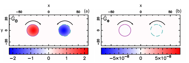
Figure 6.: Helicity flux density distribution, in $10^{6}\ \textrm{Wb}^{2}\textrm{m}^{-2}\textrm{s}^{-1}$ for the two counter–rotating opposite magnetic polarities. The drawing convention is the same as in Figure fig:Fig-Charges-sepx (with a different color scale). fig:Fig-Charges-tworot

While $G_{\theta}$ clearly misrepresents the global slow injection of helicity in this case, it would properly represent the helicity injection if the considered motion was extremely fast. Indeed if one considers counter rotating motions at a speed higher than the Alfvénic transit time, the opposite footpoint would have no indication of the helicity injection at the other footpoint. At the beginning of the injection, an initially untwisted flux rope would be such that the central part would stay untwisted but with oppositely twisted field around each footpoint. These counter–rotating motions would correspond to the launch of two rotating Alfvén waves of opposite sign. The $G_{\theta}$ maps do properly represent such helicity injection. As time goes, these Alfvén waves would eventually cancel each other resulting in a null helicity budget for the system. For longer timescales, the $G_{\Phi}$ map therefore better represents the proper helicity injection in the system.

4.4 Errors Estimation

sec:S-Charges-error

In this section, we investigate the role of the parameter n — used for field lines integration — in the above $G_{\Phi}$ maps. $G_{\theta}$ and the connectivity are analytically known which allows us to compute the theoretical value, $G_{\Phi,\rm{th}}$. Then, we estimate the error between the computed $G_{\Phi}$ map from our numerical method and $G_{\Phi,\rm{th}}$ by computing the root mean square of $G_{\Phi}-G_{\Phi,\rm{th}}$.

With the analytical magnetic field considered in this section, the resolution on the magnetic field is only limited by the computing precision, i.e., $10^{-16}$ as the magnetic field was computed with a double precision. The numerical precision on $G_{\Phi}$ is thus limited by the precision of:

$\cdot$ $G_{\theta}$, ${\rm{err}}_{G_{\theta}}\approx 10^{-16}$,

$\cdot$ the field lines integration, ${\rm{err}}_{{\rm{fli}}}\approx 10^{-n}$,

$\cdot$ the computation of $B_{n}$ at the second footpoint, ${\rm{err}}_{B_{n}}\approx 10^{-16}$,

$\cdot$ the bilinear interpolation of $G_{\theta}$ at the second footpoint, ${\rm{err}}_{{\rm{interp}}}$.

The total error at each mesh point, ${\rm{err}}_{{\rm{tot}}}$, can thus be estimated as follows:

$$\ilabel{eq:Eq-guesstimated-error}{\rm{err}}_{{\rm{tot}}}\approx\sqrt{{\rm{err}}_{G_{\theta}}^{2}+{\rm{err}}_{{\rm{fli}}}^{2}+{\rm{err}}_{B_{n}}^{2}+{\rm{err}}_{{\rm{interp}}}^{2}}\,.$$ (20)

For smooth variations of $G_{\theta}$ (as in all our cases), the error from the bilinear interpolation should not be the most limiting one. In this case, for $n<16$, the precision on $G_{\Phi}$ is expected to be limited by the precision of field line integration. The consequence is that we expect an exponential decrease of the error as $n$ increases.

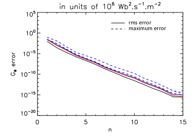
Figure 7.: Computed root mean square (solid lines) and maximum error (dashed lines) from $G_{\Phi}$ maps for two separating polarities (black), the negative polarity rigidly rotating around the positive one (red), and two counter–rotating magnetic polarities (blue), as a function of the field line integration parameter $n$ defining the numerical integration precision ($=10^{-n}$). fig:Fig-Charges-error

Figure fig:Fig-Charges-error displays the influence of n on the root mean square and the maximum error of $G_{\Phi}$ maps. As expected, the figure shows that both $G_{\Phi}$ rms and maximum error exponentially decrease as $n$ increases. Therefore, the precision on $G_{\Phi}$ is indeed limited by the precision of field lines integration. The rms on $G_{\Phi}$, for the three cases shown Figures fig:Fig-Charges-sepx – fig:Fig-Charges-tworot ($n=8$), is $2$, $5$ and $7\times 10^{-10}$ $G_{\theta}$ units respectively, i.e., more than $10^{9}$ times smaller than the typical values of the signal found in $G_{\theta}$ maps. Hence, our numerical method allows us to compute the distribution of helicity flux, $G_{\Phi}$, with a very good accuracy.

5 Results for a Half Emerged Torus

sec:S-Torus

In this section, the magnetic field is a uniformly twisted torus half emerged into the solar corona (see Figures fig:Fig-Bfieldsb and fig:Fig-Bfieldsd and Equation (eq:Eq-Btorus); Luoni11). The two opposite magnetic polarities are thus the two intersections of the torus with the photosphere (Figure fig:Fig-Methodo-connectib).

The amount of helicity, $H$, found in ARs can be converted to a uniform twist, $N^{\prime}$, with $H=N^{\prime}\Phi^{2}$, where $\Phi$ is the AR magnetic flux (average of both polarities). Observations report typical values of $N^{\prime}$ from $\approx 0.01$ to $\approx 0.3$ (Demoulin09 and references therein). In the following, we thus consider the torus configuration with $N=0.015$, $0.05$, and $0.5$.

Note that, the case $N=0$ has the same type of connectivity as the two magnetic charges but with a different $B_{n}$ distribution. Therefore, we expect similar helicity flux distributions as in Figures fig:Fig-Charges-sepx – fig:Fig-Charges-tworot when the same velocity models are applied.

5.1 Two Separating Magnetic Polarities

sec:S-Torus-sepx

As for the potential magnetic field of Section sec:S-Charges-sepx, the two polarities separate without any rotation (flow given by Equation (eq:Eq-FTV-sepx)) implying that no helicity is injected to the system. As expected, $G_{\theta}$ (Figure fig:Fig-Torus-sepxa) exhibits a similar distribution as for the case with two magnetic charges (Figure fig:Fig-Charges-sepxa), and the total helicity flux computed from $G_{\theta}$ and $G_{\Phi}$ maps is indeed zero (Section sec:S-Charges-sepx). However, as shown by Figure fig:Fig-Torus-sepxb-d, $G_{\Phi}$ maps also present helicity injection with both signs of helicity in both polarities. But are these signals in $G_{\Phi}$ maps real, or are they spurious signals as in the $G_{\theta}$ map?

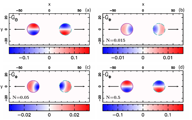
Figure 8.: $G_{\theta}$ and $G_{\Phi}$ maps for the torus magnetic field configuration with two separating magnetic polarities. (a) $G_{\theta}$ map. (b,c,d) $G_{\Phi}$ maps for a twist $N=0.015$, $0.05$ and $0.5$ respectively. The drawing convention is the same as in Figure fig:Fig-Charges-sepx (notice the different color scales). fig:Fig-Torus-sepx

Demoulin06, show that the total magnetic helicity flux in ${\mathcal{V}}$ can be written as the summation of the mutual helicity of all pairs of elementary magnetic flux tubes contained in ${\mathcal{V}}$, i.e., the total magnetic helicity of the system can be rewritten as:

$$\ilabel{eq:Eq-MutualH}H=\frac{1}{2\pi}\int_{\Phi_{\pm}}\int_{\Phi_{\pm}}{\mathcal{L}}_{a,c}{\ \mathrm{d}}\Phi_{a_{+}}{\ \mathrm{d}}\Phi_{c_{+}}\,,$$ (21)

with ${\mathcal{L}}_{a,c}$, the mutual helicity between the two magnetic flux tubes “a” and “c”. Comparing the time derivative of Equation (eq:Eq-MutualH):

$$\ilabel{eq:Eq-HFlux-vs-MutualH}\frac{{\mathrm{d}}H}{{\mathrm{d}}t}=\frac{1}{2\pi}\int_{\Phi_{\pm}}\int_{\Phi_{\pm}}\frac{{\mathrm{d}}{\mathcal{L}}_{a,c}}{{\mathrm{d}}t}{\ \mathrm{d}}\Phi_{a_{+}}{\ \mathrm{d}}\Phi_{c_{+}}\,,$$ (22)

to Equations (eq:Eq-dH-Phi-doubleInt) and (eq:Eq-dhdens-Phi) implies:

$$\frac{{\mathrm{d}}{\mathcal{L}}_{a,c}}{{\mathrm{d}}t}\; = \;\frac{{\mathrm{d}}\theta({\mathbfit x}_{c_{+}}-{\mathbfit x}_{a_{-}})}{{\mathrm{d}}t}+\frac{{\mathrm{d}}\theta({\mathbfit x}_{c_{-}}-{\mathbfit x}_{a_{+}})}{{\mathrm{d}}t}$$ (23)

$$\!\!\!-\frac{{\mathrm{d}}\theta({\mathbfit x}_{c_{+}}-{\mathbfit x}_{a_{+}})}{{\mathrm{d}}t}-\frac{{\mathrm{d}}\theta({\mathbfit x}_{c_{-}}-{\mathbfit x}_{a_{-}})}{{\mathrm{d}}t}\,.$$

By integrating Equation (eq:Eq-MutualH-Flux) in time, they express the mutual helicity of two magnetic field lines “a” and “c” as a function of the angles between their photospheric footpoints. Using the convention that field line “c” is above field line “a”, they obtain:

$$\ilabel{eq:Eq-MutualH-angles}{\mathcal{L}}_{a,c}={\mathcal{L}}^{\rm arch}_{a,\hat{\mathbf{c}}}=\frac{1}{2\pi}\left(\alpha_{c_{+}}+\alpha_{c_{-}}\right)\,,$$ (24)

where $\alpha_{c_{\pm}}$ is the angle between segments $c_{\pm}a_{\pm}$ and $c_{\pm}a_{\mp}$ and is defined in the interval $[-\pi,\pi]$ with the trigonometric convention (Figure fig:Fig-Torus-mutualHa). The consequence is that any change in these angles will lead to a variation of mutual helicity and thus, a flux of magnetic helicity (Equations (eq:Eq-HFlux-vs-MutualH) – (eq:Eq-MutualH-angles)).

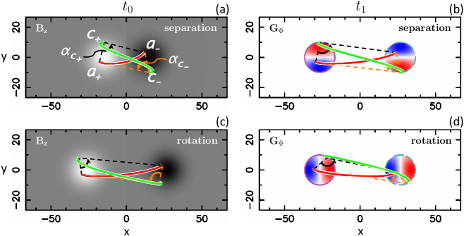
Figure 9.: Torus configuration for the twist $N=0.5$ illustrating the change in mutual magnetic helicity between two magnetic field lines (red and green lines) at two different times ($t_{1}>t_{0}$) and at $z=0$. (a,b) Two separating magnetic polarities (as in Figure fig:Fig-Torus-sepx). (c,d) Counter–rotating polarities (as in Figure fig:Fig-Torus-tworot). Left column: Normal component of the magnetic field at $t_{0}$. The values of the magnetic field are in the range $-1000\ \textrm{G}$ (black) to $1000\ \textrm{G}$ (white). Right column: Distribution of $G_{\Phi}$ at $t_{1}$. The angle between segments $c_{\pm}a_{\pm}$ and $c_{\pm}a_{\mp}$ represents the angle $\alpha_{c_{\pm}}$ of Equation (eq:Eq-MutualH-angles). The change in the relative orientation of the red and green magnetic field lines that leads to the change in $\alpha_{c_{\pm}}$ — right panel compared with left panel — is a clear evidence of mutual magnetic helicity changes of the two field lines between $t_{0}$ and $t_{1}$. fig:Fig-Torus-mutualH

Let us consider the two magnetic field lines “a” and “c” starting at $a_{+}$ and $c_{+}$ and ending at $a_{-}$ and $c_{-}$, respectively represented by the red and green lines in Figure fig:Fig-Torus-mutualH of the torus for $N=0.5$. As the two polarities of the torus separate away from each other in the $x$-direction, the $y$-coordinate of all four footpoints remains unchanged. Hence, the orientation of the segments $c_{\pm}a_{\pm}$ remains also the same, and only segments $c_{\pm}a_{\mp}$ change of orientation. In particular, the geometry implies that $\alpha_{c_{\pm}}$ increases as the polarities separate in the case shown in Figure fig:Fig-Torus-mutualH for $N=0.5$. Therefore, the separation induces a positive variation of mutual helicity of “a” and “c”.

More generally, there is always an increase of mutual helicity of the magnetic field line “c” in Figures fig:Fig-Torus-mutualHa and fig:Fig-Torus-mutualHb with any other magnetic field line “a” inside the polarities: as the polarities separate, there is always an increase of $\alpha_{c_{\pm}}$ for any “a” within the polarities. This results in a net positive change of mutual helicity for “c” with regard to all the other “a”, and thus, a net positive helicity flux $G_{\Phi}$ at the footpoint location of “c”.

A more precise geometrical analysis — i.e., using the general definition of ${\mathcal{L}}_{a,c}$ in Equation (32) of Demoulin06 — reveals that, for the magnetic field lines footpoints of the $y>0$ (resp. $y<0$) part of the positive polarity, there is a net positive (resp. negative) variation of mutual helicity with a magnitude decreasing with $y$ (resp. increasing with $-y$).

For $N$ close to $0\ [1]$ (i.e., modulo $1$) turn, there is a similar behavior, except that the origin $O=(0,0)$ is no longer a center of symmetry for the magnetic footpoints. In particular, at these values of N, we find that, for the most externe (resp. interne) magnetic field lines, there is a net positive (resp. negative) variation of mutual helicity leading to a net positive (resp. negative) helicity flux (Figure fig:Fig-Torus-sepx). However, the helicity flux at these $N$ values is typically ten times smaller when $N=0.015\ [1]$ than for the $N=0.5\ [1]$ case. As $N$ gets closer to $0.5\ [1]$ turn, the magnetic field lines are more twisted and they share more mutual helicity, i.e., the angles between the footpoints of two field lines are larger. The consequence is that, the change in the angles between footpoints, i.e., in their mutual helicity, will be higher as the two polarities separate, tending towards the helicity flux distribution of Figure fig:Fig-Torus-sepx as $N$ gets closer to $0.5\ [1]$ turn.

Therefore, the signal in the $G_{\Phi}$ maps of Figure fig:Fig-Torus-sepx is due to a variation of mutual helicity between magnetic field lines as the two polarities separate, and thus, is a real signal.

5.2 One Polarity Rigidly Rotating Around the Other

sec:S-Torus-onerot

The flux transport velocity field is given by Equation (eq:Eq-FTV-onerot). As in Section sec:S-Charges-onerot, the helicity flux density distribution computed using $G_{\theta}$ only presents helicity flux in the positive polarity as in Figure fig:Fig-Charges-onerota. The computation of helicity injection using $G_{\Phi}$ removes this problem and the associated flux is typically twice smaller than in $G_{\theta}$, but present on both polarities independently of N value (comparable to Figure fig:Fig-Charges-onerotb).

5.3 Two Counter–rotating Polarities

sec:S-Torus-tworot

As pointed out in Section sec:S-Charges-tworot, for slow enough motions of the flux transport velocity field (given by Equation (eq:Eq-FTV-tworot)), this model is equivalent to a cylinder rotating around its axis. The only difference is that, now, the cylinder has twisted magnetic field lines. The presence of twisted field lines, though, does not change the fact that no helicity is globally injected to the system.

The instantaneous footpoint injections displayed by the $G_{\theta}$ map, Figure fig:Fig-Torus-tworota, are similar to those in Figure fig:Fig-Charges-tworota. They would be meaningful for very fast motions.

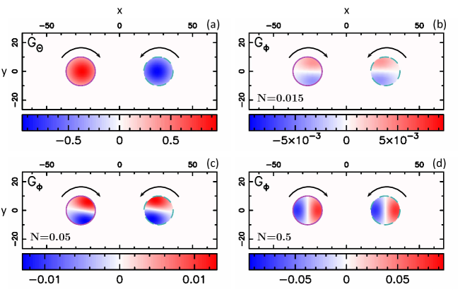
Figure 10.: $G_{\theta}$ and $G_{\Phi}$ maps for the torus magnetic field configuration with two counter–rotating magnetic polarities. (a) $G_{\theta}$ map. (b,c,d) $G_{\Phi}$ maps for $N=0.015$, $0.05$ and $0.5$ respectively. The drawing convention is the same as in Figure fig:Fig-Charges-sepx (notice the different color scales). fig:Fig-Torus-tworot

Considering $G_{\Phi}$ maps, the distribution changes significantly depending on the degree of twist (Figure fig:Fig-Torus-tworot). While the global injection stays null, $G_{\Phi}$ maps reveal subtle effects of mutual helicity variation between the twisted lines within the flux rope. Because of the twist, the magnetic field lines of the torus share mutual helicity between each other as the flux rope globally rotates around its axis. In a way similar to what has been discussed in Section sec:S-Torus-sepx, as the two polarities counter–rotate, the relative orientation of the magnetic field lines within the flux rope changes: cf. Figures fig:Fig-Torus-mutualHc and fig:Fig-Torus-mutualHd. The magnitude of this variation increases with the number of turns, $N$, of the magnetic field lines around the torus axis. This induces a net change of mutual helicity between the magnetic field lines revealed by the $G_{\Phi}$ maps of Figure fig:Fig-Torus-tworot. This process is completely hidden by the $G_{\theta}$ maps which are completely independent of the twist amount.

The use of $G_{\Phi}$ is here crucial to understand the variation of mutual magnetic helicity driven by photospheric footpoint motions.

6 Results for Extrapolated Magnetic Fields

sec:S-Uniform

In observational studies, extrapolations of the magnetic field will be used to infer the connectivity. Hence, in our tests, we consider extrapolated magnetic fields in order to study the influence of using them on the precision of the connectivity and thus, of $G_{\Phi}$.

In this section, we consider two uniform opposite magnetic polarities with $B_{0}=1000\ G$ in the positive polarity and $-1000\ G$ in the negative polarity. Three linear force–free fields are considered in all our three flux transport velocity fields investigated: a potential field, and two linear force–free fields with a force–free parameter equal to $\alpha_{1}=10^{-3}$ and $\alpha_{2}=5.6\times 10^{-3}\ \textrm{Mm}^{-1}$ (Figures fig:Fig-Bfieldsc and fig:Fig-Bfieldse) which are typical values derived from observations (see e.g., Pevtsov95; Longcope03; Green02b; Chandra10).

6.1 Two Separating Magnetic Polarities

sec:S-Uniform-sepx

In this section, we study the distribution of helicity flux density for the two separating magnetic polarities case (see Equation (eq:Eq-FTV-sepx)).

First, let us consider the potential field ($\alpha=0$, Figure fig:Fig-Uniform-sepxb). With this magnetic field configuration, the model is analogous to the one considered Section sec:S-two-source-charges. Consequently, as in Section sec:S-Charges-sepx, we expect no signal in the $G_{\Phi}$ map as no helicity is injected to the system. This is well shown in Figure fig:Fig-Uniform-sepxb where the helicity flux signal is indeed null to the numerical errors.

Let us now consider the two linear force–free magnetic field configurations. These configurations are analogous to the torus one (for $N\neq 0$) in the sense that magnetic field lines now have non–null mutual helicity. Therefore, as the two polarities separate away from each other, the angles between magnetic field lines footpoints change. This results in a variation of mutual helicity between field lines inducing a local flux of magnetic helicity as shown in Figures fig:Fig-Uniform-sepxc and fig:Fig-Uniform-sepxd. However, the total helicity flux is indeed zero as expected (Section sec:S-Torus-sepx).

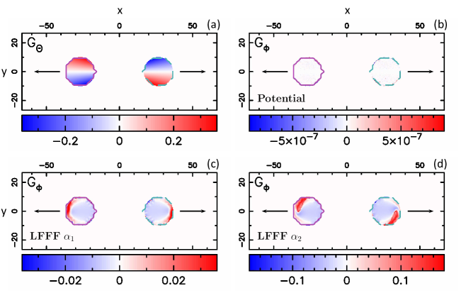
Figure 11.: $G_{\theta}$ and $G_{\Phi}$ maps for the extrapolated magnetic field configurations with two separating magnetic polarities. (a) $G_{\theta}$ map. (b,c,d) $G_{\Phi}$ maps for the linear force–free fields $\alpha=0$ (potential), $\alpha_{1}=10^{-3}$ and $\alpha_{2}=5.6\times 10^{-3}\ \textrm{Mm}^{-1}$. The drawing convention is the same as in Figure fig:Fig-Charges-sepx (notice the different color scales). fig:Fig-Uniform-sepx

Note also that, while the $G_{\theta}$ map exhibits, in each polarity, two regions of strong net opposite helicity flux (symmetric with regard to the $x$-axis), the $G_{\Phi}$ maps present a diffuse (concentrated) region of negative (positive) flux in the inner (most external) part of the system, respectively. In addition, the higher the linear force-free field constant–$\alpha$ is (in magnitude), the higher is the magnitude of the helicity flux signal in each polarity. These results are in agreement with the ones for the torus case and, again, demonstrate the limits of the $G_{\theta}$ proxy.

6.2 One Polarity Rigidly Rotating Around the Other

sec:S-Uniform-onerot

In this section, the negative polarity rigidly rotates around the center of the positive polarity (Equation (eq:Eq-FTV-onerot)).

Because $G_{\theta}$ does not take the magnetic field lines connectivity into account, it is not able to show that helicity is injected in both magnetic polarities. As in Sections sec:S-Charges-onerot and sec:S-Torus-onerot, $G_{\Phi}$ proxy displays the true distribution of helicity flux, which is positive in both positive and negative polarities and twice smaller than with $G_{\theta}$ in the positive polarity (comparable to Figure fig:Fig-Charges-onerot).

6.3 Two Counter–rotating Polarities

sec:S-Uniform-tworot

The two opposite magnetic polarities are counter–rotating around their own center (Equation (eq:Eq-FTV-tworot)). We recall that this model is equivalent to the rotation of a cylinder around its axis, and hence, no helicity is globally injected to the system.

For the same reasons as in Section sec:S-Charges-tworot, the $G_{\Phi}$ map of the potential magnetic field case has zero values (to the numerical errors) everywhere. As indicated by Figure fig:Fig-Uniform-tworot, the $G_{\Phi}$ maps for the two linear force–free fields ($\alpha\neq 0$) present non–zero helicity fluxes with both signs in both polarities. As for the torus case ($N\neq 0$), the signal in $G_{\Phi}$ maps is real as there is a change of mutual helicity between magnetic field lines as the two polarities rotate.

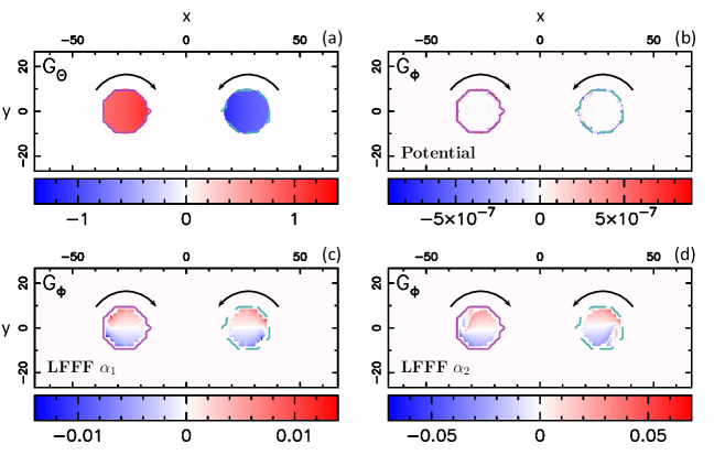
Figure 12.: $G_{\theta}$ and $G_{\Phi}$ maps for the extrapolated magnetic field configurations with two counter–rotating magnetic polarities. (a) $G_{\theta}$ map. (b,c,d) $G_{\Phi}$ maps for the linear force–free fields $\alpha=0$ (potential), $\alpha_{1}=10^{-3}$ and $\alpha_{2}=5.6\times 10^{-3}\ \textrm{Mm}^{-1}$. The drawing convention is the same as in Figure fig:Fig-Charges-sepx (notice the different color scales). fig:Fig-Uniform-tworot

6.4 Errors Estimation

sec:S-Uniform-error

As in Section sec:S-Charges-error, we estimate the computation errors due to the magnetic field lines integration as a function of the field lines integration parameter $n$. An analytical connectivity is available for the potential field since it has the same type of connectivity as the two magnetic charges (although with a different $B_{n}$ distribution). Then, it is straightforward to compute the theoretical $G_{\Phi,\rm{th}}$ value for each flux transport velocity model and the errors.

As expected, Figure fig:Fig-Uniform-error shows that both $G_{\Phi}$ rms and maximum error exponentially decrease as $n$ increases. However, it also shows a saturation of the errors to $10^{-6}-10^{-4}$ $G_{\theta}$ units for $n>6$. In particular, the rms on $G_{\Phi}$ (black, red and blue solid lines) saturate at $0.2$, $7$ and $8\times 10^{-5}$ $G_{\theta}$ units respectively.

The use of an extrapolated magnetic field implies that the magnetic field is discretized. Hence, at each step of the integration of magnetic field lines, the magnetic field is interpolated and not analytically computed. This affects the precision on the computation of $B_{n}$ and $G_{\theta}$ at the second footpoint of each magnetic field line, i.e., enhances the terms ${\rm{err}}_{B_{n}}$ and ${\rm{err}}_{{\rm{interp}}}$ in Equation (eq:Eq-guesstimated-error). This is well illustrated in Figure fig:Fig-Uniform-error where the choice of $n$ dominates the precision of $G_{\Phi}$ only up to $n=6$. Even though the precision reached on $G_{\Phi}$ is much less for $n>6$ than in the potential analytical case (Section sec:S-two-source-charges), our method still allows us to compute the true distribution of helicity injection with a good accuracy.

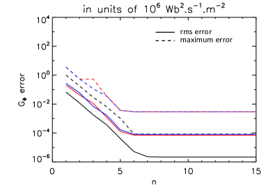
Figure 13.: Computed root mean square (solid lines) and maximum error (dashed lines) from $G_{\Phi}$ maps as a function of the field line integration parameter $n$ defining the numerical integration precision ($=10^{-n}$). This plot is similar to Figure fig:Fig-Charges-error but done for an extrapolated potential field. Three boundary flows are shown: two separating polarities (black), the negative polarity rigidly rotating around the positive one (red), and two counter–rotating magnetic polarities (blue). fig:Fig-Uniform-error

7 Results for Magnetic Fields Containing Quasi-separatrix Layers

sec:S-Hinj-in-QSLs

In this section, we investigate the helicity injection at the $z=0$–plane in two quadrupolar magnetic field configurations with quasi-separatrix layers (QSLs), from the simulations of Aulanier05. Our goal is to study the quality of our method when strong connectivity gradients are present.

7.1 QSLs

sec:S-QSLs

QSLs are regions where the magnetic field lines connectivity changes continuously with very sharp gradients with the limit case of separatrices when gradients are infinite Démoulin, Priest, and Lonie (1996); Titov, Hornig, and Démoulin (2002). Even in the cases with continuous connectivity changes, QSLs are preferential sites for current layers formation (see Aulanier05 and references therein).

The concept of QSLs has been intensively studied and developed in the last two decades (see review by Demoulin06Review and references therein) and observational data analyses have reported the presence of such topological structures in the solar atmosphere (e.g., Demoulin97; Mandrini97, 2006; Bagala00; Masson09; Baker09; Savcheva12). QSLs are defined as regions where the squashing degree, $Q$, is much larger than $2$ Titov, Hornig, and Démoulin (2002). If we consider an elementary flux tube — within a QSL — with one circular photospheric footpoint, then $Q$ is a measure of the squashing of the section of this elementary flux tube at the other photospheric footpoint. Configurations with QSLs are thus cases for which a connectivity–based helicity flux density is required to localize the true site(s) of helicity injection and, e.g., , study its role in the trigger of eruptive events.

7.2 Initial Magnetic Field Configurations and Flux Transport Velocities

sec:S-QSLs-Initial

In the following, we consider the magnetic field configurations from the simulations of Aulanier05 on the formation of current layers in QSLs (Figure fig:Fig-Bfieldsf). The magnetic configurations are referred to as $\Phi=120^{\circ}$ and $\Phi=150^{\circ}$ where $\Phi$ describes the angle between the inner and outer dipoles. For each magnetic configuration, two flux transport velocity fields are considered: a nearly solid translation in the $y$-direction and a nearly solid rotation of the positive polarity of the inner dipole (see Sections 2,3 and Figure 5 of Aulanier05 for further detailed informations on the setup). For simplicity, the positive and negative polarities of the inner or outer dipole will be referred to as IP and IN, or OP and ON, respectively.

7.3 Results with Twisting Motions

sec:S-QSLs-twist

In this model, the IP polarity nearly rigidly rotates counterclockwisely around its center. The flux transport velocity field is given by Equations (13) and (14) of Aulanier05. In terms of helicity flux density, we can analytically show that $G_{\theta}({\mathbfit x})=0$ when ${\mathbfit x}$ is not in IP and $G_{\theta}({\mathbfit x}\ \textrm{in}\ \rm{IP})<0$. For $G_{\Phi}$ on the other hand, because the twisting motion is applied to one part of the QSLs, we expect to see two regions of a twice smaller helicity flux: in IP and in the part of the QSLs connected to it.

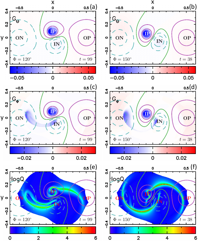
Figure 14.: Results of two MHD simulations with a nearly solid rotation of the inner magnetic polarity (IP) and no motion in other polarities. The angle between the inner and outer bipoles is $\Phi=120^{\circ}$ (left column) and $\Phi=150^{\circ}$ (right column) and the simulation time is $t=99$ and $t=38$ Alfvén times respectively. The panels show the photospheric distribution of: (a,b) $G_{\theta}$, (c,d) $G_{\Phi}$, and (e,f) ${\rm{log}}_{10}Q$. The green line corresponds to the polarity inversion line, while the solid purple (resp. dashed cyan) are positive (resp. negative) isocontours of the magnetic field. fig:Fig-QSLs-twist

Figure fig:Fig-QSLs-twist displays the results of the $G_{\theta}$ (top row) and $G_{\Phi}$ (middle row) computations for the $\Phi=120^{\circ}$ (left column) and $150^{\circ}$ (right column) configurations. As expected, $G_{\theta}$ maps present a negative helicity flux distributed only in IP.

In the $G_{\Phi}$ maps, two main distinct regions of negative helicity flux are present (Figures fig:Fig-QSLs-twistc and fig:Fig-QSLs-twistd). The first region, IP, has a flux twice smaller than in $G_{\theta}$ as expected (notice the factor $1/2$ between $G_{\theta}$ and $G_{\Phi}$ color scales). The second region corresponds to the QSL portion connected to IP. The helicity flux is more concentrated on the edges of the QSL in both ON and IN (see $G_{\Phi}$ compared to ${\rm{log}}_{10}Q$ maps). This effect is even more important for the $\Phi=150^{\circ}$ configuration (Figure fig:Fig-QSLs-twistd). This is due to the $|B_{n}({\mathbfit x}_{a_{-}})/B_{n}({\mathbfit x}_{a_{+}})|$ ratio which is much smaller than unity in between ON and IN. Hence, from Equation (eq:Eq-Gphi), it results that the helicity flux density is much weaker in the center of the QSL than at its edges. Because in the $\Phi=120^{\circ}$ configuration, IN and ON are closer to each other, the region of weak $B_{n}$ is smaller and the helicity flux distribution appears less concentrated at the edges of the QSL than for the $\Phi=150^{\circ}$ configuration (Figures fig:Fig-QSLs-twistc and fig:Fig-QSLs-twistd).

Finally, we notice that, the positive helicity flux signal in $G_{\Phi}$ maps (Figures fig:Fig-QSLs-twistc and fig:Fig-QSLs-twistd) is a remnant spurious signal already present in $G_{\theta}$ maps, as the velocity field is not numerically limited to IP.

7.4 Results with Translational Motions

sec:S-QSLs-trans

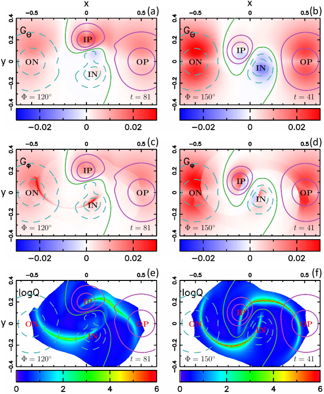
Figure 15.: Results of two MHD simulations with a nearly solid translation of the inner magnetic polarity (IP) and nearly no motion in other polarities. The angle between the inner and outer bipoles at $t=0$ is $\Phi=120^{\circ}$ (left column) and $\Phi=150^{\circ}$ (right column) and the simulation time is $t=81$ and $t=41$ Alfvén times respectively. The panels show the photospheric distribution of: (a,b) $G_{\theta}$, (c,d) $G_{\Phi}$, and (e,f) ${\rm{log}}_{10}Q$. The drawing convention is the same as in Figure fig:Fig-QSLs-twist. fig:Fig-QSLs-trans

Let us now consider the nearly translational motion of IP in the $y$-direction — given by Equation (12) of Aulanier05 — which leads to a global shearing of the configuration (Figure fig:Fig-QSLs-trans). We note that a small part of IN is also affected by the numerical setup (see the deformation of the isocontours of IN compared with the twisting case).

First, let us consider the $\Phi=120^{\circ}$ case. The $G_{\theta}$ map (Figure fig:Fig-QSLs-transa) shows a rather diffuse positive helicity injection in the outer dipole, a slightly more concentrated positive flux in IP, and a quasi–null flux around the IN except two spots of small negative and positive flux. From a theoretical point of view, $G_{\theta}$ can be divided into three contributions: the motion of IP with regard to OP, ON, and IN. Figure 5 of Pariat06 and Figure 6 of Pariat07c can be used to infer the resulting sign of helicity injection of these three contributions. The motion of IP with regard to the outer dipole is a shearing motion and injects positive helicity. The motion of IP with regard to the IN injects some negative helicity flux. However, IP and IN are almost aligned with the direction of the translational motion. Hence, the associated shearing is much weaker than that of IP with regard to the outer dipole. The resulting helicity flux is therefore much weaker. The summation of these three contributions explains the observed features in the $G_{\theta}$ map. The associated $G_{\Phi}$ map only exhibits positive helicity flux signal. In particular, it shows that helicity is also injected in the QSL connected to IP (see Figures fig:Fig-QSLs-transc and fig:Fig-QSLs-transe), with a stronger flux at the edges of the QSL (for the same reason as in Section sec:S-QSLs-twist). It also presents some weak positive helicity injection that allows to slightly distinguish the QSL in the positive polarity.

The flux transport velocity field of the $\Phi=150^{\circ}$ configuration implies a global shearing as for the $\Phi=120^{\circ}$ case. The difference is that now, the inner dipole is more aligned with the outer dipole. Hence, as IP moves, the shearing of the inner dipole is more negative than for $\Phi=120^{\circ}$. Therefore, the total helicity flux distribution in IP is a sum of positive — from shearing with ON and OP — and negative — from shearing with IN — fluxes. This explains the resulting $G_{\theta}$ map (Figure fig:Fig-QSLs-transb). On the other hand, $G_{\Phi}$ map presents mainly positive helicity injection (Figure fig:Fig-QSLs-transd). In particular, a strong positive helicity injection is present in both external parts of the QSLs (Figures fig:Fig-QSLs-transd and fig:Fig-QSLs-transf). In the inner part, where IP and IN are magnetically connected, negative helicity injection is present. Such a result is actually expected since the white magnetic field lines of Figure fig:Fig-Bfieldsf are sheared oppositely to the other magnetic field lines as IP translates towards the $y>0$.

Note that, for the $G_{\Phi}$ maps considered in both nearly rigid rotation and translation of IP, for $43\%$ of the photospheric mesh footpoints, the field lines integration did not lead to a second footpoint on the $z=0$–plane (open–like magnetic field lines reaching the boundary of the mesh). Therefore, for these $43\%$ photospheric footpoints — localized at the white regions of the squashing degree maps — the helicity flux density $G_{\Phi}$ is set equal to $G_{\theta}$. This is observable in the $G_{\Phi}$ map of the translation model (Figure fig:Fig-QSLs-transc), where we can identify an abrupt change of $G_{\Phi}$ at the limit of white and blue regions of Figure fig:Fig-QSLs-transe. In order to compute $G_{\Phi}$ in a more extended part of the outer polarities, a larger numerical box is needed in the numerical simulations.

7.5 Errors Estimation

sec:S-QSLs-error

For both $\Phi$ configurations and both flux transport velocity fields, we compute the total helicity flux computed from $G_{\theta}$ and $G_{\Phi}$ for all simulations output files as a function of time. We then estimate the errors on the total helicity flux computed from $G_{\Phi}$ compared to $G_{\theta}$ by computing the rms of the difference of total fluxes. We find that the rms is $\approx 10^{-7}-10^{-6}$ while the values of this total flux are $\approx 10^{-4}-10^{-3}$. Although the total helicity fluxes computed from both helicity flux densities are mathematically strictly equal, numerically we find tiny differences due to the precision in $G_{\Phi}$ computation (see Equation (eq:Eq-guesstimated-error)). However, they are typically $\approx 10^{3}$ times smaller than the typical values of the total helicity flux.

8 Conclusions

sec:S-Conclusion

In this paper, we focus on the study of the flux of magnetic helicity through the photosphere. As magnetic helicity is a global 3D quantity, a density of magnetic helicity flux is only meaningful when defined by elementary magnetic flux tubes Pariat, Démoulin, and Berger (2005).

Our aim is to present the first implementation of a method that computes the helicity flux density at the photosphere by taking into account the magnetic field connectivity. In order to test our method and use it in future observational studies, we have performed a comparative analysis of the distribution of helicity injection at the photosphere using two proxies of helicity flux density: $G_{\theta}$ and $G_{\Phi}$. We have analyzed their properties on simplified solar configurations considering analytical, extrapolated magnetic fields and fields from numerical simulations.

We find that, while the total helicity flux remains the same using $G_{\theta}$ or $G_{\Phi}$, the distribution of helicity flux, however, can be significantly different. Using several test–cases, we confirm that $G_{\theta}$ does not always reveal the true distribution of helicity flux while $G_{\Phi}$ properly localizes the true site(s) of helicity injection. In particular, we show that $G_{\theta}$ can hide subtle variation of mutual helicity between neighboring field lines in a flux tube (cf. Sections sec:S-Torus and sec:S-Uniform). We also analyze the effect of strong connectivity gradients on the helicity distribution in systems containing QSLs. The error estimations highlight that our method of computing the field lines connectivity is very accurate using analytical and extrapolated magnetic fields as well as for magnetic fields from numerical simulations.

We finally discuss that some differences between $G_{\theta}$ and $G_{\Phi}$ maps are related to the underlying assumptions of field lines connectivity. $G_{\theta}$ provides the locally injected helicity flux when the injection timescale is much shorter than the transit Alfvén time between field line footpoints. $G_{\Phi}$ assumes that both magnetic field line footpoints are “aware” of the evolution of one another, hence, that the injection timescale is longer than the transit Alfvén time which is typically the case in most solar applications.

The use of the method that we have presented here will be quite useful when applied to actual observed ARs. For ARs with helicity flux density maps of uniform sign, while not changing the uniform character of the helicity injection, $G_{\Phi}$ will enable to more precisely localize the regions where magnetic helicity is injected and accumulated. For ARs displaying mixed signs of helicity in $G_{\theta}$ maps Chandra et al. (2010); Romano et al. (2011); Romano and Zuccarello (2011); Jing et al. (2012), $G_{\Phi}$ will permit to remove the spurious mixed signal, displaying the true helicity flux distribution. It may result in a more complex and subtle injection of helicity, revealing mutual helicity changes between magnetic flux tubes, as in some examples presented in this study. $G_{\Phi}$ will allow to more strictly determine which ARs present injection of opposite sign of magnetic helicity and relate this pattern to their eruptivity (e.g., Romano11b). The $G_{\Phi}$ maps will enable to observationally test the theoretical hypothesis that more energy is eventually released when magnetic helicity annihilation occurs Kusano, Suzuki, and Nishikawa (1995); Linton, Dahlburg, and Antiochos (2001). They will also allow to observationally test models based on magnetic helicity cancellation (Kusano02, 2004a).

Overall, $G_{\Phi}$ will enable us to truthfully track the injection of helicity into the solar corona, helping us to better understand the role of magnetic helicity in solar activity.

Acknowledgements

The authors thank A. Canou for providing the potential and linear force–free fields computed with the XTRAPOL numerical code developed by T. Amari and supported by the Centre National d’Etudes Spatiales & the Ecole Polytechnique. The authors thank the referee for helpful comments that improved the clarity of the paper.

Appendix A Analytical Solutions for $G_{\theta}$

app:App-solutions

In the following, we use the same notation as defined in Section sec:S-methodo. The flux transport velocity fields are given by Equations (eq:Eq-FTV-sepx) – (eq:Eq-FTV-tworot). The total magnetic flux in the positive (resp. negative) polarity is called $\Phi_{+}$ (resp. $-\Phi_{-}$, with $\Phi_{\pm}>0$). For generality purpose, $\Phi_{-}$ can be different from $\Phi_{+}$, and no specific assumption is made concerning the magnetic field configuration.

A.1 Two Separating Magnetic Polarities

app:App-sepx

We consider two opposite magnetic polarities separating in the $x$-direction at constant speed and without any rotation. The flux transport velocity field is given by Equation (eq:Eq-FTV-sepx). Because the velocity field is constant in each polarity, the terms of Equation (eq:Eq-Gtheta) associated to $(M,M^{\prime})$ in the same polarity are zero as a consequence of ${\mathbfit u}^{\prime}={\mathbfit u}$.

In this case, we have ${\mathbfit u}-{\mathbfit u}^{\prime}=\mp 2U_{0}{\mathbfit e}_{x}$ when $\pm B_{n}(M)>0$ and $\mp B_{n}(M^{\prime})>0$, which leads to:

$${\mathbfit M^{\prime}}{\mathbfit M}\times({\mathbfit u}-{\mathbfit u}^{\prime})|_{n}=\pm 2U_{0}{\mathbfit M^{\prime}}{\mathbfit M}\cdot{\mathbfit e}_{y}\,.$$ (25)

Thus, Equation (eq:Eq-Gtheta) leads to:

$$G_{\theta}(M({\mathbfit x}))=\mp\frac{U_{0}B_{n}}{\pi}\left(\int_{M^{\prime}\ \textrm{in}\ P_{\mp}}B_{n}^{\prime}\frac{{\mathbfit M^{\prime}}{\mathbfit M}}{|{\mathbfit M^{\prime}}{\mathbfit M}|^{2}}{\ \mathrm{d}}{\mathcal{S}}^{\prime}\right)\cdot{\mathbfit e}_{y}\,,\ \textrm{for}\ \pm B_{n}(M)>0\,.$$ (26)

This integral can be computed by analogy to the electric field created by a 2D distribution of charge, $\sigma(M)=B_{n}^{\prime}(M)$, of an infinite cylinder of radius $R$ (of vertical axis crossing the $z=0$ plane at point $O_{\mp}$), using Gauss theorem, i.e., :

$$\ilabel{eq:Eq-App-solGauss-sepx}\int_{M^{\prime}\ \textrm{in}\ P_{\mp}}B_{n}^{\prime}\frac{{\mathbfit M^{\prime}}{\mathbfit M}}{|{\mathbfit M^{\prime}}{\mathbfit M}|^{2}}{\ \mathrm{d}}{\mathcal{S}}^{\prime}=\mp\frac{{\mathbfit O}_{\mp}{\mathbfit M}}{|{\mathbfit O}_{\mp}{\mathbfit M}|^{2}}\ \Phi_{\mp}\,.$$ (27)

Hence, we find that the helicity flux density is given by Equation (eq:Eq-Gth-sepx).

A.2 One Polarity Rigidly Rotating Around the Other

app:App-onerot

In this model, the negative polarity rigidly rotates around the positive one. The velocity field is given by Equation (eq:Eq-FTV-onerot). There are four cases to consider.

$\cdot$ c1. If $B_{n}(M)>0$ and $B_{n}(M^{\prime})>0$, then ${\mathbfit u}-{\mathbfit u}^{\prime}=0$ and the associated term of Equation (eq:Eq-Gtheta) is null.

$\cdot$ c2. If $B_{n}(M)>0$ and $B_{n}(M^{\prime})<0$, then ${\mathbfit u}-{\mathbfit u}^{\prime}=-\Omega{\mathbfit e}_{z}\times{{\mathbfit O}}_{+}{\mathbfit M^{\prime}}$ and:

$${\mathbfit M^{\prime}}{\mathbfit M}\times({\mathbfit u}-{\mathbfit u}^{\prime})|_{n}=-({\mathbfit M^{\prime}}{\mathbfit M}\cdot{\mathbfit O}_{+}{\mathbfit M^{\prime}})\Omega\,.$$ (28)

The helicity flux density is then (using ${\mathbfit O}_{+}{\mathbfit M^{\prime}}={\mathbfit O}_{+}{\mathbfit M}-{\mathbfit M^{\prime}}{\mathbfit M}$):

$$G_{\theta}(M({\mathbfit x})) = \frac{\Omega B_{n}}{2\pi}\int_{M^{\prime}\ \textrm{in}\ P_{-}}B_{n}^{\prime}\left(\frac{{\mathbfit O}_{+}{\mathbfit M}\cdot{\mathbfit M^{\prime}}{\mathbfit M}}{|{\mathbfit M^{\prime}}{\mathbfit M}|^{2}}-1\right){\ \mathrm{d}}{\mathcal{S}}^{\prime}$$ (29)

$$= \frac{\Omega B_{n}}{2\pi}\left({\mathbfit O}_{+}{\mathbfit M}\cdot\int_{M^{\prime}\ \textrm{in}\ P_{-}}B_{n}^{\prime}\frac{{\mathbfit M^{\prime}}{\mathbfit M}}{|{\mathbfit M^{\prime}}{\mathbfit M}|^{2}}{\ \mathrm{d}}{\mathcal{S}}^{\prime}\ +\ \Phi_{-}\right)$$

$$= \frac{\Omega B_{n}}{2\pi}\left(-\ \frac{{\mathbfit O}_{+}{\mathbfit M}\cdot{\mathbfit O}_{-}{\mathbfit M}}{|{\mathbfit O}_{-}{\mathbfit M}|^{2}}\Phi_{-}\ +\ \Phi_{-}\right)\,,\ \textrm{for}\ B_{n}(M)>0\,,$$

which, by regrouping terms, leads to Equation (eq:Eq-Gth-onerot).

$\cdot$ c3. If $B_{n}(M)<0$ and $B_{n}(M^{\prime})>0$, then ${\mathbfit u}-{\mathbfit u}^{\prime}=\Omega{\mathbfit e}_{z}\times{{\mathbfit O}}_{+}{\mathbfit M}$ and:

$${\mathbfit M^{\prime}}{\mathbfit M}\times({\mathbfit u}-{\mathbfit u}^{\prime})|_{n}=({\mathbfit M^{\prime}}{\mathbfit M}\cdot{\mathbfit O}_{+}{\mathbfit M})\Omega\,,$$ (30)

which, using Equation (eq:Eq-App-solGauss-sepx) leads to:

$$G_{\theta}(M({\mathbfit x}))=-\frac{\Omega B_{n}}{2\pi}\ \Phi_{+}\,,\ \textrm{for}\ \left(B_{n}(M)<0,B_{n}(M^{\prime})>0\right)\,.$$ (31)

$\cdot$ c4. If $B_{n}(M)<0$ and $B_{n}(M^{\prime})<0$, ${\mathbfit u}-{\mathbfit u}^{\prime}=\Omega{\mathbfit e}_{z}\times{{\mathbfit M}^{\prime}}{\mathbfit M}$ and:

$${\mathbfit M^{\prime}}{\mathbfit M}\times({\mathbfit u}-{\mathbfit u}^{\prime})|_{n}=|{\mathbfit M^{\prime}}{\mathbfit M}|^{2}\Omega\,,$$ (32)

leading to:

$$G_{\theta}(M({\mathbfit x}))=\frac{\Omega B_{n}}{2\pi}\ \Phi_{-}\,,\ \textrm{for}\ \left(B_{n}(M)<0,B_{n}(M^{\prime})<0\right)\,.$$ (33)

Then the total helicity flux density within the region $B_{n}(M)<0$ is therefore:

$$G_{\theta}(M({\mathbfit x}))=-\frac{\Omega B_{n}}{2\pi}\ (\Phi_{+}-\Phi_{-})\,,\ \textrm{for}\ B_{n}(M)<0\,.$$ (34)

Note that, in the particular case of two magnetic–flux balanced polarities, $\Phi_{+}=\Phi_{-}$ and $G_{\theta}=0$ for $B_{n}(M)<0$.

A.3 Two Counter–rotating Magnetic Polarities

app:App-tworot

In this model, the positive polarity rotates clockwise around its center, while the negative rotates counterclockwise around its center. The velocity field is given by Equation (eq:Eq-FTV-tworot). There are four cases to consider, which, by symmetry, reduce to two cases.

$\cdot$ c1. If $B_{n}(M)>0$ and $B_{n}(M^{\prime})>0$, we have ${\mathbfit u}-{\mathbfit u}^{\prime}=-\Omega{\mathbfit e}_{z}\times{\mathbfit M^{\prime}}{\mathbfit M}$, which leads to:

$${\mathbfit M^{\prime}}{\mathbfit M}\times({\mathbfit u}-{\mathbfit u}^{\prime})|_{n}=-|{\mathbfit M^{\prime}}{\mathbfit M}|^{2}\Omega\,,$$ (35)

giving:

$$\ilabel{eq:Eq-App-solGauss-tworot-11}G_{\theta}(M({\mathbfit x}))=\frac{\Omega B_{n}}{2\pi}\ \Phi_{+}\,,\ \textrm{for}\ \left(B_{n}(M)>0,B_{n}(M^{\prime})>0\right)\,.$$ (36)

$\cdot$ c2. If $B_{n}(M)>0$ and $B_{n}(M^{\prime})<0$, we have ${\mathbfit u}-{\mathbfit u}^{\prime}=\Omega{\mathbfit e}_{z}\times({\mathbfit M^{\prime}}{\mathbfit M}-{\mathbfit O}_{+}{\mathbfit M}-{\mathbfit O}_{-}{\mathbfit M})$, which leads to:

$${\mathbfit M^{\prime}}{\mathbfit M}\times({\mathbfit u}-{\mathbfit u}^{\prime})|_{n}=|{\mathbfit M^{\prime}}{\mathbfit M}|^{2}\Omega-\left({\mathbfit M^{\prime}}{\mathbfit M}\cdot({\mathbfit O}_{+}{\mathbfit M}+{\mathbfit O}_{-}{\mathbfit M})\right)\Omega\,,$$ (37)

giving (using ${\mathbfit O}_{+}{\mathbfit M}={\mathbfit O}_{+}{\mathbfit O}_{-}+{\mathbfit O}_{-}{\mathbfit M}$):

eq:Eq-App-solGauss-tworot-12$$G_{\theta}(M({\mathbfit x})) = -\frac{\Omega B_{n}}{2\pi}\int_{M^{\prime}\ \textrm{in}\ P_{-}}B_{n}^{\prime}\left(1-\frac{\left({\mathbfit O}_{+}{\mathbfit O}_{-}+2\ {\mathbfit O}_{-}{\mathbfit M}\right)\cdot{\mathbfit M^{\prime}}{\mathbfit M}}{|{\mathbfit M^{\prime}}{\mathbfit M}|^{2}}\right){\ \mathrm{d}}{\mathcal{S}}^{\prime}$$ (38)

$$= \frac{\Omega B_{n}}{2\pi}\left(\Phi_{-}+\left({\mathbfit O}_{+}{\mathbfit O}_{-}+2\ {\mathbfit O}_{-}{\mathbfit M}\right)\cdot\int_{M^{\prime}\ \textrm{in}\ P_{-}}B_{n}^{\prime}\frac{{\mathbfit M^{\prime}}{\mathbfit M}}{|{\mathbfit M^{\prime}}{\mathbfit M}|^{2}}{\ \mathrm{d}}{\mathcal{S}}^{\prime}\right)$$

$$= \frac{\Omega B_{n}}{2\pi}\left(\Phi_{-}-\frac{\left({\mathbfit O}_{+}{\mathbfit O}_{-}+2\ {\mathbfit O}_{-}{\mathbfit M}\right)\cdot{\mathbfit O}_{-}{\mathbfit M}}{|{\mathbfit O}_{-}{\mathbfit M}|^{2}}\ \Phi_{-}\right)$$

$$= -\frac{\Omega B_{n}\Phi_{-}}{2\pi}\left(1+\frac{{\mathbfit O}_{-}{\mathbfit M}\cdot{\mathbfit O}_{+}{\mathbfit O}_{-}}{|{\mathbfit O}_{-}{\mathbfit M}|^{2}}\right)\,,$$

for $\left(B_{n}(M)>0,B_{n}(M^{\prime})<0\right)$.
The total helicity flux density in the positive polarity is obtained by summing Equation (eq:Eq-App-solGauss-tworot-11) and Equation (eq:Eq-App-solGauss-tworot-12) and supposing $\Phi_{+}=\Phi_{-}=\Phi_{0}$ to simplify:

$$G_{\theta}(M({\mathbfit x}))=-\frac{\Omega B_{n}}{2\pi}\ \frac{{\mathbfit O}_{-}{\mathbfit M}\cdot{\mathbfit O}_{+}{\mathbfit O}_{-}}{|{\mathbfit O}_{-}{\mathbfit M}|^{2}}\ \Phi_{0}\,,\ \textrm{for}\ B_{n}(M)>0\,.$$ (39)

Following the same derivation as above for $B_{n}(M)<0$, we find Equation (eq:Eq-Gth-tworot).

References

- Amari and Aly (2010) Amari, T., Aly, J.-J.: 2010, Observational constraints on well-posed reconstruction methods and the optimization-Grad-Rubin method. A&A 522, A52. doi:10.1051/0004-6361/200913058.
- Amari, Boulmezaoud, and Aly (2006) Amari, T., Boulmezaoud, T.Z., Aly, J.J.: 2006, Well posed reconstruction of the solar coronal magnetic field. A&A 446, 691 – 705. doi:10.1051/0004-6361:20054076.
- Amari, Boulmezaoud, and Mikic (1999) Amari, T., Boulmezaoud, T.Z., Mikic, Z.: 1999, An iterative method for the reconstructionbreak of the solar coronal magnetic field. I. Method for regular solutions. A&A 350, 1051 – 1059.
- Aulanier, Pariat, and Démoulin (2005) Aulanier, G., Pariat, E., Démoulin, P.: 2005, Current sheet formation in quasi-separatrix layers and hyperbolic flux tubes. A&A 444, 961 – 976. doi:10.1051/0004-6361:20053600.
- Bagalá et al. (2000) Bagalá, L.G., Mandrini, C.H., Rovira, M.G., Démoulin, P.: 2000, Magnetic reconnection: a common origin for flares and AR interconnecting arcs. A&A 363, 779 – 788.
- Baker et al. (2009) Baker, D., van Driel-Gesztelyi, L., Mandrini, C.H., Démoulin, P., Murray, M.J.: 2009, Magnetic reconnection along quasi-separatrix layers as a driver of ubiquitous active region outflows. ApJ 705, 926 – 935. doi:10.1088/0004-637X/705/1/926.
- Berger (2003) Berger, M.A.: 2003, Topological quantities in magnetohydrodynamics. In: Ferriz-Mas, A., Núñez, M. (eds.) Advances in Nonlinear Dynamics, Taylor and Francis Group, London, 345 – 383.
- Berger (1984) Berger, M.A.: 1984, Rigorous new limits on magnetic helicity dissipation in the solar corona. Geophys. Astrophys. Fluid Dyn. 30, 79 – 104. doi:10.1080/03091928408210078.
- Chae (2007) Chae, J.: 2007, Measurements of magnetic helicity injected through the solar photosphere. Adv. Space Res. 39, 1700 – 1705. doi:10.1016/j.asr.2007.01.035.
- Chae (2001) Chae, J.: 2001, Observational determination of the rate of magnetic helicity transport through the solar surface via the horizontal motion of field line footpoints. ApJ 560, L95 – L98. doi:10.1086/324173.
- Chae, Moon, and Park (2004) Chae, J., Moon, Y.-J., Park, Y.-D.: 2004, Determination of magnetic helicity content of solar active regions from SOHO/MDI magnetograms. Sol. Phys. 223, 39 – 55. doi:10.1007/s11207-004-0938-9.
- Chandra et al. (2010) Chandra, R., Pariat, E., Schmieder, B., Mandrini, C.H., Uddin, W.: 2010, How can a negative magnetic helicity active region generate a positive helicity magnetic cloud? Sol. Phys. 261, 127 – 148. doi:10.1007/s11207-009-9470-2.
- Démoulin (2006) Démoulin, P.: 2006, Extending the concept of separatrices to QSLs for magnetic reconnection. Adv. Space Res. 37, 1269 – 1282. doi:10.1016/j.asr.2005.03.085.
- Démoulin and Pariat (2009) Démoulin, P., Pariat, E.: 2009, Modelling and observations of photospheric magnetic helicity. Adv. Space Res. 43, 1013 – 1031. doi:10.1016/j.asr.2008.12.004.
- Démoulin, Pariat, and Berger (2006) Démoulin, P., Pariat, E., Berger, M.A.: 2006, Basic properties of mutual magnetic helicity. Sol. Phys. 233, 3 – 27. doi:10.1007/s11207-006-0010-z.
- Démoulin, Priest, and Lonie (1996) Démoulin, P., Priest, E.R., Lonie, D.P.: 1996, Three-dimensional magnetic reconnection without null points 2. Application to twisted flux tubes. J. Geophys. Res. 101, 7631 – 7646. doi:10.1029/95JA03558.
- Démoulin et al. (1997) Démoulin, P., Bagala, L.G., Mandrini, C.H., Henoux, J.C., Rovira, M.G.: 1997, Quasi-separatrix layers in solar flares. II. Observed magnetic configurations. A&A 325, 305 – 317.
- Démoulin et al. (2002) Démoulin, P., Mandrini, C.H., van Driel-Gesztelyi, L., Thompson, B.J., Plunkett, S., Kovári, Z., Aulanier, G., Young, A.: 2002, What is the source of the magnetic helicity shed by CMEs? The long-term helicity budget of AR 7978. A&A 382, 650 – 665. doi:10.1051/0004-6361:20011634.
- Démoulin (2007) Démoulin, P.: 2007, Recent theoretical and observational developments in magnetic helicity studies. Adv. Space Res. 39, 1674 – 1693. doi:10.1016/j.asr.2006.12.037.
- Démoulin and Berger (2003) Démoulin, P., Berger, M.A.: 2003, Magnetic energy and helicity fluxes at the photospheric level. Sol. Phys. 215, 203 – 215. doi:10.1023/A:1025679813955.
- DeVore (2000) DeVore, C.R.: 2000, Magnetic helicity generation by solar differential rotation. ApJ 539, 944 – 953. doi:10.1086/309274.
- Emonet and Moreno-Insertis (1998) Emonet, T., Moreno-Insertis, F.: 1998, The physics of twisted magnetic tubes rising in a stratified medium: Two-dimensional results. ApJ 492, 804 – 821. doi:10.1086/305074.
- Finn and Antonsen (1985) Finn, J.M., Antonsen, J. T. M.: 1985, Magnetic helicity: What is it and what is it good for? Comments Plasma Phys. Controlled Fusion 9, 111 – 120.
- Georgoulis et al. (2009) Georgoulis, M.K., Rust, D.M., Pevtsov, A.A., Bernasconi, P.N., Kuzanyan, K.M.: 2009, Solar magnetic helicity injected into the heliosphere: Magnitude, balance, and periodicities over solar cycle 23. ApJ 705, L48 – L52. doi:10.1088/0004-637X/705/1/L48.
- Green et al. (2002a) Green, L.M., López Fuentes, M.C., Mandrini, C.H., van Driel-Gesztelyi, L., Démoulin, P.: 2002a, Long-term helicity evolution in NOAA active region 8100. In: Sawaya-Lacoste, H. (ed.) SOLSPA 2001, Proceedings of the Second Solar Cycle and Space Weather Euroconference, ESA SP-477, 43 – 46.
- Green et al. (2002b) Green, L.M., López fuentes, M.C., Mandrini, C.H., Démoulin, P., Van Driel-Gesztelyi, L., Culhane, J.L.: 2002b, The magnetic helicity budget of a CME-prolific active region. Sol. Phys. 208, 43 – 68. doi:10.1023/A:1019658520033.
- Jeong and Chae (2007) Jeong, H., Chae, J.: 2007, Magnetic helicity injection in active regions. ApJ 671, 1022 – 1033. doi:10.1086/522666.
- Jing et al. (2012) Jing, J., Park, S.-H., Liu, C., Lee, J., Wiegelmann, T., Xu, Y., Deng, N., Wang, H.: 2012, Evolution of relative magnetic helicity and current helicity in NOAA active region 11158. ApJ 752, L9. doi:10.1088/2041-8205/752/1/L9.
- Kazachenko et al. (2012) Kazachenko, M.D., Canfield, R.C., Longcope, D.W., Qiu, J.: 2012, Predictions of energy and helicity in four major eruptive solar flares. Sol. Phys. 277, 165 – 183. doi:10.1007/s11207-011-9786-6.
- Kusano, Suzuki, and Nishikawa (1995) Kusano, K., Suzuki, Y., Nishikawa, K.: 1995, A solar flare triggering mechanism based on the Woltjer-Taylor minimum energy principle. ApJ 441, 942 – 951. doi:10.1086/175413.
- Kusano et al. (2004a) Kusano, K., Maeshiro, T., Yokoyama, T., Sakurai, T.: 2004a, The trigger mechanism of solar flares in a coronal arcade with reversed magnetic shear. ApJ 610, 537 – 549. doi:10.1086/421547.
- Kusano et al. (2002) Kusano, K., Maeshiro, T., Yokoyama, T., Sakurai, T.: 2002, Measurement of magnetic helicity injection and free energy loading into the solar corona. ApJ 577, 501 – 512. doi:10.1086/342171.
- Kusano et al. (2004b) Kusano, K., Maeshiro, T., Yokoyama, T., Sakurai, T.: 2004b, Study of magnetic helicity in the solar corona. In: Sakurai, T., Sekii (eds.) The Solar-B Mission and the Forefront of Solar Physics, ASP Conf. Ser. 325, 175 – 184.
- LaBonte, Georgoulis, and Rust (2007) LaBonte, B.J., Georgoulis, M.K., Rust, D.M.: 2007, Survey of magnetic helicity injection in regions producing X-class flares. ApJ 671, 955 – 963. doi:10.1086/522682.
- Linton and Antiochos (2002) Linton, M.G., Antiochos, S.K.: 2002, Theoretical energy analysis of reconnecting twisted magnetic flux tubes. ApJ 581, 703 – 717. doi:10.1086/344218.
- Linton and Antiochos (2005) Linton, M.G., Antiochos, S.K.: 2005, Magnetic flux tube reconnection: Tunneling versus slingshot. ApJ 625, 506 – 521. doi:10.1086/429585.
- Linton, Dahlburg, and Antiochos (2001) Linton, M.G., Dahlburg, R.B., Antiochos, S.K.: 2001, Reconnection of twisted flux tubes as a function of contact angle. ApJ 553, 905 – 921. doi:10.1086/320974.
- Longcope (2004) Longcope, D.W.: 2004, Inferring a photospheric velocity field from a sequence of vector magnetograms: The minimum energy fit. ApJ 612, 1181 – 1192. doi:10.1086/422579.
- Longcope and Pevtsov (2003) Longcope, D.W., Pevtsov, A.A.: 2003, Helicity transport and generation in the solar convection zone. Adv. Space Res. 32, 1845 – 1853. doi:10.1016/S0273-1177(03)90618-1.
- Low (1997) Low, B.C.: 1997, The role of coronal mass ejections in solar activity. In: Crooker, N., Joselyn, J.A., Feynman, J. (eds.) Coronal Mass Ejections, AGU Geophys. Monogr 99, 39 – 48. doi:10.1029/GM099p0039.
- Luoni et al. (2011) Luoni, M.L., Démoulin, P., Mandrini, C.H., van Driel-Gesztelyi, L.: 2011, Twisted flux tube emergence evidenced in longitudinal magnetograms: Magnetic tongues. Sol. Phys. 270, 45 – 74. doi:10.1007/s11207-011-9731-8.
- Mandrini et al. (1997) Mandrini, C.H., Démoulin, P., Bagala, L.G., van Driel-Gesztelyi, L., Henoux, J.C., Schmieder, B., Rovira, M.G.: 1997, Evidence of magnetic reconnection from H, soft X-ray and photospheric magnetic field observations. Sol. Phys. 174, 229 – 240. doi:10.1023/A:1004950009970.
- Mandrini et al. (2004) Mandrini, C.H., Démoulin, P., van Driel-Gesztelyi, L., van Driel-Gesztelyi, L., van Driel-Gesztelyi, L., van Driel-Gesztelyi, L.L.M., López Fuentes, M.C.: 2004, Magnetic helicity budget of solar-active regions from the photosphere to magnetic clouds. Ap&SS 290, 319 – 344. doi:10.1023/B:ASTR.0000032533.31817.0e.
- Mandrini et al. (2006) Mandrini, C.H., Démoulin, P., Schmieder, B., Deluca, E.E., Pariat, E., Uddin, W.: 2006, Companion event and precursor of the X17 flare on 28 October 2003. Sol. Phys. 238, 293 – 312. doi:10.1007/s11207-006-0205-3.
- Masson et al. (2009) Masson, S., Pariat, E., Aulanier, G., Schrijver, C.J.: 2009, The nature of flare ribbons in coronal null-point topology. ApJ 700, 559 – 578. doi:10.1088/0004-637X/700/1/559.
- Moon et al. (2002) Moon, Y.-J., Chae, J., Choe, G.S., Wang, H., Park, Y.D., Yun, H.S., Yurchyshyn, V., Goode, P.R.: 2002, Flare activity and magnetic helicity injection by photospheric horizontal motions. ApJ 574, 1066 – 1073. doi:10.1086/340975.
- Nindos, Zhang, and Zhang (2003) Nindos, A., Zhang, J., Zhang, H.: 2003, The magnetic helicity budget of solar active regions and coronal mass ejections. ApJ 594, 1033 – 1048. doi:10.1086/377126.
- Pariat, Démoulin, and Berger (2005) Pariat, E., Démoulin, P., Berger, M.A.: 2005, Photospheric flux density of magnetic helicity. A&A 439, 1191 – 1203. doi:10.1051/0004-6361:20052663.
- Pariat, Démoulin, and Nindos (2007) Pariat, E., Démoulin, P., Nindos, A.: 2007, How to improve the maps of magnetic helicity injection in active regions? Adv. Space Res. 39, 1706 – 1714. doi:10.1016/j.asr.2007.02.047.
- Pariat et al. (2006) Pariat, E., Nindos, A., Démoulin, P., Berger, M.A.: 2006, What is the spatial distribution of magnetic helicity injected in a solar active region? A&A 452, 623 – 630. doi:10.1051/0004-6361:20054643.
- Pevtsov, Canfield, and Metcalf (1995) Pevtsov, A.A., Canfield, R.C., Metcalf, T.R.: 1995, Latitudinal variation of helicity of photospheric magnetic fields. ApJ 440, L109 – L112. doi:10.1086/187773.
- Romano and Zuccarello (2011) Romano, P., Zuccarello, F.: 2011, Flare occurrence and the spatial distribution of the magnetic helicity flux. A&A 535, A1. doi:10.1051/0004-6361/201117594.
- Romano et al. (2011) Romano, P., Pariat, E., Sicari, M., Zuccarello, F.: 2011, A solar eruption triggered by the interaction between two magnetic flux systems with opposite magnetic helicity. A&A 525, A13. doi:10.1051/0004-6361/201014437.
- Rust (1994) Rust, D.M.: 1994, Spawning and shedding helical magnetic fields in the solar atmosphere. Geophys. Res. Lett. 21, 241 – 244. doi:10.1029/94GL00003.
- Savcheva et al. (2012) Savcheva, A., Pariat, E., van Ballegooijen, A., Aulanier, G., DeLuca, E.: 2012, Sigmoidal active region on the Sun: Comparison of a magnetohydrodynamical simulation and a nonlinear force-free field model. ApJ 750, 15. doi:10.1088/0004-637X/750/1/15.
- Schuck (2005) Schuck, P.W.: 2005, Local correlation tracking and the magnetic induction equation. ApJ 632, L53 – L56. doi:10.1086/497633.
- Schuck (2006) Schuck, P.W.: 2006, Tracking magnetic footpoints with the magnetic induction equation. ApJ 646, 1358 – 1391. doi:10.1086/505015.
- Schuck (2008) Schuck, P.W.: 2008, Tracking vector magnetograms with the magnetic induction equation. ApJ 683, 1134 – 1152. doi:10.1086/589434.
- Taylor (1974) Taylor, J.B.: 1974, Relaxation of toroidal plasma and generation of reverse magnetic fields. Phys. Rev. Lett. 33, 1139 – 1141. doi:10.1103/PhysRevLett.33.1139.
- Titov, Hornig, and Démoulin (2002) Titov, V.S., Hornig, G., Démoulin, P.: 2002, Theory of magnetic connectivity in the solar corona. J. Geophys. Res. 107, 1164. doi:10.1029/2001JA000278.
- Valori, Démoulin, and Pariat (2012) Valori, G., Démoulin, P., Pariat, E.: 2012, Comparing values of the relative magnetic helicity in finite volumes. Sol. Phys. 278, 347 – 366. doi:10.1007/s11207-012-9951-6.
- van Driel-Gesztelyi et al. (1999) van Driel-Gesztelyi, L., Mandrini, C.H., Thompson, B., Plunkett, S., Aulanier, G., Démoulin, P., Schmieder, B., de Forest, C.: 1999, Long-term magnetic evolution of an AR and its CME activity. In: Schmieder, B., Hofmann, A., Staude, J. (eds.) Third Advances in Solar Physics Euroconference: Magnetic Fields and Oscillations, ASP Conf. Ser. 184, 302 – 306.
- Welsch et al. (2004) Welsch, B.T., Fisher, G.H., Abbett, W.P., Regnier, S.: 2004, ILCT: Recovering photospheric velocities from magnetograms by combining the induction equation with local correlation tracking. ApJ 610, 1148 – 1156. doi:10.1086/421767.
- Welsch et al. (2007) Welsch, B.T., Abbett, W.P., De Rosa, M.L., Fisher, G.H., Georgoulis, M.K., Kusano, K., Longcope, D.W., Ravindra, B., Schuck, P.W.: 2007, Tests and comparisons of velocity-inversion techniques. ApJ 670, 1434 – 1452. doi:10.1086/522422.
- Welsch et al. (2009) Welsch, B.T., Li, Y., Schuck, P.W., Fisher, G.H.: 2009, What is the relationship between photospheric flow fields and solar flares? ApJ 705, 821 – 843. doi:10.1088/0004-637X/705/1/821.
- Yamada (1999) Yamada, M.: 1999, Study of magnetic helicity and relaxation phenomena in laboratory plasmas. In: Brown, M.R., Canfield, R.C., Pevtsov, A.A. (eds.) Magnetic Helicity in Space and Laboratory Plasmas, AGU Geophys. Monogr. 11, 129 – 140. doi:10.1029/GM111p0129.
- Yamamoto et al. (2005) Yamamoto, T.T., Kusano, K., Maeshiro, T., Yokoyama, T., Sakurai, T.: 2005, Magnetic helicity injection and sigmoidal coronal loops. ApJ 624, 1072 – 1079. doi:10.1086/429363.
- Yang and Zhang (2012) Yang, S., Zhang, H.: 2012, Large-scale magnetic helicity fluxes estimated from MDI magnetic synoptic charts over the solar cycle 23. ApJ 758, 61. doi:10.1088/0004-637X/758/1/61.
- Zhang and Flyer (2008) Zhang, M., Flyer, N.: 2008, The dependence of the helicity bound of force-free magnetic fields on boundary conditions. ApJ 683, 1160 – 1167. doi:10.1086/589993.
- Zhang, Flyer, and Low (2006) Zhang, M., Flyer, N., Low, B.C.: 2006, Magnetic field confinement in the corona: The role of magnetic helicity accumulation. ApJ 644, 575 – 586. doi:10.1086/503353.
- Zhang, Flyer, and Low (2012) Zhang, M., Flyer, N., Low, B.C.: 2012, Magnetic helicity of self-similar axisymmetric force-free fields. ApJ 755, 78. doi:10.1088/0004-637X/755/1/78.