On the performance analysis of resilient networked control systems under replay attacks

Abstract

This paper studies a resilient control problem for discrete-time, linear time-invariant systems subject to state and input constraints. State measurements and control commands are transmitted over a communication network and could be corrupted by adversaries. In particular, we consider the replay attackers who maliciously repeat the messages sent from the operator to the actuator. We propose a variation of the receding-horizon control law to deal with the replay attacks and analyze the resulting system performance degradation. A class of competitive (resp. cooperative) resource allocation problems for resilient networked control systems is also investigated.

I Introduction

The recent advances of information technologies have boosted the emergence of networked control systems where information networks are tightly coupled to physical processes and human intervention. Such sophisticated systems create a wealth of new opportunities at the expense of increased complexity and system vulnerability. In particular, malicious attacks in the cyber world are a current practice and a major concern for the deployment of networked control systems. Thus, the ability to analyze their consequences becomes of prime importance in order to enhance the resilience of these new-generation control systems.

This paper considers a single-loop remotely-controlled system, in which the plant, together with a sensor and an actuator, and the system operator are spatially distributed and connected via a communication network. In particular, state measurements are communicated from the sensor to the system operator through the network; then, the generated control commands are transmitted to the actuator through the same network. This model is an abstraction of a variety of existing networked control systems, including supervisory control and data acquisition (SCADA) networks in critical infrastructures (e.g., power systems and water management systems) and remotely piloted unmanned aerial vehicles (UAVs). The objective of the paper is to design and analyze resilient controllers against replay attacks.

Literature review. Recently, the cyber security of control systems has received increasing attention. The research effort has been devoted to studying two aspects: attack detection and attack-resilient control. Regarding attack detection, a particular class of cyber attacks, namely false data injection, against state estimation is studied in [26, 29, 30]. The paper [19] studies the detection of the replay attacks, which maliciously repeat transmitted data. In the context of multi-agent systems, the papers of [25, 28] determine conditions under which consensus multi-agent systems can detect misbehaving agents. As for attack-resilient control, the papers [2, 32, 33] are devoted to studying deception attacks, where attackers intentionally modify measurements and control commands. Denial-of-service (DoS) attacks destroy the data availability in control systems and are tackled in recent papers [1, 3, 4, 9]. More specifically, the papers [1, 9] formulate finite-horizon LQG control problems as dynamic zero-sum games between the controller and the jammer. In [3], the authors investigate the security independency in infinite-horizon LQG against DoS attacks, and fully characterize the equilibrium of the induced game. In our paper [35], a distributed receding-horizon control law is proposed to ensure that vehicles reach the desired formation despite the DoS and replay attacks.

The problems of control and estimation over unreliable communication channels have received considerable attention over the last decade [12]. Key issues include band-limited channels [15, 22], quantization [6, 21], packet dropout [10, 13, 27], delay [5] and sampling [23]. Receding-horizon networked control is studied in [7, 11, 24] for package dropouts and in [14, 16] for transmission delays. Package dropouts and DoS attacks (resp. transmission delays and replay attacks) cause similar affects to control systems. So the existing receding-horizon control approaches exhibit the robustness to certain classes of DoS and replay attacks under their respective assumptions. However, none of these papers characterizes the performance degradation of receding-horizon control induced by the communication unreliability.

Contributions. We study a variation of the receding-horizon control under the replay attacks. A set of sufficient conditions are provided to ensure asymptotical and exponential stability. More importantly, we derive a simple and explicit relation between the infinite-horizon cost and the computing and attacking horizons. By using such relation, we characterize a class of competitive (resp. cooperative) resource allocation problems for resilient networked control systems as convex games (resp. programs). The preliminary results are published in [33] where receding-horizon control is used to deal with a class of deception attacks. The technical relations between this paper and [33] will be explained at the very beginning of Section V.

II Attack-resilient receding-horizon control

II-A Description of the controlled system

Consider the following discrete-time, linear time-invariant dynamic system:

$$x(k+1)=Ax(k)+Bu(k),$$ (1)

where $x(k)\in\mathds{R}^{n}$ is the system state, and $u(k)\in\mathds{R}^{m}$ is the system input at time $k\geq 0$. The matrices $A\in\mathds{R}^{n\times n}$ and $B\in\mathds{R}^{n\times m}$ represent the state and the input matrix, respectively. States and inputs of system (1) are constrained to be in some sets; i.e., $x(k)\in X$ and $u(k)\in U$, for all $k\geq 0$, where $0\in X\subseteq\mathds{R}^{n}$ and $0\in U\subseteq\mathds{R}^{m}$. The quantities $\|x(k)\|_{P}^{2}$ and $\|u(k)\|_{Q}^{2}$ are running state and input costs, respectively, for some $P$ and $Q$ positive-definite and symmetric matrices. We assume the following holds for the system:

Assumption II.1

(Stabilizability) The pair $(A,B)$ is stabilizable. $\bullet$

This assumption ensures the existence of $K$ such that the spectrum $\sigma(\bar{A})$ is strictly inside the unit circle where $\bar{A}\triangleq A+BK$. In the remainder of the paper, $u=Kx$ will be referred to as the auxiliary controller. We then impose the following condition on the constraint sets.

Assumption II.2

(Constraint sets) The sets $X$ and $U$ are convex and $Kx\in U$ for $x\in X$. $\bullet$

II-B The closed-loop system with the replay attacker

System (1) together with the sensor and the actuator are spatially separated from the operator. These entities are connected through communication channels. In the network, there is a replay attacker who maliciously repeats the messages delivered from the operator to the actuator. In particular, the adversary is associated with a memory whose state is denoted by $M^{a}(k)$. If a replay attack is launched at time $k$, the adversary executes the following: $(i)$ erases the data sent from the operator; $(ii)$ sends previous data stored in her memory, $M^{a}(k)$, to the actuator; $(iii)$ maintains the state of the memory; i.e., $M^{a}(k+1)=M^{a}(k)$. In this case, we use $\vartheta(k)=1$ to indicate the occurrence of a replay attack. If the attacker keeps idle at time $k$, then data is intercepted, say $\Upsilon$, sent from the operator to plant, and stored it in memory; i.e., $M^{a}(k+1)=\Upsilon$. In this case, $\vartheta(k)=0$ and $u$ is successfully received by the actuator. Without loss of any generality, we assume that $\vartheta(-1)=\vartheta(0)=0$.

We now define the variable $s(k)$ with initial state $s(0)=s(-1)=0$ to indicate the consecutive number of the replay attacks. If $\vartheta(k)=1$, then $s(k)=s(k-1)+1$; otherwise, $s(k)=0$. So, the quantity $s(k)$ represents the number of consecutive attacks up to time $k$.

A replay attack requires spending certain amount of energy. We assume that the energy of the adversary is limited, and adversary $i$ is only able to launch at most $S\geq 1$ consecutive attacks. This assumption is formalized as follows:

Assumption II.3

(Maximum number of consecutive attacks) There is an integer $S\geq 1$ such that $\max_{k\geq 0}s(k)\leq S$. $\bullet$

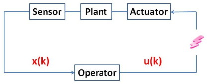
Figure 1: The closed-loop system

Replay attacks have been successfully used by the virus attack of Stuxnet [8, 18]. This class of attacks can be easily detected by attaching a time stamp to each control command. In the remainder of the paper, we assume that the attacks can always be detected and focus on the design and analysis of resilient controllers against them.

II-C Attack-resilient receding-horizon control law

Here we propose a variation of the receding-horizon control in; e.g. [17, 16], to deal with the replay attacks. Our attack-resilient receding-horizon control law, (for short, AR-RHC) is stated in Algorithm 1. In particular, at each time instant, the plant stores the whole control sequence which will be used in response to future attacks. The terminal state cost is chosen to coincide with the running state cost. This is instrumental for the analysis of performance degradation in Theorem II.1.

Algorithm 1 The attack-resilient receding-horizon control law

0:  The following steps are first performed by the operator:

1:  Choose $K$ so that $\sigma(\bar{A})$ is strictly inside the unit circle.

2:  Choose $\bar{Q}=\bar{Q}^{T}>0$ and obtain $\bar{P}$ by solving the following Lyapunov equation:

$$\bar{A}^{T}\bar{P}\bar{A}-\bar{P}=-\bar{Q}.$$ (2)

3:  Choose a constant $c>0$ such that $X_{0}\triangleq\{x\in\mathds{R}^{n}\;|\;\|x\|^{2}_{\bar{P}}\leq c\}\subseteq X$.

0:  At each $k\geq 0$, the operator, actuator and sensor execute the following steps:

1:  The operator solves the following $N$-horizon quadratic program, namely $N$-QP, parameterized by $x(k)\in X$:

$$\min_{\mathbf{u}(k)\in\mathds{R}^{m\times N}} \sum_{\tau=0}^{N-1}\big{(}\|x(k+\tau|k)\|^{2}_{P}+\|u(k+\tau|k)\|^{2}_{Q}\big{)}+\|x(k+N|k)\|^{2}_{P},$$

$${\rm{s.t.}} \quad x(k+\tau+1|k)=Ax(k+\tau|k)+Bu(k+\tau|k),$$

$$\quad x(k|k)=x(k),\quad x(k+\tau+1|k)\in X_{0},\quad u(k+\tau|k)\in U,\quad 0\leq\tau\leq N-1,$$

obtains the solution $\mathbf{u}(k)\triangleq[u(k|k),\cdots,u(k+N-1|k)]$, and sends it to the actuator.

2:  If $s(k)=0$, the actuator receives $\mathbf{u}(k)$, sets $M^{p}(k+1)=\mathbf{u}(k)$, implements $u(k|k)$, and the sensor sends $x(k+1)$ to the operator. If $s(k)\geq 1$, the actuator implements $u(k|k-s(k))$ in $M^{p}(k)$, sets $M^{p}(k+1)=M^{p}(k)$, and the sensor sends $x(k+1)$ to the operator.

3:  Repeat for $k=k+1$.

TABLE I: Main notations used in the following sections

$\lambda_{\textup{max}}(R)$ (resp. $\lambda_{\textup{min}}(R)$)	$\begin{array}[]{l}\text{the maximum (resp. minimum) eigenvalue of matrix $R$}\end{array}$
$\lambda\triangleq 1-\displaystyle{\frac{\lambda_{\textup{max}}(\bar{Q})}{\lambda_{\textup{min}}(\bar{P})}}$	$\begin{array}[]{l}\text{positive constant, $\lambda\in(0,1)$, see~{}\cite[cite]{[\@@bibref{}{TM-NF-MK:82}{}{}]},}\\ \text{defined with $\bar{Q}$, $\bar{P}$ introduced in AR-RHC}\end{array}$
$\phi_{N}\triangleq\displaystyle{\frac{\lambda_{\textup{max}}(\bar{P})\lambda_{\textup{max}}(P+K^{T}QK)}{\lambda_{\textup{min}}(\bar{P})}\frac{(1-\lambda^{N+1})}{1-\lambda}}$	$\begin{array}[]{l}\text{positive constant defined for all $N>0$,}\\ \text{with $\bar{Q}$, $\bar{P}$, and $K$ introduced in AR-RHC}\end{array}$
$\phi_{\infty}\triangleq\displaystyle{\frac{\lambda_{\textup{max}}(\bar{P})\lambda_{\textup{max}}(P+K^{T}QK)}{\lambda_{\textup{min}}(\bar{P})(1-\lambda)}}$	$\begin{array}[]{l}\text{positive constant defined with $\bar{Q}$, $\bar{P}$, and $K$ }\\ \text{introduced in AR-RHC}\end{array}$
$\alpha_{N}\triangleq\displaystyle{\frac{\lambda_{\textup{max}}(K^{T}QK+\bar{A}^{T}P\bar{A})}{\lambda_{\textup{min}}(P)}\times\prod_{\kappa=0}^{N-1}(1-\frac{\lambda_{\textup{min}}(P)}{\phi_{\kappa+1}})}$	$\begin{array}[]{l}\text{positive constant defined for all $N>0$,}\\ \text{with $\bar{A}$ and $K$ introduced in AR-RHC, and $\lambda$ introduced here}\end{array}$
$\rho_{N}\triangleq(1+\alpha_{N-1})(1-\frac{\lambda_{\textup{min}}(P)}{\phi_{N}})$	$\begin{array}[]{l}\text{a discount factor}\end{array}$
$W(x)\triangleq\|x\|^{2}_{\bar{P}}$	$\begin{array}[]{l}\text{matrix $\bar{P}$ is the solution to Lyapunov equation~{}\eqref{Ly-eq}}\end{array}$
$V_{N}$	$\begin{array}[]{l}\text{the optimal value function of $N$-QP}\end{array}$

In what follows, we present the results characterizing the stability and infinite-horizon cost induced by AR-RHC. See Table I, for the main notations employed, and Section V for the complete proof. Notice that the following property holds:

$$\frac{\lambda_{\textup{min}}(P)}{\phi_{N}}=\frac{\lambda_{\textup{min}}(P)}{\lambda_{\textup{max}}(P+K^{T}QK)}\frac{\lambda_{\textup{min}}(\bar{P})}{\lambda_{\textup{max}}(\bar{P})}\frac{(1-\lambda)}{(1-\lambda^{N+1})}<1.$$

where $\lambda$ and $\phi_{N}$ are defined in Table I. On the other hand, for $\alpha_{N}$ in Table I, $\alpha_{N}\searrow 0$ as $N\nearrow+\infty$, and $\phi_{N}$ is strictly increasing in $N$ and upper bounded by $\phi_{\infty}$. Then, given any integer $S\geq 1$, there is a smallest integer $N^{*}(S)\geq S$ such that for all $N\geq N^{*}(S)$, it holds that:

$$\gamma_{N,S}\triangleq(1-\frac{\lambda_{\textup{min}}(P)}{\phi_{\infty}})\max\{(1+\alpha_{N-S-1}),(1+\alpha_{N-1})\prod_{\ell=N-S}^{N-1}(1+\alpha_{\ell})\}<1.$$

Analogously, given any integer $S\geq 1$, there is a smallest integer $\hat{N}^{*}(S)\geq S$ such that for all $N\geq\hat{N}^{*}(S)$, it holds that

$$\hat{\gamma}_{N,S} \triangleq(1-\frac{\lambda_{\textup{min}}(P)}{\phi_{\infty}})^{2}(1+\alpha_{N-1})(1+\alpha_{N-2})$$

$$\times\big{(}\max_{s\in\{1,\cdots,S\}}\prod_{\ell=2}^{s}(1-\frac{\lambda_{\textup{min}}(P)}{\phi_{\infty}})(1+\alpha_{N-\ell-1})\big{)}\prod_{\ell=N-S}^{N-1}(1+\alpha_{\ell})<1.$$

One can easily verify $\hat{N}^{*}(S)\leq N^{*}(S)$. The following theorem characterizes the stability and infinite-horizon cost of system (1) under AR-RHC where $V_{\ell}(x)$ represents the value of the $\ell$-QP parameterized by $x\in X$.

Theorem II.1

(Stability and infinite-horizon cost) Let Assumptions II.1, II.2 and II.3 hold.

1. (Exponential stability) Suppose $N\geq\max\{N^{*}(S)+1,S+1\}$. Then system (1) under AR-RHC is exponentially stable when starting from $X_{0}$ with a rate of $\gamma_{N,S}$ in the sense that $V_{N-s(k-1)}(x(k))\leq\gamma_{N,S}^{k}V_{N}(x(0))$. In addition, the infinite-horizon cost of system (1) under AR-RHC is bounded above by $\frac{1}{1-\gamma_{N,S}}V_{N}(x(0))$.

2. (Asymptotic stability) If $N\geq\max\{\hat{N}^{*}(S)+1,S+1\}$, then system (1) under AR-RHC is asymptotically stable when starting from $X_{0}$.

Remark II.1

AR-RHC with Theorem II.1 can be readily extended to several scenarios, including DoS attacks, measurement attacks and the combinations of such attacks. If the adversary launches a DoS attack on control commands, the actuator receives nothing and then performs Step 3 in AR-RHC. The adversary may produce the replay attacks on the measurements sent from the sensor to the operator. If this happens, then the operator does not send anything to the actuator and the actuator performs Step 3 in AR-RHC. $\bullet$

III Discussion and simulations

III-A Extensions

AR-RHC with Theorem II.1 can be readily extended to several scenarios, including DoS attacks, measurement attacks and the combinations of such attacks. If the adversary launches a DoS attack on control commands, the actuator receives nothing and then performs Step 3 in AR-RHC. The adversary may produce the replay attacks on the measurements sent from the sensor to the operator. If this happens, then the operator does not send anything to the actuator and the actuator performs Step 3 in AR-RHC.

III-B Explicit upper bounds on $N^{*}(S)$ and $\hat{N}^{*}(S)$

Consider $S\geq 2$ and let $\chi\triangleq(1-\frac{\lambda_{\textup{min}}(P)}{\phi_{\infty}})$ and $\psi\triangleq\frac{\lambda_{\textup{max}}(K^{T}QK+\bar{A}^{T}P\bar{A})}{\lambda_{\textup{min}}(P)}$. Note that

$$\gamma_{N,S} \leq(1-\frac{\lambda_{\textup{min}}(P)}{\phi_{\infty}})(1+\alpha_{N-1})\prod_{\ell=N-S-1}^{N-1}(1+\alpha_{\ell})$$

$$\leq\chi(1+\alpha_{N-S-1})^{S+2}\leq\beta_{N,S}\triangleq\chi(1+\psi\chi^{N-S-1})^{S+2}.$$ (3)

So it suffices to find $N$ such that $\beta_{N,S}<1$. The relation $\beta_{N,S}<1$ is equivalent to the following:

$$N-S-1>\frac{\ln\big{(}\frac{1}{\psi}(\chi^{-\frac{1}{S+2}}-1)\big{)}}{\ln\chi}=\frac{\ln(\chi^{-\frac{1}{S+2}}-1)-\ln\psi}{\ln\chi}.$$

Hence, an explicit upper bound on $N^{*}(S)$ is $\Pi_{E}(S)\triangleq S+1+\frac{\ln(\chi^{-\frac{1}{S+2}}-1)-\ln\psi}{\ln\chi}$.

We now move to find an explicit upper bound on $\hat{N}^{*}(S)$. Note that

$$\hat{\gamma}_{N,S} \leq(1-\frac{\lambda_{\textup{min}}(P)}{\phi_{\infty}})^{2}(1+\alpha_{N-1})(1+\alpha_{N-2})\big{(}\max_{s\in\{1,\cdots,S\}}\prod_{\ell=2}^{s}(1-\frac{\lambda_{\textup{min}}(P)}{\phi_{\infty}})(1+\alpha_{N-\ell-1})\big{)}\prod_{\ell=N-S}^{N-1}(1+\alpha_{\ell})$$

$$\leq(1-\frac{\lambda_{\textup{min}}(P)}{\phi_{\infty}})^{S+1}(1+\alpha_{N-1})(1+\alpha_{N-2})(1+\alpha_{N-S-1})^{S-1}\prod_{\ell=N-S}^{N-1}(1+\alpha_{\ell})$$

$$\leq(1-\frac{\lambda_{\textup{min}}(P)}{\phi_{\infty}})^{S+1}(1+\alpha_{N-S-1})^{2S+1}=\chi^{S+1}(1+\psi\chi^{N-S-1})^{2S+1}.$$

So, an explicit upper bound on $\hat{N}^{*}(S)$ is $\Pi_{A}(S)\triangleq S+1+\frac{\ln(\chi^{-\frac{S+1}{2S+1}}-1)-\ln\psi}{\ln\chi}$. This pair of upper bounds clearly demonstrate that a higher computational complexity; i.e., a larger $N$, is caused by a larger $S$, indicating that the adversary is less energy constrained. On the other hand, the second term in $\Pi_{A}(S)$ approaches a constant as $S$ goes to infinity. So $\Pi_{A}(S)$ can be upper bounded by an affine function. However, the second term in $\Pi_{E}(S)$ dominates when $S$ is large. That is, exponential stability demands a much higher cost than asymptotic stability when $S$ is large.

III-C A reverse scenario

Reciprocally, for any horizon $N\geq 1$, there is a largest integer $S^{*}(N)\leq N-1$ (resp. $\hat{S}^{*}(N)\leq N-1$) such that for all $S\leq S^{*}(N)$ (resp. $S\leq\hat{S}^{*}(N)$), it holds that $\gamma_{N,S}<1$ (resp. $\hat{\gamma}_{N,S}<1$). Theorem II.1 still applies to this reverse scenario and characterizes the “security level” or “amount of resilience” that the proposed receding-horizon control algorithm possesses.

III-D Optimal resilience management

The analysis of Theorem II.1 quantifies the cost and constraints that allow the AR-RHC algorithm to work despite consecutive attacks under limited computation capabilities. These metrics can be used for optimal resilience management of a network as follows.

As [3], we consider a set of players $V\triangleq\{1,\cdots,N\}$ where the players share a communication network and each of them is associated with a decoupled dynamic system:

$$x_{i}(k+1)=A_{i}x_{i}(k)+B_{i}u_{i}(k).$$ (4)

Each player $i$ implements his own AR-RHC with horizon $N_{i}$. The notations in the previous sections can be defined analogously for each player and the set of the notations of player $i$ will be indexed by $i$.

By (3), we associate player $i$ with the following cost function:

$$\mathcal{C}_{i}(M)=\big{(}1+\psi_{i}\chi_{i}^{N_{i}-\mathcal{S}(\textbf{1}^{T}M)}\big{)}^{\mathcal{S}(\textbf{1}^{T}M)+1}+\frac{1}{2}a_{i}M_{i}^{2},$$ (5)

where $M_{i}\in[M_{i,\min},M_{i,\max}]\subset\mathds{R}_{>0}$ is the security investment of player $i$, $a_{i}\in\mathds{R}_{>0}$ is a weight on the security cost the and 1 is the vector with $N$ ones. The non-negative real value $\mathcal{S}(\textbf{1}^{T}M)$ represents the security level given the investment vector $M$ of all players, where $\mathcal{S}:\mathds{R}_{\geq 0}\rightarrow\mathds{R}_{\geq 0}$ is convex, non-decreasing, and smooth. We assume that each player has a fixed computational power, and so $N_{i}$ is fixed. The players need to make the investment such that

$$\mathcal{S}(\textbf{1}^{T}M)\leq\min_{i\in V}S_{i}^{*}(N_{i}).$$ (6)

Remark III.1

Note that $S$ is an integer in (3). In (5) and (6), we use the real value of $\mathcal{S}(\textbf{1}^{T}M)$ as an approximation. $\bullet$

We now compute the first-order partial derivative of $\mathcal{C}_{i}$ as follows:

$$\frac{\partial\mathcal{C}_{i}}{\partial M_{i}} =-\ln(1+\psi_{i}\chi_{i}^{N_{i}-\mathcal{S}(\textbf{1}^{T}M)})(1+\psi_{i}\chi_{i}^{N_{i}-\mathcal{S}(\textbf{1}^{T}M)})^{\mathcal{S}(\textbf{1}^{T}M)+1}(\ln\chi_{i})\psi_{i}\chi_{i}^{N_{i}-\mathcal{S}_{i}(M)}(\frac{\partial\mathcal{S}}{\partial y})^{2}+a_{i}M_{i}$$

where we use the shorthand $y\triangleq\textbf{1}^{T}M$. With this, we further derive the second-order partial derivative as follows:

$$\frac{\partial^{2}\mathcal{C}_{i}}{\partial M_{i}^{2}} =\psi_{i}^{2}(\ln\chi_{i})^{2}\chi_{i}^{2(N_{i}-\mathcal{S}_{i}(\textbf{1}^{T}M))}(1+\psi_{i}\chi_{i}^{N_{i}-\mathcal{S}(\textbf{1}^{T}M)})^{\mathcal{S}(\textbf{1}^{T}M)}(\frac{\partial\mathcal{S}}{\partial y})^{3}+a_{i}$$

$$+(\ln(1+\psi_{i}\chi_{i}^{N_{i}-\mathcal{S}(\textbf{1}^{T}M)}))^{2}(1+\psi_{i}\chi_{i}^{N_{i}-\mathcal{S}(\textbf{1}^{T}M)})^{\mathcal{S}(\textbf{1}^{T}M)+1}(\psi_{i}\ln\chi_{i}\chi_{i}^{N_{i}-\mathcal{S}_{i}(\textbf{1}^{T}M)})^{2}(\frac{\partial\mathcal{S}}{\partial y})^{4}$$

$$+\ln(1+\psi_{i}\chi_{i}^{N_{i}-\mathcal{S}(\textbf{1}^{T}M)})(1+\psi_{i}\chi_{i}^{N_{i}-\mathcal{S}(\textbf{1}^{T}M)})^{\mathcal{S}(\textbf{1}^{T}M)+1}\psi_{i}(\ln\chi_{i})^{2}\chi_{i}^{N_{i}-\mathcal{S}_{i}(\textbf{1}^{T}M)}(\frac{\partial\mathcal{S}}{\partial y})^{3}$$

$$+2(\ln(1+\psi_{i}\chi_{i}^{N_{i}-\mathcal{S}(\textbf{1}^{T}M)}))^{2}(1+\psi_{i}\chi_{i}^{N_{i}-\mathcal{S}(\textbf{1}^{T}M)})^{\mathcal{S}(\textbf{1}^{T}M)+1}\psi_{i}(-\ln\chi_{i})\chi_{i}^{N_{i}-\mathcal{S}_{i}(\textbf{1}^{T}M)}\frac{\partial\mathcal{S}}{\partial y}\frac{\partial^{2}\mathcal{S}}{\partial y^{2}}.$$

Recall that $\chi_{i}\in(0,1]$ and $\mathcal{S}$ is non-decreasing and convex. So $\frac{\partial^{2}\mathcal{C}_{i}}{\partial M_{i}^{2}}\geq 0$ and $\mathcal{C}_{i}$ is convex in $M_{i}$. Analogously, one can show that $\mathcal{C}_{i}$ is convex in $M$.

III-D1 Competitive resource allocation scenario

Consider a resilience management game, where each player $i$ minimizes his cost $\mathcal{C}_{i}(M)$, subject to the common constraint (6) and his private constraint $M_{i}\in[M_{i,\min},M_{i,\max}]\subset\mathds{R}_{>0}$. Since $\mathcal{C}_{i}$ and $\mathcal{S}$ are convex in $M_{i}$, then the game is a generalized convex game. The distributed algorithms in [31] can be directly utilized to numerically compute a Nash equilibrium of the resilience management game, and the algorithms in [31] are able to tolerate transmission delays and packet dropouts.

Remark III.2

The paper [3] considers a set of identical and independent networked control systems and each of them aims to solve an infinite-horizon LQG problem. The authors study a different security game where the decisions of each player are binary, participating in the security investment or not. $\bullet$

III-D2 Cooperative resource allocation scenario

Consider a resilience management optimization problem, where the players aim to collectively minimize $\sum_{i\in V}\mathcal{C}_{i}(M)$, subject to the global constraint (6) and the private constraint $M_{i}\in[M_{i,\min},M_{i,\max}]\subset\mathds{R}_{>0}$. Since $\mathcal{C}_{i}$ and $\mathcal{S}$ are convex, then the problem is a convex program. The distributed algorithms in [34] can be directly exploited to numerically compute a global minimizer of this problem, and the algorithms in [34] are robust to the dynamic changes of inter-player topologies.

III-E Simulations

In this section, we provide a numerical example to illustrate the performance of our algorithm. The set of system parameters are given as follows:

$$A=\left[\begin{array}[]{cc}2&1\\ 1&2\end{array}\right],\quad B=\left[\begin{array}[]{c}2\\ 1\end{array}\right],\quad K=[-3.25\;\;-3],\quad P=I,\quad Q=1,$$

$$\bar{Q}=I,\quad\bar{P}=\left[\begin{array}[]{cc}25.6667&13.3333\\ 13.3333&8.2963\end{array}\right],\quad c=100,\quad u_{\max}=500.$$

Figure 2 shows the temporal evolution of $\|x(k)\|^{2}$ under three attacking horizons $S=0,2,5$. One can see that a larger $S$ induces a longer time to converge, and larger oscillation before reaching the equilibrium. In our simulations, a smaller horizon $N=15$ than the one determined theoretically is already sufficient to achieve system stabilization.

Figure 2: The trajectories of $\|x(k)\|^{2}$ under the attack-resilient receding-horizon control algorithm

IV Conclusions

In this paper, we have studied a resilient control problem where a linear dynamic system is subject to the replay and DoS attacks. We have proposed a variation of the receding-horizon control law for the operator and analyzed system stability and performance degradation. We have also studied a class of competitive (resp. cooperative) resource allocation problems for resilient networked control systems. Extension to multi-agent systems will be considered in the future.

V Appendix: Technical proofs

The proofs toward Theorem II.1 are collected in this section. In particular, the proofs for the intermediate lemmas are based on the corresponding results in our previous paper [33] on deception attacks. The proofs for the main theorem are new and not included in [33]. In the proof of Theorem II.1, we choose $V_{N-s(k-1)}(x(k))$ as a Lyapunov function candidate. To analyze its convergence, we first establish several instrumental properties of $V_{N}$, including monotonicity, diminishing rations with respect to $N$ and decreasing property.

Recall the definitions of $\lambda$, $\alpha_{N}$, $\phi_{N}$, and $\phi_{\infty}$ summarized in Table I. It follows from [20] that $\lambda\in(0,1)$, and clearly, $1\leq\phi_{N}\leq\phi_{\infty}$ for any $N\in{\mathbb{Z}}_{>0}$. Observe that the following holds for any $\kappa\in{\mathbb{Z}}_{>0}$:

$$\frac{\lambda_{\textup{min}}(P)}{\phi_{\kappa+1}}=\frac{\lambda_{\textup{min}}(P)}{\lambda_{\textup{max}}(P+K^{T}QK)}\frac{\lambda_{\textup{min}}(\bar{P})}{\lambda_{\textup{max}}(\bar{P})}\frac{1-\lambda}{1-\lambda^{{\kappa}+2}}\geq\frac{\lambda_{\textup{min}}(P)}{\lambda_{\textup{max}}(P+K^{T}QK)}\frac{\lambda_{\textup{min}}(\bar{P})}{\lambda_{\textup{max}}(\bar{P})}(1-\lambda)\in(0,1).$$

This ensures the monotonicity of $\alpha_{N}$ and, moreover, that $\alpha_{N}\searrow 0$ as $N\nearrow+\infty$.

We show the forward invariance property of system (1) in $X_{0}$ under $Kx$.

Lemma V.1 (Forward invariance in $X_{0}$)

The set $X_{0}$ is forward invariant for system (1) under the auxiliary controller $Kx$ with the control constraint $U$; i.e., for any $x\in X_{0}$, it holds that $u=Kx\in U$ and $\bar{A}x\in X_{0}$.

Proof:

The differences of $W$ along the trajectories of the dynamics (1) under $u(k)=Kx(k)$, $x(k)=x$ can be characterized by:

$$W(x(k+1))-W(x)=\|\bar{A}x(k+1)\|^{2}_{\bar{P}}-\|x(k)\|^{2}_{\bar{P}}=-\|x\|^{2}_{\bar{Q}}\leq-\lambda_{\textup{min}}(\bar{Q})\|x\|^{2},$$ (7)

where $W(x)$, $\bar{A}$, $\bar{P}$ and $\bar{Q}$ are given in Table I, and in the second equality we apply the Lyapunov equation (2). Since $\bar{Q}>0$, then $W(x(k+1))\leq W(x)$. Since $x$ belongs to $X_{0}$, so does $x(k+1)$. Since $X_{0}\subseteq X$, we know that $u(k)\in U$ by Assumption II.2. The forward invariance property of $X_{0}$ for system (1) follows. ∎

On the other hand, one can see that the $N$-QP parameterized by $x\in X_{0}$ has at least one solution generated by the auxiliary controller.

Lemma V.2 (Feasibility of the $N$-QP)

For any $x\in X_{0}$, consider system (1) with $x(k|k)=x$ and $u(k+\tau|k)=Kx(k+\tau|k)$, for $0\leq\tau\leq N-1$. Then, ${\mathbf{u}}(k)$ is a feasible solution to the $N$-QP parameterized by $x(k)\in X_{0}$.

Proof:

It is a direct result of Lemma V.1 and Assumption II.2. ∎

The following lemma demonstrates that $V_{N}$ is bounded above and below by two quadratic functions, respectively.

Lemma V.3

(Positive-definite and decrescent properties of $V_{N}$) The function $V_{N}$ is quadratically bounded above and below as $\lambda_{\textup{min}}(P)\|x\|^{2}\leq V_{N}(x)\leq\phi_{N}\|x\|^{2}$ for any $x\in X_{0}$.

Proof:

Consider any $x\in X_{0}$. It is easy to see that $V_{N}(x)\geq\lambda_{\textup{min}}(P)\|x\|^{2}$, and thus positive definiteness of $V_{N}$ follows. We now proceed to show that $V_{N}$ is decrescent. In order to simplify the notations in the proof, we will drop the dependency on time $k$ in what follows. Toward this end, we let $\{x(\tau)\}_{\tau\geq 0}$ be the solution produced by the system $x(\tau+1)=\bar{A}x(\tau)$, that is, the closed-loop system solution of the dynamics (1) under the auxiliary controller $Kx$, with initial state $x(0)=x\in X_{0}$. We denote $x(\tau|0)\equiv x(\tau)$ and $u(\tau|0)\equiv u(\tau)$. Recall the estimate (7):

$$W(x(\tau+1)) \leq W(x(\tau))-\lambda_{\textup{min}}(\bar{Q})\|x(\tau)\|^{2}\leq W(x(\tau))-\frac{\lambda_{\textup{max}}(\bar{Q})}{\lambda_{\textup{max}}(\bar{P})}W(x(\tau)),$$ (8)

where we use the property that $\lambda_{\textup{min}}(\bar{P})\|x\|^{2}\leq W(x)\leq\lambda_{\textup{max}}(\bar{P})\|x\|^{2}$. It follows from Lemma V.2 that the sequence of control commands $u(\tau)=Kx(\tau)$ for $0\leq\tau\leq N-1$ consists of a feasible solution to the $N$-QP parameterized by $x\in X_{0}$. Then we achieve the following on $V_{N}(x)$:

$$V_{N}(x) \leq\sum_{\tau=0}^{N-1}\big{(}\|x(\tau)\|^{2}_{P}+\|Kx(\tau)\|^{2}_{Q}\big{)}+\|x(N)\|^{2}_{P}$$

$$\leq\sum_{\tau=0}^{N-1}\lambda_{\textup{max}}(P+K^{T}QK)\|x(\tau)\|^{2}+\lambda_{\textup{max}}(P)\|x(N)\|^{2}$$

$$\leq\frac{\lambda_{\textup{max}}(P+K^{T}QK)}{\lambda_{\textup{min}}(\bar{P})}\sum_{\tau=0}^{N-1}W(x(\tau))+\frac{\lambda_{\textup{max}}(P)}{\lambda_{\textup{min}}(\bar{P})}W(x(N)).$$ (9)

Substituting inequality (8) into (9), we obtain the following estimates on $V_{N}(x)$:

$$V_{N}(x) \leq\frac{\lambda_{\textup{max}}(P+K^{T}QK)}{\lambda_{\textup{min}}(\bar{P})}W(x)\sum_{\tau=0}^{N-1}\lambda^{\tau}+\frac{\lambda_{\textup{max}}(P)}{\lambda_{\textup{min}}(\bar{P})}W(x)\lambda^{N}$$

$$\leq\frac{\lambda_{\textup{max}}(\bar{P})\lambda_{\textup{max}}(P+K^{T}QK)}{\lambda_{\textup{min}}(\bar{P})}\frac{1-\lambda^{N+1}}{1-\lambda}\|x\|^{2}.$$

where we use the fact $\lambda=1-\frac{\lambda_{\textup{max}}(\bar{Q})}{\lambda_{\textup{max}}(\bar{P})}\in(0,1)$ in [20]. The decrescent property of $V_{N}$ immediately follows from the above relations. ∎

Next, one can show that for any $x\in X_{0}$, $V_{N}(x)$ does not decrease as $N$ increases.

Lemma V.4 (Monotonicity of $V_{N}$)

The optimal value function $V_{N}$ is monotonic in $N$; i.e., for any $x\in X_{0}$, $V_{N^{\prime}}(x)\leq V_{N}(x)$ for $N^{\prime}<N$.

Proof:

Consider $N^{\prime}<N$, and denote by $J_{N}$ and $J_{N^{\prime}}$ the objective functions of the $N$-QP and the $N^{\prime}$-QP, respectively. Let ${\mathbf{u}}_{N}$ be a solution to the $N$-QP parameterized by $x$, with $\mathbf{u}_{N}=[u(0),\dots,u(N-1)]$, and let ${\mathbf{u}}_{N^{\prime}}$, with $\mathbf{u}_{N^{\prime}}=[u(0),\dots,u(N^{\prime}-1)]$, be a solution to the ${N^{\prime}}$-QP parameterized by $x\in X_{0}$. We construct $\tilde{{\mathbf{u}}}_{N^{\prime}}\in U^{N^{\prime}}$, a truncated version of ${\mathbf{u}}_{N}$, in such a way that $\tilde{u}(k)=u(k)$ for $0\leq k\leq{N^{\prime}}-1$. Since ${\mathbf{u}}_{N}$ is a solution to the $N$-QP parameterized by $x$, then one can show that $\tilde{\mathbf{u}}_{N^{\prime}}$ is a feasible solution to the ${N^{\prime}}$-QP parameterized by $x$. This renders the following upper bound on $V_{N^{\prime}}(x)$:

$$V_{N^{\prime}}(x)=J_{N^{\prime}}(x,{\mathbf{u}}_{N^{\prime}})\leq J_{N^{\prime}}(x,\tilde{\mathbf{u}}_{N^{\prime}}).$$ (10)

Denote by $\mathbf{x}_{N}\triangleq[x(0),\cdots,x(N)]$ the corresponding trajectory to $\mathbf{u}_{N}$ with initial state $x(0)=x$ and by $\tilde{\mathbf{x}}_{N^{\prime}}\triangleq[\tilde{x}(0),\cdots,\tilde{x}_{N^{\prime}}]$ the corresponding trajectory generated by the sequence of $\tilde{{\mathbf{u}}}_{N^{\prime}}$ with the initial state $\tilde{x}(0)=x$. Since $\tilde{{\mathbf{u}}}_{N^{\prime}}$ is a truncated version of ${\mathbf{u}}_{N}$, we have that $\tilde{x}(k)=x(k)$ for $0\leq k\leq N^{\prime}$. Denote further $\tilde{\mathbf{u}}_{N^{\prime}}\triangleq[\tilde{u}(0),\cdots,\tilde{u}(N^{\prime}-1)]$. Then we have

$$J_{N^{\prime}}(x,\tilde{{\mathbf{u}}}_{N^{\prime}})=\sum_{k=1}^{{N^{\prime}}}\big{(}\|\tilde{x}(k)\|^{2}_{P}+\|\tilde{u}(k)\|^{2}_{Q}\big{)}+\|\tilde{x}(N^{\prime})\|^{2}_{P}$$

$$=\sum_{k=1}^{{N^{\prime}}}\big{(}\|x(k)\|^{2}_{P}+\|u(k)\|^{2}_{Q}\big{)}+\|x(N^{\prime})\|^{2}_{P}\leq\sum_{k=1}^{N}\big{(}\|x(k)\|^{2}_{P}+\|u(k)\|^{2}_{Q}\big{)}+\|x(N)\|^{2}_{P}=V_{N}(x).$$

The combination of (10) and the above relation establishes that $V_{N^{\prime}}(x)\leq V_{N}(x)$ for $x\in X_{0}$. ∎

The following lemma formalizes that for any $x\in X_{0}$, the difference between $V_{N+1}(x)$ and $V_{N}(x)$ decreases as $N$ increases by noting that $V_{N}(x)\leq V_{N+1}(x)$ and $\alpha_{N}$ is strictly decreasing in $N$, where $V_{N+1}$ and $V_{N}$ are the optimal value functions for the $(N+1)$-QP and the $N$-QP, respectively. This property is referred to as the property of diminishing ratios of $V_{N}$ in $N$ by noting that $\alpha_{N}\searrow 0$ as $N\nearrow+\infty$.

Lemma V.5

(The diminishing ratios of $V_{N}$ in $N$) The optimal value function $V_{N}$ is diminishingly increasing in $N$ in such a fashion that $\frac{V_{N+1}(x)-V_{N}(x)}{V_{N}(x)}\leq\alpha_{N}$ for any $x\in X_{0}$.

Proof:

Let ${\mathbf{u}}_{N}$, with $\mathbf{u}_{N}=[u(0),\dots,u(N-1)]$, be a solution to the $N$-QP parameterized by $x\in X_{0}$. Let $\mathbf{x}_{N}=[x(0),\dots,x(N)]$, $x(0)=x$, be the corresponding trajectory. Notice that $x(k)\in X_{0}$ for $0\leq k\leq N$. We construct an extended version $\tilde{\mathbf{u}}_{N+1}\in U^{N+1}$ of ${\mathbf{u}}_{N}$ as $\tilde{\mathbf{u}}_{N+1}=[u(0),\dots,u(N-1),Kx(N)]$. Since $x(N)\in X_{0}$, then $\tilde{x}(N+1):=\bar{A}x(N)\in X_{0}$ by Lemma V.1, implying that $\tilde{\mathbf{u}}_{N+1}$ consists of a feasible solution to the $(N+1)$-QP parameterized by $x$. Then we establish the following upper bounds on $V_{N+1}(x)$:

$$V_{N+1}(x)\leq J_{N+1}(x,\tilde{\mathbf{u}}_{N+1})=J_{N}(x,{\mathbf{u}}_{N})+\|Kx(N)\|^{2}_{Q}+\|\tilde{x}(N+1)\|_{P}^{2}\leq V_{N}(x)+\varsigma\|x(N)\|^{2},$$ (11)

where $\varsigma:=\lambda_{\textup{max}}(K^{T}QK+\bar{A}^{T}P\bar{A})$. We now turn our attention to find a relation between $\|x(N)\|^{2}$ and $V_{N}(x)$. To achieve this, we will show the following holds for $\ell\in\{0,\cdots,N\}$ by induction:

$$V_{\ell}(x(N-\ell))\leq\prod_{\kappa=\ell}^{N-1}(1-\frac{\lambda_{\textup{min}}(P)}{\phi_{\kappa+1}})V_{N}(x).$$ (12)

It follows from Bellman’s principle of optimality that

$$V_{N}(x)=\|x(0)\|_{P}^{2}+\|u(0)\|^{2}_{Q}+V_{N-1}(x(1)).$$

We can further see that $V_{N}(x)-V_{N-1}(x(1))$ is lower bounded in the following way:

$$V_{N}(x)-V_{N-1}(x(1))\geq\lambda_{\textup{min}}(P)\|x\|^{2}\geq\frac{\lambda_{\textup{min}}(P)}{\phi_{N}}V_{N}(x),$$ (13)

where we use the decrescent property in Lemma V.3 in the last inequality. Rearrange terms in (13) and it renders that (12) holds for $\ell=N-1$.

Assume that (12) holds for some $\ell+1\in\{1,\cdots,N-1\}$; i.e., the following holds:

$$V_{\ell+1}(x(N-\ell-1))\leq\prod_{\kappa=\ell+1}^{N-1}(1-\frac{\lambda_{\textup{min}}(P)}{\phi_{\kappa+1}})V_{N}(x).$$ (14)

Similar to (13), it follows from Bellman’s principle of optimality and Lemma V.3 that

$$V_{\ell+1}(x(N-\ell-1))-V_{\ell}(x(N-\ell))\geq\lambda_{\textup{min}}(P)\|x(N-\ell-1)\|^{2}\geq\frac{\lambda_{\textup{min}}(P)}{\phi_{\ell+1}}V_{\ell+1}(x(N-\ell-1)).$$ (15)

Combining (14) and (15) renders that

$$V_{\ell}(x(N-\ell))\leq(1-\frac{\lambda_{\textup{min}}(P)}{\phi_{\ell+1}})V_{\ell+1}(x(N-\ell-1))\leq\prod_{\kappa=\ell}^{N-1}(1-\frac{\lambda_{\textup{min}}(P)}{\phi_{\kappa+1}})V_{N}(x).$$

This implies (12) holds for $\ell$. By induction, we conclude that (12) holds for $\ell\in\{0,\cdots,N\}$. Let $\ell=0$ in (12), and we have that $V_{0}(x(N))\leq\prod_{\kappa=0}^{N-1}(1-\frac{\lambda_{\textup{min}}(P)}{\phi_{\kappa+1}})V_{N}(x)$, implying that $\|x(N)\|^{2}\leq\frac{1}{\lambda_{\textup{min}}(P)}\prod_{\kappa=0}^{N-1}(1-\frac{\lambda_{\textup{min}}(P)}{\phi_{\kappa+1}})V_{N}(x)$ by Lemma V.3. By combining this relation with (11), we obtain the desired relation between $V_{N+1}$ and $V_{N}$. ∎

A relation between $V_{N}(x(k+1|k))$ and $V_{N}(x(k))$ for $x(k)\in X_{0}$, and $x(k+1|k)$ generated through the $N$-QP, is found next.

Lemma V.6 (Decreasing property of $V_{N}$ in $X_{0}$)

With $x(k+1|k)$ generated through the $N$-QP starting from $x(k)$, the following decreasing property holds for any $x(k)\in X_{0}$:

$$V_{N}(x(k+1|k))\leq\rho_{N}V_{N}(x(k)).$$

Proof:

With Lemma V.3 and V.5, we reach the following relation between $V_{N}(x(k+1|k))$ and $V_{N}(x(k))$ for any $x(k)\in X_{0}$:

$$V_{N}(x(k+1|k))\leq(1+\alpha_{N-1})V_{N-1}(x(1))\leq(1+\alpha_{N-1})(V_{N}(x(k))-\|x(k)\|_{P}^{2})$$

$$\leq(1+\alpha_{N-1})(V_{N}(x(k))-\lambda_{\textup{min}}(P)\|x(k)\|^{2})\leq(1+\alpha_{N-1})(1-\frac{\lambda_{\textup{min}}(P)}{\phi_{N}})V_{N}(x(k)),$$

where Lemma V.5 and Lemma V.3 are used in the first and last inequalities, respectively, by noting that $x(k+1|k)$ and $x(k)$ in $X_{0}$. ∎

Proof of Theorem II.1:

Proof:

[Part 1: Exponential stability] Let us consider the first part of $N\geq\max\{N^{*}(S)+1,S+1\}$. Recall that $x(0)\in X_{0}$ and the state constraint $X_{0}$ is enforced in the $N$-QP. Repeatedly apply Lemma V.2 and we have that $x(k)\in X_{0}$ for all $k\geq 0$. We now distinguish four cases:

Case 1: $\vartheta(k)=1$ and $\vartheta(k-1)=0$. For this case, $s(k)=1$, $s(k-1)=0$, and we have

$$V_{N-s(k)}(x(k+1))=V_{N-1}(x(k+1))\leq\rho_{N-1}V_{N-1}(x(k))$$

$$\leq\rho_{N-1}V_{N}(x(k))=\rho_{N-1}V_{N-s(k-1)}(x(k)),$$

where the first inequality uses Lemma V.6 and the principle of optimality, and the second one exploits Lemma V.4.

Case 2: $\vartheta(k)=\vartheta(k-1)=0$. Here, $s(k)=s(k-1)=0$. By Lemma V.6, we have

$$V_{N-s(k)}(x(k+1))=V_{N}(x(k+1))\leq\rho_{N}V_{N}(x(k))=\rho_{N}V_{N-s(k-1)}(x(k)).$$

Case 3: $\vartheta(k)=\vartheta(k-1)=1$. Note that $s(k)=s(k-1)+1$, and then

$$V_{N-s(k)}(x(k+1))\leq\rho_{N-s(k)}V_{N-s(k)}(x(k))\leq\rho_{N-s(k)}V_{N-s(k-1)}(x(k)),$$

where the first inequality utilizes Lemmas V.6 and the principle of optimality, and the second one exploits Lemma V.4.

Case 4: $\vartheta(k)=0$ and $\vartheta(k-1)=1$. For this case, we have $s(k)=0$, $s(k-1)\geq 1$ and thus

$$V_{N-s(k)}(x(k+1))=V_{N}(x(k+1))\leq\rho_{N}V_{N}(x(k))\leq\rho_{N}\prod_{\ell=N-s(k-1)}^{N-1}(1+\alpha_{\ell})V_{N-s(k-1)}(x(k)),$$

where the last inequality repeatedly applies Lemma V.5.

Combine the above four cases, and it renders the following:

$$V_{N-s(k)}(x(k+1)) \leq\max\{\max_{s\in\{1,\cdots,S\}}\{\rho_{N-s}\},\rho_{N}\max_{s=1,\cdots,S}\{\prod_{\ell=N-s}^{N-1}(1+\alpha_{\ell})\}\}V_{N-s(k-1)}(x(k))$$

$$\leq\gamma_{N,S}V_{N-s(k-1)}(x(k)).$$ (16)

Since $0<\gamma_{N,S}<1$, $\{V_{N-s(k-1)}(x(k))\}$ exponentially diminishes, and the following holds:

$$V_{N-s(k-1)}(x(k))\leq\gamma_{N,S}^{k}V_{N}(x(0)).$$ (17)

Recall $N\geq S+1$. It follows from (17) that the infinite-horizon cost is characterized as follows:

$$\sum_{k=0}^{+\infty}(\|x(k)\|_{P}^{2}+\|u(k)\|_{Q}^{2})\leq\sum_{k=0}^{+\infty}V_{N-s(k-1)}(x(k))\leq\sum_{k=0}^{+\infty}\gamma_{N,S}^{k}V_{N}(x(0))=\frac{1}{1-\gamma_{N,S}}V_{N}(x(0)).$$

We then have finished the proofs for the first part.

[Part 2: Asymptotic stability] We now proceed to show the second part of $N\geq\max\{\hat{N}^{*}(S)+1,S+1\}$. Towards this end, we partition the time horizon $\{0,1,\cdots\}$ into a sequence of subsets $\{C_{1},A_{1},C_{2},A_{2},\cdots\}$ where $C_{i}=\{c_{i}^{L},\cdots,c_{i}^{U}\}$ and $A_{i}=\{a_{i}^{L},\cdots,a_{i}^{U}\}$ with for $k\in C_{i}$, then $\vartheta(k)=0$; and $k\in A_{i}$, then $\vartheta(k)=1$. Note that $c_{0}^{L}=0$ and $a_{i}^{L}=c_{i}^{U}+1$.

Case 1: $k\in C_{i}\setminus\{c_{i}^{L}\}$. Note that $s(k)=s(k-1)=0$ for all $k\in C_{i}\setminus\{c_{i}^{L}\}$. By Lemma V.6, we have

$$V_{N-s(k)}(x(k+1))\leq\rho_{N}V_{N-s(k-1)}(x(k)),\quad\forall k\in C_{i}\setminus\{c_{i}^{L}\}.$$

Case 2: $k=a_{i}^{L}$. Note that $\vartheta(a_{i}^{L})=1$ and $\vartheta(a_{i}^{L}-1)=0$. By Case 1 in Part 1, we have

$$V_{N-s(a_{i}^{L})}(x(a_{i}^{L}+1))\leq\rho_{N-1}V_{N-s(a_{i}^{L}-1)}(x(a_{i}^{L})).$$

Case 3: $k=A_{i}\setminus\{a_{i}^{L}\}$. Recall that $\vartheta(k)=1$ for $k\in A_{i}$. By repeating the result of Case 3 in Part 1, we have

$$V_{N-s(k)}(x(k+1))\leq\prod_{\ell=2}^{k-a_{i}^{L}}\rho_{N-\ell}V_{N-s(a_{i}^{L})}(x(a_{i}^{L}+1)),\quad\forall k\in A_{i}\setminus\{a_{i}^{L}\}.$$

Case 4: $k=c_{i+1}^{L}=a_{i}^{U}+1$. Note that $\vartheta(c_{i+1}^{L})=0$ and $\vartheta(c_{i+1}^{L}-1)=1$. By Case 4 in Part 1, it holds that

$$V_{N-s(c_{i+1}^{L})}(x(c_{i+1}^{L}+1))\leq\rho_{N}\prod_{\ell=N-s(c_{i+1}^{L}-1)}^{N-1}(1+\alpha_{\ell})V_{N-s(c_{i+1}^{L}-1)}(x(c_{i+1}^{L})).$$

The combination of the above four relations renders the following:

$$V_{N-s(c_{i+1}^{L})}(x(c_{i+1}^{L}+1)) \leq\rho_{N}\prod_{\ell=N-s(c_{i+1}^{L}-1)}^{N-1}(1+\alpha_{\ell})V_{N-s(c_{i+1}^{L}-1)}(x(c_{i+1}^{L}))$$

$$=\rho_{N}\prod_{\ell=N-s(c_{i+1}^{L}-1)}^{N-1}(1+\alpha_{\ell})V_{N-s(c_{i+1}^{L}-1)}(x(a_{i}^{U}+1))$$

$$\leq\rho_{N}\prod_{\ell=2}^{a_{i}^{U}-a_{i}^{L}}\rho_{N-\ell}\prod_{\ell=N-s(c_{i+1}^{L}-1)}^{N-1}(1+\alpha_{\ell})V_{N-s(c_{i+1}^{L}-1)}(x(a_{i}^{L}+1))$$

$$\leq\rho_{N}\rho_{N-1}\prod_{\ell=2}^{a_{i}^{U}-a_{i}^{L}}\rho_{N-\ell}\prod_{\ell=N-s(c_{i+1}^{L}-1)}^{N-1}(1+\alpha_{\ell})V_{N-s(c_{i+1}^{L}-1)}(x(a_{i}^{L}))$$

$$=\rho_{N}\rho_{N-1}\prod_{\ell=2}^{a_{i}^{U}-a_{i}^{L}}\rho_{N-\ell}\prod_{\ell=N-s(c_{i+1}^{L}-1)}^{N-1}(1+\alpha_{\ell})V_{N-s(c_{i+1}^{L}-1)}(x(c_{i}^{U}+1))$$

$$\leq\hat{\gamma}_{N,S}V_{N-s(c_{i+1}^{L}-1)}(x(c_{i}^{L})),$$

where the four inequalities sequentially apply Cases 4 to 1. Since $\hat{\gamma}_{N,S}\in(0,1)$, the subsequence $\{V_{N-s(c_{i+1}^{L}-1)}(x(c_{i+1}^{L}))\}$ exponentially decreases.

By the above four cases, it is not difficult to verify that the following holds for all $k\in A_{i}\cup C_{i}\setminus\{c_{i}^{L}\}$:

$$V_{N-s(k-1)}(x(k)) \leq\max\{\rho_{N-1},1\}\rho_{N}\max_{s\in\{2,\cdots,S\}}\prod_{\ell=2}^{s}\rho_{N-\ell}\prod_{\ell=N-s(c_{i+1}^{L}-1)}^{N-1}(1+\alpha_{\ell})V_{N-s(c_{i+1}^{L}-1)}(x(c_{i}^{L})).$$

Hence, the whole sequence $\{V_{N-s(k-1)}(x(k))\}$ diminishes. It establishes the asymptotical stability.

∎

References

• [1] S. Amin, A. Cardenas, and S.S. Sastry. Safe and secure networked control systems under denial-of-service attacks. In Hybrid systems: Computation and Control, pages 31–45, 2009.
• [2] S. Amin, X. Litrico, S.S. Sastry, and A.M. Bayen. Stealthy deception attacks on water SCADA systems. In Hybrid systems: Computation and Control, pages 161–170, Stockholm, Sweden, 2010.
• [3] S. Amin, G.A. Schwartz, and S.S. Sastry. Security of interdependent and identical networked control systems. Automatica, July 2010. submitted.
• [4] G.K. Befekadu, V. Gupta, and P.J. Antsaklis. Risk-sensitive control under a class of denial-of-service attack models. In American Control Conference, pages 643–648, San Francisco, USA, June 2011.
• [5] M.S. Branicky, S.M. Phillips, and W. Zhang. Stability of networked control systems: explicit analysis of delay. In American Control Conference, pages 2352–2357, Chicago, USA, 2000.
• [6] R. W. Brockett and D. Liberzon. Quantized feedback stabilization of linear systems. IEEE Transactions on Automatic Control, 45(7):1279–1289, 2000.
• [7] B. Ding. Stabilization of linear systems over networks with bounded packet loss and its use in model predictive control. Automatica, 47(9):2526–2533, October 2011.
• [8] N. Falliere, L.O. Murchu, and E. Chien. W32.stuxnet dossier. Symantec Corporation, 2011.
• [9] A. Gupta, C. Langbort, and T. Basar. Optimal control in the presence of an intelligent jammer with limited actions. In IEEE Int. Conf. on Decision and Control, pages 1096–1101, Atlanta, USA, December 2010.
• [10] V. Gupta and N. Martins. On stability in the presence of analog erasure channels between controller and actuator. IEEE Transactions on Automatic Control, 55(1):175–179, 2010.
• [11] V. Gupta, B. Sinopoli, S. Adlakha, and A. Goldsmith. Receding horizon networked control. In Allerton Conf. on Communications, Control and Computing, Illinois, USA, September 2006.
• [12] J. Hespanha, P. Naghshtabrizi, and Y. Xu. A survey of recent results in networked control systems. Proceedings of IEEE Special Issue on Technology of Networked Control Systems, 95(1):138–162, 2007.
• [13] O.C. Imer, S. Yuksel, and T. Basar. Optimal control of LTI systems over communication networks. Automatica, 42(9):1429–1440, 2006.
• [14] K. Kobayashi and K. Hiraishi. Self-triggered model predictive control with delay compensation for networked control systems. In acies, pages 3200–3205, 2012.
• [15] D. Liberzon and J.P. Hespanha. Stabilization of nonlinear systems with limited information feedback. IEEE Transactions on Automatic Control, 50(6):910–915, 2005.
• [16] G.P. Liu, J.X. Mu, D. Rees, and S.C. Chai. Design and stability analysis of networked control systems with random communication time delay using the modified MPC. International Journal of Control, 79(4):288–297, April 2006.
• [17] D.Q. Mayne, J.B. Rawlings, C.V. Rao, and P.O.M. Scokaert. Constrained model predictive control: stability and optimality. Automatica, 36:789–814, 2000.
• [18] Y. Mo, T. Kim, K. Brancik, D. Dickinson, L. Heejo, A. Perrig, and B. Sinopoli. Cyber-physical security of a smart grid infrastructure. Proceedings of the IEEE, 100(195-209):215, 2012.
• [19] Y. Mo and B. Sinopoli. Secure control against replay attacks. In Allerton Conf. on Communications, Control and Computing, Illinois, USA, September 2009.
• [20] T. Mori, N. Fukuma, and M. Kuwahara. Upper and lower bounds for the solution to the discrete Lyapunov matrix equation. International Journal of Control, 36:889–892, 1982.
• [21] G.N. Nair, R.J. Evans, I.M.Y. Mareels, and W. Moran. Topological feedback entropy and nonlinear stabilization. IEEE Transactions on Automatic Control, 49(9):1585–1597, 2004.
• [22] G.N. Nair, F. Fagnani, S. Zampieri, and R.J. Evans. Feedback control under data rate constraints: an overview. Proceddings of IEEE Special Issue on Technology of Networked Control Systems, 95(1):108–137, 2007.
• [23] D. Nesic and A. Teel. Input-output stability properties of networked control systems. IEEE Transactions on Automatic Control, 49(10):1650–1667, 2004.
• [24] D. Mu noz de la Peña and P.D. Christofides. Lyapunov-based model predictive control of nonlinear systems subject to data losses. IEEE Transactions on Automatic Control, 53(9):2076–2089, October 2008.
• [25] F. Pasqualetti, A. Bicchi, and F. Bullo. Consensus computation in unreliable networks: A system theoretic approach. IEEE Transactions on Automatic Control, February 2010. To appear.
• [26] F. Pasqualetti, R. Carli, and F. Bullo. A distributed method for state estimation and false data detection in power networks. In IEEE Int. Conf. on Smart Grid Communications, pages 469–474, October 2011.
• [27] L. Schenato, B. Sinopoli, M. Franceschetti, K. Poolla, and S.S. Sastry. Foundations of control and estimation over lossy networks. Proceedings of IEEE Special Issue on Technology of Networked Control Systems, 95(1):163–187, 2007.
• [28] S. Sundaram and C.N. Hadjicostis. Distributed function calculation via linear iterative strategies in the presence of malicious agents. IEEE Transactions on Automatic Control, 56(7):1731–1742, 2011.
• [29] A. Teixeira, S. Amin, H. Sandberg, K.H. Johansson, and S.S. Sastry. Cyber security analysis of state estimators in electric power systems. In IEEE Int. Conf. on Decision and Control, pages 5991–5998, Atlanta, USA, December 2010.
• [30] L. Xie, Y. Mo, and B. Sinopoli. False data injection attacks in electricity markets. In IEEE Int. Conf. on Smart Grid Communications, pages 226–231, Gaithersburg, USA, October 2010.
• [31] M. Zhu and E. Frazzoli. On distributed equilibrium seeking for generalized convex games. In IEEE Int. Conf. on Decision and Control, Maui, HI, December 2012. To appear.
• [32] M. Zhu and S. Martínez. Attack-resilient distributed formation control via online adaptation. In IEEE Int. Conf. on Decision and Control, pages 6624–6629, Orlando, FL, USA, December 2011.
• [33] M. Zhu and S. Martínez. Stackelberg game analysis of correlated attacks in cyber-physical system. In American Control Conference, pages 4063–4068, June 2011.
• [34] M. Zhu and S. Martínez. On distributed convex optimization under inequality and equality constraints via primal-dual subgradient methods. IEEE Transactions on Automatic Control, 57:151–164, 2012.
• [35] M. Zhu and S. Martínez. On distributed resilient consensus against replay attacks in adversarial networks. In American Control Conference, pages 3553 – 3558, Montreal, Canada, June 2012.