Controlling the Precision-Recall Tradeoff in Differential Dependency Network Analysis

Abstract

Graphical models have gained a lot of attention recently as a tool for learning and representing dependencies among variables in multivariate data. Often, domain scientists are looking specifically for differences among the dependency networks of different conditions or populations (e.g. differences between regulatory networks of different species, or differences between dependency networks of diseased versus healthy populations). The standard method for finding these differences is to learn the dependency networks for each condition independently and compare them. We show that this approach is prone to high false discovery rates (low precision) that can render the analysis useless. We then show that by imposing a bias towards learning similar dependency networks for each condition the false discovery rates can be reduced to acceptable levels, at the cost of finding a reduced number of differences. Algorithms developed in the transfer learning literature can be used to vary the strength of the imposed similarity bias and provide a natural mechanism to smoothly adjust this differential precision-recall tradeoff to cater to the requirements of the analysis conducted. We present real case studies (oncological and neurological) where domain experts use the proposed technique to extract useful differential networks that shed light on the biological processes involved in cancer and brain function.

1 Introduction

Network structure learning algorithms, such as Gaussian graphical models, enable scientists to visualize dependency structure in multivariate data. Recently, attention has been brought to the problem of identifying differences between the dependency networks of various conditions or populations. For example, in a neuroimaging study, we want to understand how regions of the brain share information before and after a person acquires a particular skill. The goal is to identify the regions of the brain that are most influential after a skill has been learned so that direct current stimulation can be applied to those regions to accelerate a person’s learning process. In another example we analyze how the dependency structure of plasma proteins changes between healthy patients and patients that have cancer, with the goal of understanding the cancer biology and identifying better diagnostics.

Tackling these problems, we found that traditional methods for differential dependency network analysis, based on learning the dependency network for each condition independently and then comparing them, tend to produce a large number of spurious differences. This hampers the analysis and prevents drawing any reliable conclusions, significantly limiting the usefulness of the differential analysis. We also found that there is a need for an intuitive mechanism to control the quality of the learned differences, and trade off having a small number of spurious differences (high differential precision) with identifying a large number of differences (high differential recall).

In this paper, we propose a novel use of transfer learning to control the precision-recall tradeoff in differential network analysis, and show that this approach dramatically improves the quality of the learned differences. The key idea is to learn the dependency networks for the different conditions jointly, imposing a bias that the learned networks be similar. The more heavily this bias is enforced, the fewer differences will be learned between networks. Our thesis is that true differences that are well supported in the data tend to require a higher bias to be eliminated, while spurious differences are eliminated with a lower bias. Thus, by adjusting the strength of the similarity bias, spurious differences can be filtered out decreasing the number of false discoveries and increasing the reliability of the analysis. Using this technique in two oncology studies we identify differential dependencies that give insight into cancer biology. In a neuroimaging study we find known visual processing pathways and discover interesting insights into regions that relate to visual object recognition.

Related Work. The most common method for performing differential network analysis is to learn the networks independently for each condition and compare them. As a post-hoc analysis, a bootstrap procedure or permutation test can be applied to eliminate some of the false differences (e.g. [1]). We show that the transfer learning based approach performs significantly better and is far less computationally expensive than the bootstrap procedure. A related, but different problem is to learn (Bayesian) networks that discriminate between conditions (e.g. [2]). Discriminative methods introduce an arc between two variables when their interaction gives useful discriminatory information. This does not mean, and usually is not the case, that there is a statistical dependency between the two variables in either condition.

Transfer learning algorithms for graphical models have been extensively studied, and have been shown to produce networks that are more accurate than networks learned independently [3, 4, 5]. However, we are not aware of any existing research that investigates using transfer learning to obtain high quality differences between networks or to provide a mechanism to control the precision-recall tradeoff in differential network analysis. Danaher et al. [3], mention low recall of differences learned on synthetic data, but do not explore further. A recent paper [6] explores techniques for biasing learning such that the dependency networks differ in a limited number of variables. They show that if the differences match their assumption, the individual networks can be recovered more accurately. We emphasize that our interest lies squarely in improving the quality of the differential dependency network analysis and providing an intuitive mechanism for trading off the precision and recall of the learned differences. Improving the quality of individual dependency networks, or devising new algorithms for dependency network or transfer learning, while interesting, are orthogonal to the scope of this paper.

2 Learning Independent Networks then Comparing Will Not Work

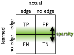
In real applications data is often limited and noisy, and modeling assumptions usually do not hold. So we must assume that there will be errors when learning dependency networks from data. The different types of errors can be visualized in a confusion matrix, as in Figure 1a. Ideally, all edges would be identified as true positives (TP) or true negatives (TN), but this is usually not possible so there will also be some false positives (FP) and false negatives (FN). Using sparse network learning algorithms, such as graphical lasso [7], one can trade off between the two types of errors by adjusting the degree of sparsity of the learned network. This moves the boundary between the learned edges and non-edges shown as the horizontal line highlighted in green in Figure 1a. Assuming the algorithm is able to identify edges with better than random probability, the precision ($\text{TP}/(\text{TP}+\text{FP})$) will increase with sparsity; meanwhile, the recall ($\text{TP}/(\text{TP}+\text{FN})$) will decrease. Figure 1c shows that this is indeed the case. The figure plots the edge recall vs. the edge precision for networks learned from training sets of various sizes. The true network has 1000 nodes and 1000 edges. Each line is generated by changing the sparsity to obtain different edge precision-recall tradeoffs. For denser networks, recall is high, but precision is lower. As networks get sparser, the precision increases but the recall decreases. Thus the degree of sparsity controls the edge precision-recall tradeoff.

(a)

(b)

(c)

(d)

Figure 1: (a) Confusion matrix for learning edges of a single network, (b) Confusion matrix for learning differences between networks A and B, (c) Edge precision-recall graph, (d) Differential precision-recall graph.

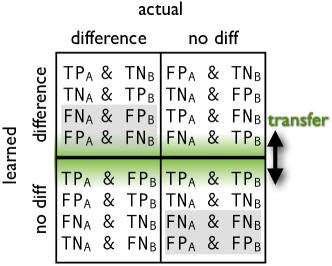
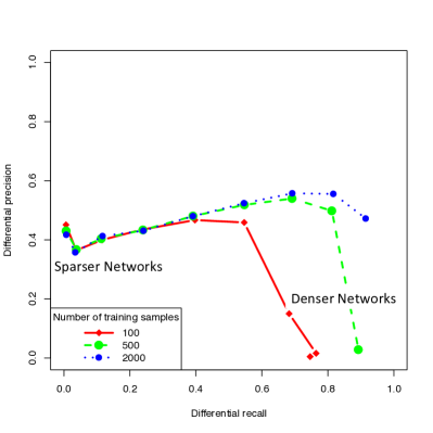
When conducting a differential network analysis (i.e. identifying differences between networks), one would like to control in a similar manner the tradeoff between the differential precision (the percentage of the inferred differences that are actually true) and the differential recall (the percentage of true differences that are recovered). Unfortunately, the traditional approach of learning the networks independently and comparing them provides no mechanism for controlling the differential precision-recall tradeoff. Also, adjusting the sparsity of the learned networks will not help with obtaining the high differential precision required in many applications (e.g. in biological applications, a differential precision above 80% (FDR of 20%) is desirable). Figure 1d plots the differential precision versus the differential recall for pairs of networks learned from training sets of various sizes. The true networks have 1000 nodes and 1000 edges and about 80% of edges in common. Each line is obtained by varying the sparsity of the learned networks. While adjusting the sparsity has some influence on the differential precision and recall, the differential precision never gets above 60%. The reason for this is that the sparsity controls a tradeoff between two types of mistakes: inferring an edge where no edge exists, and missing a true edge (FP and FN in figure 1a). Both types of mistakes will lower the differential precision if the other network does not make the same mistake (see Figure 1b), so trading off between them will not improve the differential precision.

It is important to note that getting more data will not solve this problem. Increasing the training set size four fold from 500 to 2000 instances per task barely improves the differential precision. Also note that the learning algorithm does a very good job at recovering the individual networks (Figure 1c). Thus, short of learning almost perfect networks which is usually impossible in practice, simply improving the performance of the individual network learning algorithms will not be enough to obtain the high differential precision required in many practical applications.

3 Obtaining a Differential Precision-Recall Tradeoff

The differential confusion matrix in Figure 1b provides a clue about how to obtain the desired differential precision-recall tradeoff: the horizontal line can be controlled by imposing an inductive bias towards learning similar networks. A stronger bias for similar networks leads to fewer learned differences, while a weaker bias leads to more learned differences. Assuming that true differences can better overcome this bias, the differential precision will increase with a stronger bias, while the differential recall will probably decrease. Thus the strength of the bias for similar networks is controlling the differential precision-recall tradeoff much in the same way the sparsity bias controls the edge precision-recall tradeoff.

To impose an inductive bias towards learning similar networks, we borrow techniques developed in the transfer learning literature. In transfer learning or multi-task learning, inductive bias towards similar networks is used to obtain more accurate dependency structures when the true networks are similar [3, 4, 5]. The same algorithms can be employed to control the differential precision-recall tradeoff. We emphasize that, even though the learning algorithm is the same, the goal is different. In transfer learning the goal is to improve the accuracy of the individual networks while in this paper the goal is to improve the differential precision and control the differential precision-recall tradeoff. As we shall see, this different goal makes the technique more widely applicable and easier to use. For instance we do not need to assume that the true networks are similar.

In this paper, we use the joint graphical lasso algorithm from [3], which we very briefly describe below. However, other transfer learning algorithms can be used as well. Assuming that the differential analysis is performed over $K$ conditions or populations, the algorithm infers a precision matrix $\widehat{\Theta}_{k}$ for each condition by solving the following joint optimization problem:

$$\arg\max_{\Theta_{k}\succ 0,\forall k}\sum_{k=1}^{K}\left[\log\det\Theta_{k}-\operatorname{tr}(\widehat{\Sigma}_{k}\Theta_{k})\right]-\\ \lambda_{1}\sum_{i\neq j}\left[(1-\lambda_{2})\sum_{k=1}^{K}|\theta_{k,ij}|+\lambda_{2}\left(\sum_{k=1}^{K}\theta_{k,ij}^{2}\right)^{1/2}\right]$$

where $\widehat{\Sigma}_{k}$ is a generalized correlation matrix estimated from the data. If Gaussian covariance is used as a measure of correlation, then a multi-variate Gaussian distribution is fitted to the data of each condition. In this paper we measure correlation using Kendall’s Tau which expands the model class to transelliptical graphical models and leads to increased robustness to outliers and non-Gaussianity without a significant loss in performance [8]. After $\widehat{\Theta}_{k}$ are learned, a dependency network for each domain is obtained by connecting all the variables that have a non-zero entry in $\widehat{\Theta}_{k}$, and differences between domains are obtained by comparing these networks.

The parameter $\lambda_{1}$ controls the sparsity bias for the learned networks, while $\lambda_{2}$ ($0\leq\lambda_{2}\leq 1$) is the similarity bias parameter and controls the strength of the bias towards learning similar networks. When $\lambda_{2}=0$, there is no bias towards similar networks and is equivalent to the traditional method of learning a network for each condition independently. As $\lambda_{2}$ approaches $1$, the bias towards learning similar networks gets stronger, and only differences that are highly supported in the data survive. At $\lambda_{2}=1$ the learned structures will be identical and no differences will be recovered.

4 Experiments with Synthetic Data

We first test the approach using synthetic networks and data. To create a synthetic data set, we generate a network with 1000 Gaussian variables and 1000 undirected edges. Then, the endpoint of each edge is re-wired with some probability to another node, creating a different network with edges in common with the first one. The goal is to correctly identify the differences between the two networks. For each network $k$ we generate a precision matrix $\Theta_{k}$ by independently sampling each entry that corresponds to and edge from a normal distribution, then re-scaling to ensure that $\Theta_{k}$ is positive definite. Training data is then drawn from $\mathcal{N}(0,\Theta_{k}^{-1})$ for each condition $k$. Results are averaged across 5 trials.

(a) Various sample sizes

(b) Various sparsity levels

(c) Various rewiring probabilities

(d) Transfer vs. standard bootstrap

Figure 2: Differential precision-recall curves on synthetic data.

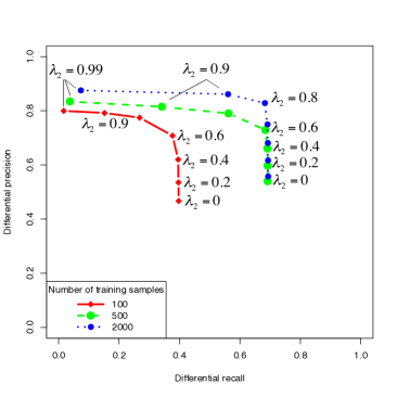
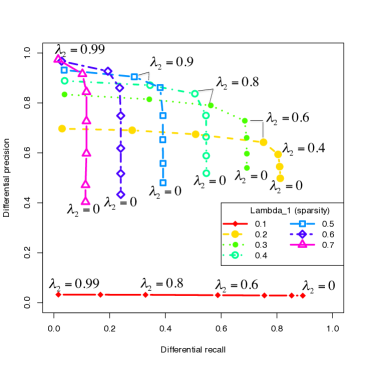
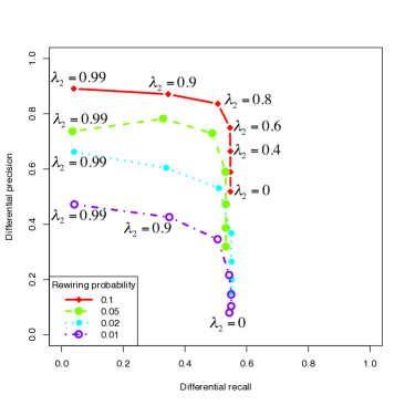
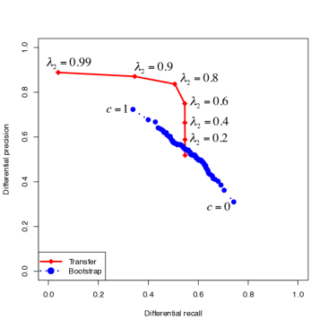
The results of the experiments are depicted in Figure 2 in terms of differential precision-recall curves. In these plots, the differential precision-recall curves are obtained by varying the similarity bias parameter $\lambda_{2}$ between 0 and 1 to obtain different tradeoffs between differential precision and recall. For $\lambda_{2}=0$ we recover the performance of the traditional approach of learning the networks independently and comparing them. This is always the rightmost point of each differential precision-recall curve, with the highest recall but the lowest precision.

Figure 2a shows the differential precision-recall curves for different training set sizes. For each training set size, the sparsity parameter $\lambda_{1}$ is set to the value that yields the highest differential precision in Figure 1d (i.e. the best differential precision obtained by learning the networks independently and comparing them). For all data sizes, increasing the similarity bias (increasing $\lambda_{2}$) improves the differential precision, showing that the proposed technique does indeed enable a more reliable differential analysis. Even with as little data as 100 instances per condition, we are able to obtain a differential precision above 0.8 which would be considered acceptable in many applications. The price to pay is a reduction in the number of differences recovered (reduction in differential recall). Note that in our case there is no a priori “correct” value for the similarity bias parameter. Different values lead to different tradeoffs between the differential precision and recall, and the right operating point depends on the application and even on the analysis stage (similar to ROC analysis in standard classification). In contrast, in the usual use of transfer learning where the goal is to recover the individual networks, there is a “correct” value for this parameter that depends on how similar the true networks are (if the similarity bias is too strong performance will drop due to negative transfer, while if the similarity bias is too weak not enough useful information is transferred between tasks.).

While the tradeoff between precision and recall for learned differences is mainly controlled by the $\lambda_{2}$ parameter, the sparsity parameter, $\lambda_{1}$, also has an effect on the differences learned because it controls which edges are present in each network. Figure 2b shows the differential precision-recall tradeoff for various values of $\lambda_{1}$. Lower values of $\lambda_{1}$ (denser networks) increase the differential recall by identifying differences due to weaker dependencies that do not appear in the sparser graphs. However, the differential precision is lowered because more fake edges are learned in each graph which induce fake differences. At the extreme when the networks are too dense ($\lambda_{1}=0.1$), there are ten times more spurious edges than real ones so the differential precision is low even when the similarity bias is high.

We also vary the rewiring probability when generating the true networks, varying the number of true differences. Figure 2c shows the differential precision-recall graphs for various values of the rewiring probability for $\lambda_{1}=0.4$. As the fraction of true differences decreases (lower rewiring probability), it gets harder to identify them and performance drops. Increasing the similarity bias (increasing $\lambda_{2}$), however, still leads to higher differential precision. These results highlight another fundamental difference with the usual use of transfer learning. In transfer learning the true networks must be similar in order to get any benefit, while in differential analysis there is no such constraint. In fact, in differential analysis performance improves if the true networks are more dissimilar, as opposed to transfer learning where performance gets better with more similar true networks.

Finally, we compare to using bootstrap procedures to identify higher confidence differences. For the bootstrap procedure, we generate a bootstrap sample of the data, train independent graphical models on that data, then compare the learned networks. We repeat this 44400 times. For each edge, $e$, we calculate the bootstrap frequency, $P_{B}(e)$, of it appearing in one network but not the other (i.e. $e$ is a difference). For a given cut-off, $c$, we consider all edges with $P_{B}(e)\geq c$ as inferred differences. We then generate a differential precision-recall graph by varying $c$ from 0 to 1 so that at $c=0$ any difference that appeared in any bootstrap is considered a difference, and at $c=1$ only differences that appear in all 500 bootstraps are considered differences. Figure 2d shows the comparison between the transfer method and the bootstrap method for $\lambda_{1}=0.4$. The transfer method dominates the precision-recall curve compared to bootstrapping, and, importantly, can reach a high precision regime that is unattainable via bootstrapping. Also, the transfer method requires about a factor of 50 less computation than the bootstrapping (the transfer method learns the networks about 10 times, once for each setting of $\lambda_{2}$, while bootstrapping learns the networks 500 times, once for each bootstrap). Moreover, the bootstrapping procedure becomes increasingly computationally expensive as higher levels of differential precision (or recall) are desired. Bootstrapping achieves the highest differential precision when $c=1$ and there are $\sim$100 differences ($\sim$30 of them false) that occur in all 500 bootstraps. Therefore, to push the precision ratio higher than 0.7, we would need to run more bootstraps until these false differences do not appear in at least one of them so they can be filtered out (while hoping that some true differences remain).

5 Real Case Studies

In this section we present three real case studies where domain experts performed differential dependency network analysis in an ovarian cancer study, a pancreatic cancer study, and a neuroimaging study. A quantitative evaluation of the results is difficult in real usage scenarios because there is no ground truth to compare against so true differential precision and recall can not be calculated. In these cases, the usual approach is to estimate the false discovery rate (FDR) through permutation tests. We take the following approach to estimating FDR: first pool the data from all populations (conditions) together, then randomly split the data into synthetic populations with the same number of instances as the original ones. There should not be any difference between the dependency structures of the newly generated synthetic populations, so any difference identified by the algorithm is a false discovery. The splitting procedure is performed multiple times and the average FDR is used as an estimate of the FDR of the algorithm on the original problem. This approach obviously is not perfect and can underestimate the FDR. When tested on synthetic data we found that the true FDR is indeed underestimated.

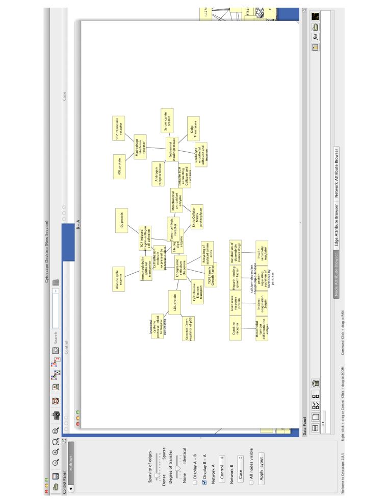
When learning dependency differences from data, we have observed from real users that the best use of multi-network learning is as a part of an exploratory tool that allows interactive exploration of the various tradeoffs controlled by the sparsity and transfer parameters. To this end, we provide the domain experts with a Cytoscape [9] plugin that allows them to interactively explore different settings of $\lambda_{1}$ and $\lambda_{2}$ and quickly identify and visualize the differences in the dependency networks (see Appendix C). For the most part there is no “correct” setting of the parameters as different tradeoffs convey different information about the domain and the right operating point changes depending on the application and even on the analysis stage.

5.1 Oncology Studies

Domain experts applied the technique described in this paper to perform differential dependency network analysis with the goal of identifying and analyzing cancer-induced changes in the dependency structure of plasma proteins. They analyze two cancers: ovarian and pancreatic. The ovarian cancer study uses data from a cohort of 247 patients (114 cases and 133 controls). The pancreatic cancer study uses a cohort of 469 patients (239 cases and 230 controls). Each patient had a blood sample taken prior to the diagnosis, and plasma concentrations of 858 proteins were measured using Somamer technology [10].

(a) Ovarian Cancer

(b) Pancreatic Cancer

Figure 3: Oncology studies. Tradeoff between FDR and number of differences.

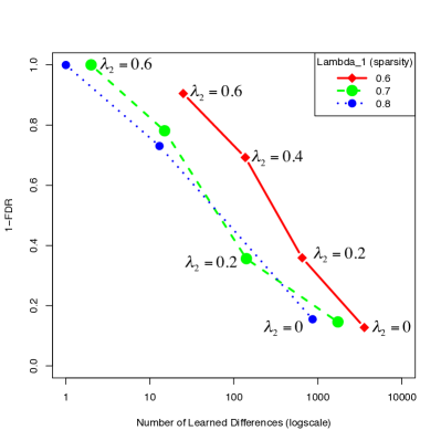
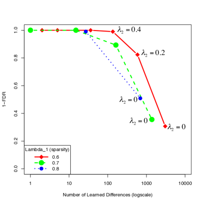
Analogous to the precision recall curves in Figure 2, Figure 3 shows the tradeoff between estimated differential precision (1-FDR) and the number of differences found (in log-scale) for the Ovarian and Pancreatic cancer studies. In both cases, the standard approach of learning the networks independently and comparing them ($\lambda_{2}=0$ at the right end of the curves) discovers between 1000 and 5000 differences, but the majority of them (almost 90% for Ovarian and more than 50% for Pancreatic) are estimated to be false. This level of false discovery renders the results of the differential analysis pretty much useless. However, as the bias for learning similar networks ($\lambda_{2}$) increases, the estimated FDR steadily decreases for all settings of the sparsity parameter, reaching levels below 10% which is very acceptable in biological applications. As in the synthetic data, fewer differences are found, but we have much higher confidence that the remaining differences are real.

Figure 4: Differential dependency network between Case and Control populations in the Ovarian oncology study. Each edge represents a dependency that is present in the cancer population but not in the control population.

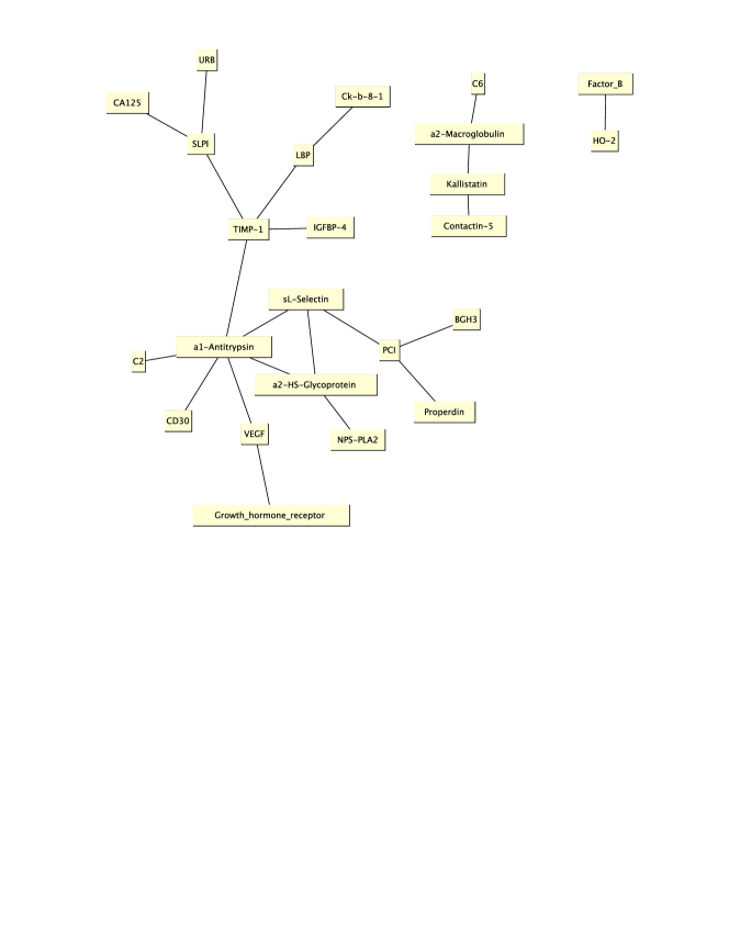
Figure 4 shows the differential dependency network between the cancer and control populations in the Ovarian study for $\lambda_{1}=0.6$ and $\lambda_{2}=0.6$. Every arc in this network represents a dependency that is present in the cancer population but not in the control population. For comparison, we also show the differential dependency network obtained using the standard technique ($\lambda_{1}=0.6$, $\lambda_{2}=0$) in Figure 7 in Appendix A. To ensure that the differential network in figure 4 reveals relevant biological information, we ran a standard enrichment analysis using DAVID [11] on the 24 proteins that appear in the figure, and asked collaborators with extensive expertise in cancer biology to analyze the results. The enrichment analysis shows that the following functional clusters are significantly enriched: endopeptidase inhibitor, inflammatory response, complement and coagulation, and extracellular matrix. This is consistent with what is known about ovarian cancer biology. The body’s reaction to ovarian cancer includes stimulation of both the adaptive (antibodies, cellular immunity) and innate (complement, inflammation) immune systems. In fact, the new “foreign” entity (ovarian cancer) that stimulates these responses also creates a new milieu in which tumor mutations are selected for when they help the cancer evade these immune responses [12]. Ovarian cancers (as well as many other cancers) also tend to induce a hyper-coagulable state, which involve coagulation and complement proteins. Endopeptidases play essential roles in homeostasis and signal transduction. Changes in the extracellular matrix are also key to the process as cancer cells escape the primary tumor and metastasize. A list of proteins associated with each of these processes is given in Appendix A. Many of the proteins in Figure 4 have been associated with cancer in general and with ovarian cancer in particular. For instance CA125 is a well known and clinically used ovarian cancer marker; SLPI has been shown to be over-expressed in gastric, lung and ovarian cancers, accelerating metastasis [13]; VEGF is involved in the growth of blood vessels; IGFBP4 has been associated with a number of cancers, including ovarian [14];

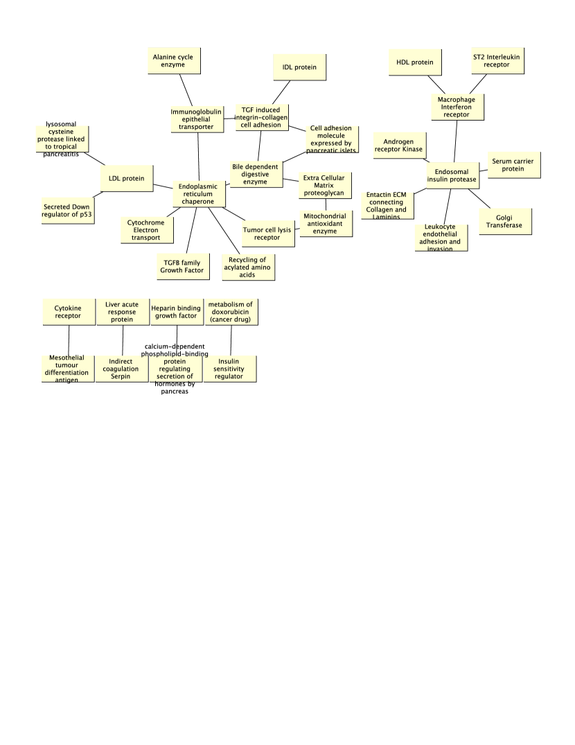
Figure 5 shows the differential dependency network between the cancer and control populations in the pancreatic cancer study for $\lambda_{1}=0.6$ and $\lambda_{2}=0.6$, with the node labels showing functional descriptions in lieu of the protein names. The differential dependency network shows proteins linked with the endocrine pancreas (e.g. endosomal insulin protease, insulin sensitivity regulator, protein regulating secretion of hormones by pancreas) and with the exocrine pancreas (e.g, HDL, LDL, IDL proteins, bile dependent digestive enzyme), as well as proteins associated with cancer and cancer related processes (e.g. tumor cell lysis receptor, mesothelial tumor differentiation antigen, down regulator of p53, endoplasmic reticulum chaperone). An enrichment analysis finds the following processes to be significantly enriched: extracellular matrix, lipid transport and cell adhesion. These processes are relevant to the pancreatic cancer biology. As mentioned above, changes in the extracellular matrix are involved in cancer cells escaping the primary tumor and metastasizing. Related to the extracellular matrix, cell adhesion is also a key process that regulates the migration (spreading) of cancer cells through the body and the destruction of the histological structure in cancerous tissues [15]. The lipid transport is related to the exocrine pancreatic function [16].

Figure 5: Differential dependency network between Case and Control populations in the Pancreatic oncology study. Each edge represents a dependency that is present in the cancer population but not in the control population.

5.2 Accelerated Learning fMRI Study

Functional magnetic resonance imaging (fMRI) measures the activity level in regions of the brain while a subject is in the scanner. The dependency network between regions of interest (ROI) in the brain, is called a functional brain network because it indicates which regions have activity patterns that appear to be exchanging information with each other. A common question is whether these dependencies are different in subjects under different conditions.

Using data from the Accelerated Learning fMRI Study, we want to see how brain regions interact before and after a person learns a new skill [17]. In this study, subjects are asked to identify concealed objects in still images taken from a virtual reality environment. Initially, all subjects are considered Novice (i.e. not significantly better than random at identifying images with concealed objects). fMRI data are collected from these subjects while performing this identification task. Then, subjects are trained until they reach a level of Intermediate competency (midway between chance and perfect). At this point, fMRI data are again collected while performing the identification task. In total, we have data from 12 subjects at the Novice stage and 4 at the Intermediate stage. For each subject, there are 1056 samples of brain activity from 116 regions of interest (ROIs) in the brain. The ROIs are defined by the AAL atlas [18]. The goal is to identify dependencies among the ROIs that are different between the Intermediate and Novice stages. Looking at the networks (rather than the activity levels of individual ROIs) shows us which ROIs are most critical for performing a cognitive task [17].

(a)

(b)

(c)

Figure 6: Accelerated Learning study. (a) Tradeoff between FDR and number of differences (b) Edges in Novice but not in Intermediate, (c) Edges in Intermediate but not in Novice

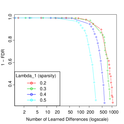
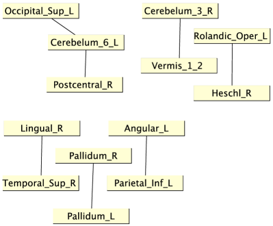
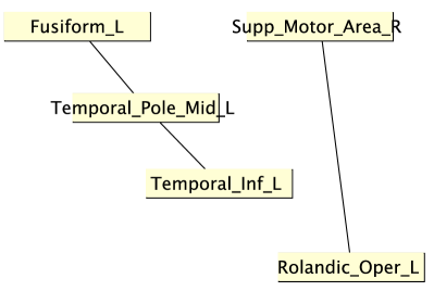
Figure 6a shows the tradeoff between the estimated differential precision (1-FDR) and the number of differences found (in log-scale) for different values of $\lambda_{1}$. As before, $\lambda_{2}$ is varied to obtain each curve. Using the standard approach ($\lambda_{2}=0$, lower right end of the curves), one identifies from 300 to 1000 differences between novice and intermediate functional brain networks, but almost 80% of them are estimated to be false. As the similarity bias increases, the estimated FDR decreases rapidly to levels close to 0 (again, remember that this is an optimistic estimate), so we are much more confident that we are identifying true differences in the functional brain networks.

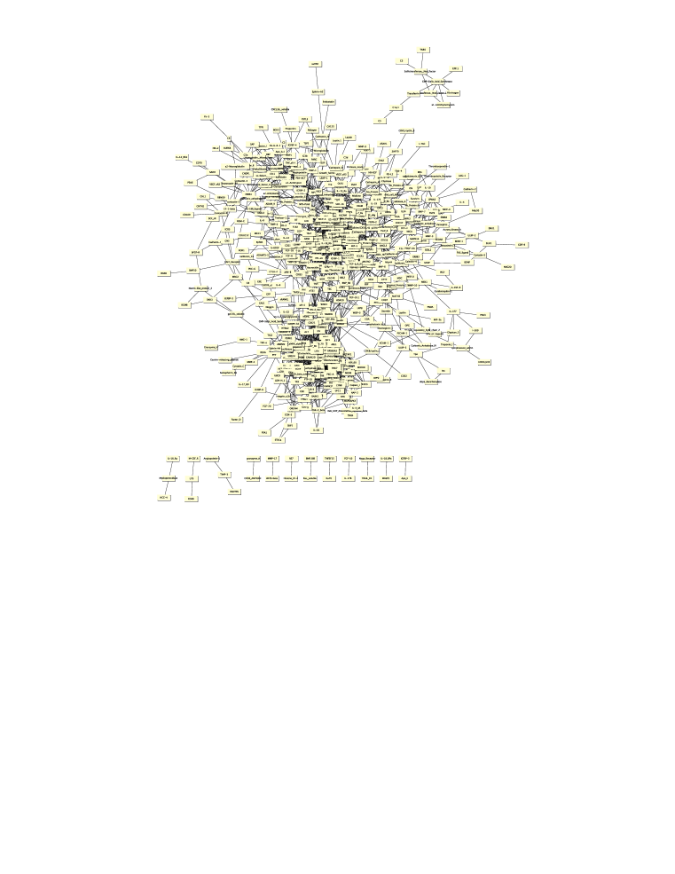
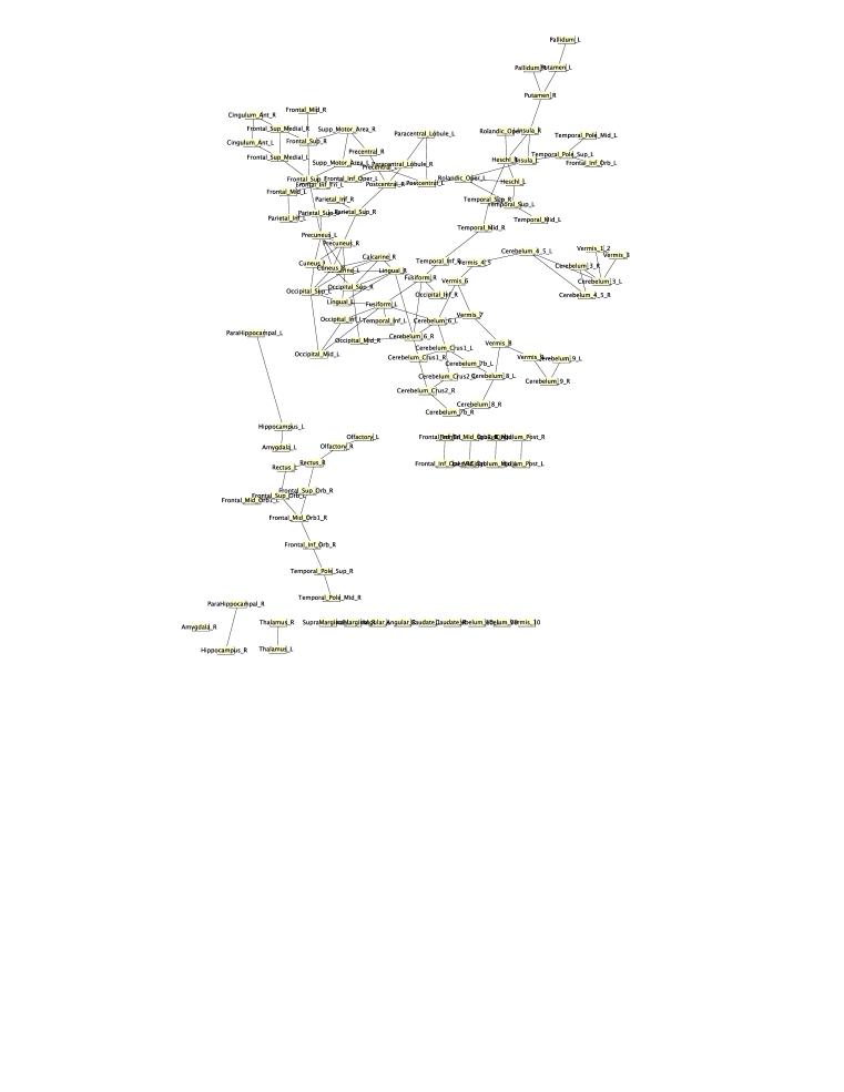
Figures 6b and 6c show the connections that appear in novices but not in intermediates, and vice versa for $\lambda_{1}=0.5$ and $\lambda_{2}=0.2$ (these parameter settings were selected by the domain expert to give just a handful of dependencies of high confidence). Figure 8 in Appendix B also shows the connections present in both novices and intermediates. These results show that for both stages, groups of brain regions are found that share information, which correlate well with sensori-motor pathways found in humans. This includes the occipito-parietal dorsal visual pathway that computes the location of objects, the occipito-temporal ventral pathway that determines the identity of objects, collections of frontal and cingulate regions that help to make decisions about responses, as well as separate cerebellar and middle temporal networks, along with other smaller networks of brain regions [19]. With learning to identify hidden objects in this task, it was found that portions of the ventral pathway increased in strength, suggesting that learning resulted in greater information flow among regions that specialize in visual object identification.

6 Conclusion

Differential analysis of dependency networks of multivariate data allows domain experts to uncover and understand the differences between related populations and the processes that are generating these differences. Such questions arise in many domains including biology, medicine, and neuroscience. We have shown that the traditional approach of learning the dependency networks for each task independently and comparing them is prone to having high false discovery rates. We have discussed the importance of controlling the quality of the inferred differences between dependency networks, and explored a novel use of transfer learning techniques to provide a natural and explicit “knob” that controls the precision-recall tradeoff in differential network analysis. We have shown empirically that this approach achieves higher precision than existing methods, and yields better performance than significantly more expensive bootstrapping procedures. Finally, we have presented three real case studies where domain experts used the proposed techniques to uncover compelling evidence of biological processes involved in cancer and human learning.

While in this paper we have focused on differential network analysis, the idea of using transfer learning techniques to improve differential analysis is quite general. For instance, similar techniques could be used in conjunction with feature selection to answer questions like “are there different cancer biomarkers for men and women?”, or in conjunction with clustering/unsupervised learning to detect significant changes in cluster structures between conditions.

Appendix A Ovarian Cancer Results

Immune response proteins	Inflammatory response proteins	Coagulation and complement proteins	Proteins that are involved in the extracellular matrix	Endopeptidase inhibitor proteins
a2-Macroglobulin	a2-Macroglobulin	a2-Macroglobulin	TIMP1	SLPI
C2	Ck-b-8-1	C2	TIMP1	TIMP1
C6	GHR	C6	URB	a2-Macroglobulin
Ck-b-8-1	LBP	Factor B	a1-Antitrypsin	a2-HS-Glycoprotein
Factor B	a1-Antitrypsin	a1-Antitrypsin	BGH3	a1-Antitrypsin
Properdin	TIMP-1	PCI	VGEF	Kallistatin
GHR	CD30	TIMP-1		PCI
LBP	VEGF	CD30
sL-Selectin	a2-HS-Glycoprotein	VEGF
a1-Antitrypsin
TIMP-1
VEGF
CA-125 may also be involved in these responses.

Table 1: Proteins from the Ovarian cancer differential network that are involved in each of the enriched functional processes.

Figure 7: Differential network for Ovarian cancer obtained using the traditional method of learning the dependency networks independently and compare them ($\lambda_{1}=0.6$, $\lambda_{2}=0$).

Appendix B Accelerated Learning fMRI Results

Figure 8: Network of dependencies shared among Novice and Intermediate stages of the Accelerated Learning study. The network gives valuable re-assurance that the network learning algorithm is identifying true pathways.

Appendix C Interactive Visualization of Differential Dependency Networks

Figure 9: Cytoscape plugin for interactive visualization of the differential networks and exploration of the differential precision-recall tradeoffs.

References

- [1] B. Zhang, H. Li, R.B. Riggins, M. Zhan, J. Xuan, Z. Zhang, E.P. Hoffman, R. Clarke, and Y. Wang. Differential dependency network analysis to identify condition-specific topological changes in biological networks. Bioinformatics, 25(4):526–532, 2009.
- [2] D. Grossman and P. Domingos. Learning Bayesian network classifiers by maximizing conditional likelihood. In Proceedings of the Twenty-First International Conference on Machine Learning, page 46, 2004.
- [3] Patrick Danaher, Pei Wang, and Daniela Witten. The joint graphical lasso for inverse covariance estimation across multiple classes. arXiv stat.ME, 1111(00324v1), November 2011.
- [4] Julien Chiquet, Yves Grandvalet, and Christophe Ambroise. Inferring multiple graphical structures. Statistics and Computing, 21(4):537–553, October 2011.
- [5] J. Guo, E. Levina, G. Michailidis, and J. Zhu. Joint estimation of multiple graphical models. Biometrika, 98(1):1, 2011.
- [6] Karthik Mohan, Mike Chung, Seungyeop Han, Daniela Witten, Su-In Lee, and Maryam Fazel. Structured learning of Gaussian graphical models. In Advances in Neural Information Processing Systems 25, pages 629–637. 2012.
- [7] Nicolai Meinshausen and Peter Bühlmann. High-dimensional graphs and variable selection with the lasso. The Annals of Statistics, 34(3):1436–1462, June 2006.
- [8] Han Liu, Fang Han, and Cun-Hui Zhang. Transelliptical graphical models. In Advances in Neural Information Processing Systems 25, pages 809–817. 2012.
- [9] Paul Shannon, Andrew Markiel, Owen Ozier, Nitin S Baliga, Jonathan T Wang, Daniel Ramage, Nada Amin, Benno Schwikowski, and Trey Ideker. Cytoscape: a software environment for integrated models of biomolecular interaction networks. Genome research, 13(11):2498–2504, 2003.
- [10] Larry Gold, Deborah Ayers, Jennifer Bertino, Christopher Bock, Ashley Bock, Edward N Brody, Jeff Carter, Andrew B Dalby, Bruce E Eaton, Tim Fitzwater, et al. Aptamer-based multiplexed proteomic technology for biomarker discovery. PloS one, 5(12):e15004, 2010.
- [11] Da Wei Huang, Brad T Sherman, and Richard A Lempicki. Systematic and integrative analysis of large gene lists using DAVID bioinformatics resources. Nat. Protocols, 4(1):44–57, 12 2008.
- [12] Xipeng Wang, Ena Wang, John J Kavanagh, and Ralph S Freedman. Ovarian cancer, the coagulation pathway, and inflammation. Journal of Translational Medicine, 3(1):25, 2005.
- [13] Baik-Dong Choi, Soon-Jeong Jeong, Guanlin Wang, Jin-Ju Park, Do-Seon Lim, Byung-Hoon Kim, Yong-Ick Cho, Chang-Seok Kim, Moon-Jin Jeong, et al. Secretory leukocyte protease inhibitor is associated with MMP-2 and MMP-9 to promote migration and invasion in SNU638 gastric cancer cells. International Journal of Molecular Medicine, 28(4):527, 2011.
- [14] Graeme Walker, Kenneth MacLeod, Alistair RW Williams, David A Cameron, John F Smyth, and Simon P Langdon. Insulin-like growth factor binding proteins IGFBP3, IGFBP4, and IGFBP5 predict endocrine responsiveness in patients with ovarian cancer. Clinical Cancer Research, 13(5):1438–1444, 2007.
- [15] Setsuo Hirohashi and Yae Kanai. Cell adhesion system and human cancer morphogenesis. Cancer Science, 94(7):575–581, 2005.
- [16] Angel Lopez-Candales, Matthew S Bosner, Curtis A Spilburg, and Louis G Lange. Cholesterol transport function of pancreatic cholesterol esterase: directed sterol uptake and esterification in enterocytes. Biochemistry, 32(45):12085–12089, 1993.
- [17] Vincent P Clark, Brian A Coffman, Andy R Mayer, Michael P Weisend, Terran D R Lane, Vince D Calhoun, Elaine M Raybourn, Christopher M Garcia, and Eric M Wassermann. TDCS guided using fMRI significantly accelerates learning to identify concealed objects. Neuroimage, 59(1):117–128, Jan 2012.
- [18] N Tzourio-Mazoyer, B Landeau, D Papathanassiou, F Crivello, O Etard, N Delcroix, B Mazoyer, and M Joliot. Automated anatomical labeling of activations in SPM using a macroscopic anatomical parcellation of the MNI MRI single-subject brain. Neuroimage, 15(1):273–289, Jan 2002.
- [19] Mortimer Mishkin, Leslie G Ungerleider, and Kathleen A Macko. Object vision and spatial vision: two cortical pathways. Trends in Neurosciences, 6:414–417, 1983.