Dynamic Service Rate Control for a Single Server Queue with Markov Modulated Arrivals

Abstract

We consider the problem of service rate control of a single server queueing system with a finite-state Markov-modulated Poisson arrival process. We show that the optimal service rate is non-decreasing in the number of customers in the system; higher congestion rates warrant higher service rates. On the contrary, however, we show that the optimal service rate is not necessarily monotone in the current arrival rate. If the modulating process satisfies a stochastic monotonicity property the monotonicity is recovered.

We examine several heuristics and show where heuristics are reasonable substitutes for the optimal control. None of the heuristics perform well in all the regimes. Secondly, we discuss when the Markov-modulated Poisson process with service rate control can act as a heuristic itself to approximate the control of a system with a periodic non-homogeneous Poisson arrival process. Not only is the current model of interest in the control of Internet or mobile networks with bursty traffic, but it is also useful in providing a tractable alternative for the control of service centers with non-stationary arrival rates.

1 Introduction

In this paper, we study a fundamental queueing control problem; managing the service rate of a server in the face of non-stationary arrival rates. We have a queue with an infinite buffer and a single server. Arrivals occur according to a Markov-modulated Poisson process (MMPP), which is to say that the rate of the Poisson process driving the arrivals into the system changes according to an exogenous Markov process. This exogenous Markov process is commonly referred to as the phase modulating process. The service times are assumed to be exponential. We incur a holding cost for each job in the system and there is a cost for running the server at different service rates. Given that the state of the phase modulating process and state of the queue are known, we want to find a policy to adjust the service rate so as to minimize either the expected discounted cost or the long-run average cost rate over an infinite horizon.

Our model is motivated by the power aware transmission policies that are becoming increasingly important over the Internet and in mobile networks. The goal of such policies is to control the power consumption of wireless devices by adjusting the transmission rate in response to the number of packets waiting to be transmitted in the buffer. Due to changes in incoming and outgoing traffic through the device, it is almost always the case that the packet arrivals display non-stationarities, creating periods of bursts followed by near-complete silence. Our use of an MMPP to model arrivals is intended to capture such periods of bursts and silence. An alternative model to capture the non-stationary nature of arrivals is the non-homogenous Poisson process (NHPP), but for the wireless applications we have in mind, MMPP appears to be a more suitable model of non-stationarity since these applications involve arrival rate changes occurring at random points in time, whereas an NHPP models arrival rates as a fixed function of time. Furthermore, when computing the optimal policy under an NHPP, one needs to keep track of time together with the queue length, resulting in an uncountable state space. This issue is not present when dealing with an MMPP.

Controlling queues when arrivals have varying rates poses interesting challenges. When controlling such queues, the policy in use not only needs to consider the current arrival rate, but it also needs to anticipate the arrival rate in the near future and adjust decisions accordingly. For example, if the current arrival rate is relatively low, but arrivals are expected to be more frequent in the near future, then the control policy may choose to proactively speed up the service rate to empty the system (as much as possible) before the higher arrival rate strikes. Similarly, if the current arrival rate is high and the current system load is high, the control policy may slow down the service rate in anticipation of lower arrival rates in the near future. The extent to which changes in arrival rates can be foreseen or anticipated depends on how the non-stationarity is modeled, but policies that explicitly address the non-stationarity in arrival rate are naturally expected to make better decisions than those that do not. Furthermore, the need to model arrival non-stationarities is becoming increasingly important as non-stationary queues find more use in telecommunications applications to study congestion problems on the Internet and mobile networks.

We provide a characterization of how the optimal policy depends on the queue length and the arrival rate. Throughout, we assume that the arrival intensities change according to a general continuous time Markov chain (CTMC) defined on the state space $\{1,2,\dots,L\}$ and the arrival rates of the MMPP are ordered such that $\lambda_{1}\leq\lambda_{2}\leq\dots\leq\lambda_{L}$. In this context, the first interesting question is whether the optimal service rate is monotone in the queue length, for a fixed state of the phase modulating process. We answer this question, not too surprisingly, in the affirmative, indicating that the optimal service rate is higher as we have more jobs in the buffer, all else being equal. The second interesting question is whether the optimal service rate is monotone in the state of the phase modulating process, for a fixed queue length. Perhaps surprisingly, the answer to this question is not necessarily affirmative, indicating that the optimal service rate is not necessarily higher as the arrival rate becomes larger, all else being equal. This observation builds the intuition that the optimal policy should anticipate the arrival rate in near future. For example, even if the current arrival rate is higher, the optimal policy may choose not to serve the jobs faster because the arrival rate is expected to slow down soon after the higher arrival rate strikes. Thus, although it may be surprising to see that the optimal service rate is not necessarily monotone in the state of the phase modulating process, this non-monotonicity embodies the intuitive expectation that the optimal policy may start using faster service rates even before higher arrival rates strike or may start using slower service rates even before arrival rates slow down. Motivated by this observation, a natural question is when we can expect the optimal policy to actually be monotone in the state of the phase modulating process so that the behavior that we just mentioned is not prevalent. We give sufficient conditions under which the optimal service rate is indeed monotone in the state of the phase modulating process. These conditions are simple to check and they only depend on the structure of the CTMC driving the phase process. These structural results are not only important in providing insights but are also useful in deriving efficient approximation methods. When the phase process for the MMPP has a large number of states, computing an optimal policy using value or policy iteration may still be a difficult task. In these situations, the structural properties of the value function can be used to develop approximate dynamic programming methods and obtain approximate results efficiently (see for example Powell[21]).

We include a numerical study with two goals in mind. First, we examine when it is important to explicitly capture the non-stationary behavior of an arrival process via MMPP as opposed to using some natural heuristic like assuming the system has stationary arrivals. To implement the optimal policy, a decision maker needs to look at both the state of the queue and the state of the phase process of the MMPP while a heuristic control mechanism based only on the queue length or some fixed service rate may be easier to implement. Thus, a comparison between the two helps in determining the value of a more complex control mechanism. Second, since we mentioned the alternative of using an NHPP to capture the non-stationarity in the arrivals, we explore the possibility of using a “suitable” MMPP to approximate the control policy for a system with an NHPP with a periodic rate function. We find that our preliminary results are encouraging. This is a significant diversion from previous studies since the focus here is on computing an optimal control and not solely on evaluating performance measures.

Most of the research related to Markov-modulated queueing systems deals with performance characteristics for systems without control. Excellent overviews of this line of work can be found in the survey paper by Prabhu [22] or more recently in Gupta et al. [13]. A hierarchical scheme based on MMPP was proposed by Muscariello et al. [20] to model the data generated by Internet users. Heffess et al. [14] used MMPP to approximate a statistical multiplexer whose inputs consist of superposition of packetized voice sources and data. A two state MMPP model was proposed by Shah-Heydari [24] to model the so-called aggregate asynchronous transfer mode traffic. For more general scenarios, Frost [10] proposed a scheme to approximate a simple NHPP using an MMPP by suitably quantizing the rate function of the NHPP into a finite number of rates. Each rate corresponds to a state in the Markov modulating process and the parameters of the MMPP model can be estimated using empirical data.

There is also a rich body of literature on the subject of monotone optimal policies for the control of a single server queue in a setting similar to the one considered here but with stationary arrivals. See, for example, the classical work of Crabill [6], Lippman [18] and Stidham and Weber [25]. In the context of telecommunications systems, the existing literature addresses a more closely related problem of service rate control of queues when the job service requirements are influenced by an exogenous stochastic process. Such models arise frequently in point-to-point wireless data transmission where the induced transmission rates are affected by the time varying properties of the transmission medium. Berry [3] considers a very general model for this problem under a discrete-time Markovian setting. In this work, packet arrivals follow a batch Markov process and the state of the transmission channel varies according to a secondary discrete-time Markov chain. The data buffer and transmitter are modeled using a single server queue with finite capacity. The goal of the transmitter is to minimize the average cost rate or power consumption over an infinite time horizon subject to a constraint on packet delay. Another case with a constraint on the probability of buffer overflow is also discussed in this work. The author proves several results related to the monotonicity of the optimal policy. Motivated by mobile networks, Ata and Zachariadis [2] address the problem of finding optimal service rates for multiple users that are being served by a central controller. Data gets transmitted through a time varying channel that is being modulated by a two-state continuous time Markov chain. Packet data for each user arrives based on a Poisson process and gets stored in a finite capacity queue before getting transmitted. The objective is to maximize some measure of overall quality of service subject to a constraint on the long-run average power consumption. The authors show that the optimal service rates for each user depend only on its own queue length and the state of the transmission channel. They also present a method to explicitly characterize the optimal policy for each user. To the best of our knowledge, none of the aforementioned work considers the case of a multi-state Markov-modulated arrival process with service rate control as is discussed in this paper.

We have organized this paper as follows. In Section 2 we give a detailed description of the model and the associated assumptions, and formulate the problem as a Markov decision process. In the average cost case we provide stability conditions that guarantee convergence of the discounted cost value function to the relative value function. In Section 3 we give structural results related to the optimal policy in each case. In Section 4, we present a detailed numerical study comparing the performance of the optimal policy with heuristic policies and present an exploratory study related to the computation of a heuristic policy for non-homogeneous Poisson arrivals using the optimal policy for a MMPP/M/1 queue. We conclude the paper in Section 5.

2 Model Formulation

We consider a single server queue with infinite buffer capacity and job arrivals that follow an MMPP. Each arriving job has an exponentially distributed service requirement with mean 1. The phase transition process for arrivals is an ergodic, finite state continuous time Markov chain with generator matrix $Q$. Let the state space for this process be denoted by $\mathcal{S}:=\{1,2,\dots,L\}$. When the phase transition process is in phase $s\in\mathcal{S}$, jobs arrive to the queue according to a Poisson process with rate $\lambda_{s}$. Without loss of generality we assume that the states are ordered such that $\lambda_{1}\leq\lambda_{2}\leq\dots\leq\lambda_{L}$. Let the number of jobs in the system (buffer state) be denoted by $n\in\mathbb{Z}^{+}$, where $\mathbb{Z}^{+}$ is the set of non-negative integers. The service rate can be changed at the times of arrivals, departures or phase transitions. Together, the union of these event times and (in a moment) the added dummy transitions due to uniformization comprise the set of decision epochs. Based on the queue length, $n$, and the state of the arrival process, $s$, the controller selects a service rate $\mu_{n,s}$ from the compact set $\mathbb{A}=[0,\bar{u}]$, $\bar{u}<\infty$. When a service rate $\mu\in\mathbb{A}$ is chosen, the system incurs a cost at the rate of $c(\mu)$ per unit time. The cost rate function, $c(\cdot)$, is defined on $\mathbb{A}$ and is assumed to be strictly convex, continuously differentiable, strictly increasing and (without loss of generality) such that $c(0)=0$. Furthermore, a holding or congestion cost is incurred at rate $h(n)$ per unit time when the buffer state is $n$. The holding cost function $h(n)$ is assumed to be convex, non-decreasing in $n$ and such that $h(0)=0$ and $\lim_{n\rightarrow\infty}h(n)=\infty$. In the average-cost case we assume $h(\cdot)$ to be a non-decreasing and convex with polynomial rate of growth ($h(n)\leq Cn^{p}$ for some $C\geq 0,p\in\mathbb{Z}^{+}$) and again such that $h(0)=0$ and $\lim_{n\rightarrow\infty}h(n)=\infty$. The assumption about polynomial growth rate of the holding cost function for the average cost case is required for proving the existence of a policy that incurs costs at a finite rate.

Let $\Pi$ be the set of non-anticipating policies. A stationary control policy, $\pi\in\Pi$, is defined as $\pi=\{\mu(n,s)\mid n\in\mathbb{N},s\in\mathcal{S}\}$, where $\mu(n,s)$ is the service rate to be selected when the state of the system is $(n,s)$. The controller remains idle when the queue is empty i.e, for any policy, $\mu(0,s)\equiv 0$. Thus, given a policy $\pi$, the overall process, $X(t)$, evolves as a two dimensional continuous time Markov chain on the state space $\mathbb{X}=\{(n,s)\mid n\in\mathbb{Z}^{+},s\in\mathcal{S}\}$. Our objective is to find a control policy that minimizes the discounted expected cost or average expected cost per unit time over an infinite time horizon.

2.1 The Discounted Expected Cost Formulation

For $x=(n,s)$ and service rate $\mu\in\mathbb{A}$, let

$$f(x,\mu):=c(\mu)+h(n).$$

Let $\{(X^{\pi}(t),D^{\pi}(t)),t\geq 0\}$ be the stochastic process representing the evolution of states and decisions under an admissible policy $\pi$. Given the initial state $x$ and discount factor $\alpha>0$, the $\alpha-$discounted expected cost until time $t$ under policy $\pi$ is given by

$$v_{t,\alpha}^{\pi}(x) :=\operatorname{\mathbb{E}}_{x}^{\pi}\left[\int_{0}^{t}e^{-\alpha u}f(X(u),D(u))du\right],$$ (2.1)

where $\operatorname{\mathbb{E}}_{x}[\cdot]:=\operatorname{\mathbb{E}}[\cdot|X(0)=x]$. The total discounted expected cost of a policy $\pi$ given that the initial state of the system is $x$, is

$$v^{\pi}_{\alpha}(x) :=\lim_{t\to\infty}v^{\pi}_{t,\alpha}(x).$$

The optimal total discounted expected cost is

$$v_{\alpha}^{\ast}(x) :=\inf_{\pi\in\Pi}v_{\alpha}^{\pi}(x).$$

A policy, $\pi^{\ast}$, is total discounted expected cost optimal if $v_{\alpha}^{\pi^{\ast}}(x)=v_{\alpha}^{\ast}(x)$ for all $x\in\mathbb{X}$.

We apply uniformization in the spirit of Lippman [18] and consider the discrete time equivalent of the continuous time Markov chain described above. The uniformization rate is chosen to be $\nu:=\lambda_{L}+\bar{\eta}+\bar{u}$, where $\bar{\eta}\geq\max\{-Q_{ss}\mid s\in\mathcal{S}\}$ is any finite rate larger than the maximum of the holding time parameters for the phase transition process.

Let $v_{\alpha,k}(n,s)$ be the minimum total $\alpha$-discounted expected cost that can be obtained during the last $k$ transitions when starting from state $(n,s)$. Using standard arguments of Markov decision theory [4], the discrete-time finite horizon optimality equations (FHOE) for the system can be written (for each $s\in\mathcal{S}$):

$$v_{\alpha,k+1}(0,s) =\frac{1}{\alpha+\nu}\Big{[}h(0)+\lambda_{s}v_{\alpha,k}(1,s)$$

$$\quad+\sum_{s^{\prime}=1}^{L}Q_{ss^{\prime}}v_{\alpha,k}(0,s^{\prime})+(\nu-\lambda_{s})v_{\alpha,k}(0,s)\Big{]}$$ (2.2a)

$$v_{\alpha,k+1}(n,s) =\frac{1}{\alpha+\nu}\min_{\mu\in\mathbb{A}}\bigg{\{}c(\mu)+h(n)+\mu v_{\alpha,k}(n-1,s)+\lambda_{s}v_{\alpha,k}(n+1,s)$$

$$\quad{}+\sum_{s^{\prime}=1}^{L}Q_{ss^{\prime}}v_{\alpha,k}(n,s^{\prime})+\left(\nu-\lambda_{s}-\mu\right)v_{\alpha,k}(n,s)\bigg{\}}\quad\text{ for }n\geq 1,$$ (2.2b)

where $v_{\alpha,0}$ is assumed to be zero for each state. Note that the cost function has compact level sets. That is, $\{((n,s),\mu)|f((n,s),\mu)\leq\beta\}$ is compact for all $\beta\in\mathbb{R}$. Since the state space is discrete, we may apply Proposition 3.1 of [9] to get $v_{\alpha,k}\uparrow v_{\alpha}$. Moreover, $v_{\alpha}$ satisfies (2.2) with $v_{\alpha}$ replacing $v_{\alpha,k}$ on the right hand side and $v_{\alpha,k+1}$ on the left hand side. The resulting set of equations are called the discounted cost optimality equations (DCOE) and are stated next for later reference (for each $s\in\mathcal{S}$).

$$v_{\alpha}(0,s) =\frac{1}{\alpha+\nu}\left[h(0)+\lambda_{s}v_{\alpha}(1,s)+\sum_{s^{\prime}=1}^{L}Q_{ss^{\prime}}v_{\alpha}(0,s^{\prime})+(\nu-\lambda_{s})v_{\alpha}(0,s)\right]$$ (2.3a)

$$v_{\alpha}(n,s) =\frac{1}{\alpha+\nu}\min_{\mu\in\mathbb{A}}\bigg{\{}c(\mu)+h(n)+\mu v_{\alpha}(n-1,s)+\lambda_{s}v_{\alpha}(n+1,s)$$

$$\quad{}+\sum_{s^{\prime}=1}^{L}Q_{ss^{\prime}}v_{\alpha}(n,s^{\prime})+\left(\nu-\lambda_{s}-\mu\right)v_{\alpha}(n,s)\bigg{\}}\text{ for }n\geq 1.$$ (2.3b)

2.2 The Long-Run Average Cost Formulation

In this section we provide conditions under which an average cost optimal policy exists and may be computed as a limit of discounted cost optimal policies. The long-run average cost or gain of a policy $\pi$ given that the initial state of the system is $x$, is

$$g^{\pi}(x) :=\limsup_{t\to\infty}v_{t,0}^{\pi}(x)/t,$$

where $v_{t,0}$ is as defined in (2.1). The optimal expected average cost $g^{\ast}(x)$ is

$$g^{\ast}(x) :=\inf_{\pi\in\Pi}g^{\pi}(x),$$

and $\pi^{\ast}$ is an average cost optimal policy if $g^{\pi}(x)=g^{\ast}(x)$ for all $x\in\mathbb{X}$. After uniformization the average cost optimality inequalities (ACOI) (cf. [23]) are,

$$w(n,s)\geq \frac{1}{\nu}\min_{\mu\in\mathbb{A}}\bigg{[}-g+c(\mu)+h(n)+\lambda_{s}w(n+1,s)+\mu w((n-1)^{+},s)$$

$$+\sum_{s^{\prime}=1}^{L}Q_{ss^{\prime}}w(n,s^{\prime})+(\nu-\lambda_{s}-\mu)w(n,s)\bigg{]}\text{ for }n\geq 0,s\in\mathcal{S}.$$ (2.4)

When the solution, $(w,g)$ to the ACOI exists, $w$ is called a relative value function and $g^{\ast}(x)=g$ is the optimal long-run expected average cost for any initial state $x$.

A solution to the ACOI (2.2) exists under a necessary and sufficient stability condition which is provided in (2.5) below. This condition requires that the maximum available service rate is higher than the long-run average arrival rate and coincides with the one derived by Yechiali [26] for the stability of queue with Markov-modulated arrivals. However, since Yechiali used the balance equations to show the existence of a steady state distribution there is no guarantee of finite long-run average cost. This is required for the MDP formulation provided. Since the phase transition process is assumed to be ergodic, it has unique stationary probabilities denoted by, $\{p_{1},p_{2},\dots,p_{L}\}$.

Proposition 2.1.

There exists a stationary policy ,$\pi$, under which the system is stable (steady state distribution exists) if and only if the maximum available service rate satisfies the following condition

$$\bar{u}>\sum_{s=1}^{L}p_{s}\lambda_{s}.$$ (2.5)

Furthermore, the long-run average cost under this policy, $g^{\pi}(x)$, is finite and independent of the initial state $x$.

Proof.

See Appendix.

In the next proposition, we present results related to the existence of an optimal average-cost policy.

Proposition 2.2.

The following hold

1. For $\alpha>0$, $v_{\alpha}(x)$ satisfies the DCOE (2.3). Moreover, any stationary policy $\pi_{\alpha}$ that minimizes the right side of the DCOE (2.3) is $\alpha$-discounted expected cost optimal.

2. If the stability condition (2.5) holds, we have,

   1. There exists a stationary long-run average expected cost optimal policy $\pi^{\ast}=\{\mu^{\ast}(n,s)\mid n\geq 1,s\in\{1,2,\dots,L\}\}$ that is a limit of a sequence of discounted expected cost optimal policies $\{\pi_{\alpha_{k}},k\geq 1\}$. That is, $\mu^{\ast}(n,s)=\lim_{k\rightarrow\infty}\mu_{\alpha_{k}}(n,s)$, where $\alpha_{k}\downarrow 0$.

   2. The long-run average expected cost of policy $\pi^{\ast}$ is $g^{\ast}=\lim_{\alpha\downarrow 0}\alpha v_{\alpha}(x)$ for every $x\in\mathbb{X}$. Moreover, there exists a subsequence $\alpha_{k}\downarrow 0$ such that $\lim_{k\to\infty}w_{\alpha_{k}}(x):=v_{\alpha_{k}}(x)-v_{\alpha_{k}}(\mathbf{0})=w(x)$ for a distinguished state $\mathbf{0}$ such that $(w,g^{*})$ satisfy the ACOI (2.2).

Proof.

See Appendix.

3 Structural Properties of Optimal Policies

In this section we derive structural results for optimal policies for both the discounted cost and the average cost criterion. In a manner similar to [11], we use following definitions to simplify the optimality equations,

$$y_{\alpha}(0,s) =0\text{ for }s=1,2,\dots,L,$$ (3.1)

$$y_{\alpha}(n,s) =v_{\alpha}(n,s)-v_{\alpha}(n-1,s)\text{ for }n\in\mathbb{N},s\in\mathcal{S},$$

$$\phi(y) =\max_{\mu\in\mathbb{A}}\{\mu y-c(\mu)\},\text{ and }$$

$$\psi(y) =\arg\max_{\mu\in\mathbb{A}}\{\mu y-c(\mu)\},$$

where the argmax is a singleton by the assumptions on $c$ (cf. Section 4.3 of [1]). The definitions above yield the following simplified form of the DCOE (2.3):

$$v_{\alpha}(n,s) =\frac{1}{\alpha+\nu}\bigg{[}h(n)-\phi(y_{\alpha}(n,s))+\lambda_{s}v_{\alpha}(n+1,s)+\sum_{s^{\prime}=1}^{L}Q_{ss^{\prime}}v_{\alpha}(n,s^{\prime})$$

$$\quad{}+(\nu-\lambda_{s})v_{\alpha}(n,s)\bigg{]}\text{ for }n\in\mathbb{Z}^{+},s\in\mathcal{S}.$$ (3.2)

In order to derive structural results for an optimal discounted expected cost policy, we make use of several important properties of functions $\phi(y)=\max_{x\in\mathbb{A}}\{yx-c(x)\}$ and its associated maximizers $\psi(y)=\arg\max_{x\in\mathbb{A}}\{yx-c(x)\}$ that were introduced in the DCOE (2.3). Recall that the conjugate of $c(\cdot)$, $\phi(\cdot)$, is convex (cf. [5]). Moreover, $\psi(y)$ is continuous, non-decreasing and equals $\phi^{\prime}(y)$ wherever the derivative exists. As described in [1], since $(c^{\prime})^{-1}(\cdot)$ is well-defined, continuous and strictly increasing we have the following characterization of the function $\psi(\cdot)$

$$\psi(y) =\begin{cases}0&\text{ if }y\leq c^{\prime}(0),\\ (c^{\prime})^{-1}(y)&\text{ if }c^{\prime}(0)<y<c^{\prime}(\bar{u}),\\ \bar{u}&\text{ if }y>c^{\prime}(\bar{u}).\end{cases}$$ (3.3)

It may also be established (see [11]) that $\phi(\cdot)$ is continuous and non-decreasing with the following characterization

$$\phi(y) =\begin{cases}0&\text{ if }y<0,\\ \int_{0}^{y}\psi(x)dx&\text{ if }y\geq 0.\\ \end{cases}$$ (3.4)

3.1 Monotone In The Number of Customers

We show the intuitive result that there exists an optimal policy that is monotone in $n$. We note that the structural part of the result could also be proven via the event-based dynamic programming framework of Koole [17]. We provide what we believe is an equally simple proof here for completeness.

Proposition 3.1.

The following hold

1. For each $s\in\mathcal{S}$, the optimal discounted expected cost value function, $v_{\alpha}(n,s)$, satisfies the DCOE (2.3) and is a non-decreasing, convex function of $n$.

2. There exists a discounted expected cost optimal policy $\{\mu_{\alpha}(n,s),n\geq 1,s\in\mathcal{S}\}$ that is non-decreasing in $n$ for each $s\in\mathcal{S}$.

3. Under the assumptions that the holding cost is non-decreasing and convex with polynomial rate of growth and (2.5) hold, there exists a long-run average optimal policy, $\{\mu(n,s),n\geq 1,s\in\mathcal{S}\}$ that is non-decreasing in $n$ for each $s\in\mathcal{S}$.

Proof.

We use induction and the FHOE (2.2) to prove the first result. The result holds trivially for $k=0$. For the inductive step, suppose $v_{\alpha,k}(\cdot,s)$ is non-decreasing and convex on $\mathbb{Z}^{+}$ for each $s\in\mathcal{S}$. Let $u_{n}=\mu_{\alpha,k}(n,s)$ be the optimal service rate for the $(k+1)$-stage problem when the state is $(n,s)$. Suppose we use the potentially sub-optimal decision $u_{n}$ when the state is $(n-1,s)$. The FHOE (2.2) yield,

$$v_{\alpha,k+1}(n-1,s) \leq\frac{1}{\alpha+\nu}\bigg{[}c(u_{n})+h(n-1)+u_{n}v_{\alpha,k}((n-2)^{+},s)+\lambda_{s}v_{\alpha,k}(n,s)$$

$$\quad+\sum_{s^{\prime}=1}^{L}Q_{ss^{\prime}}v_{\alpha,k}(n-1,s^{\prime})+\left(\nu-\lambda_{s}-u_{n}\right)v_{\alpha,k}(n-1,s)\bigg{]},$$

$$\leq\frac{1}{\alpha+\nu}\bigg{[}c(u_{n})+h(n)+u_{n}v_{\alpha,k}(n-1,s)+\lambda_{s}v_{\alpha,k}(n+1,s)$$

$$\quad+\sum_{s^{\prime}\neq s}Q_{ss^{\prime}}v_{\alpha,k}(n,s^{\prime})+\left(\nu+Q_{ss}-\lambda_{s}-u_{n}\right)v_{\alpha,k}(n,s)\bigg{]}$$

$$=v_{\alpha,k+1}(n,s),$$

where the second inequality follows from the induction hypothesis. Thus, $v_{\alpha,k}$ is non-decreasing for all $k$.

To show convexity note that by the inductive hypothesis, $y_{\alpha,k}(n+1,s)=v_{\alpha,k}(n+1,s)-v_{\alpha,k}(n,s)$ is a non-decreasing function of $n$ for each $s\in\mathcal{S}$. Let $u_{n+1}=\mu_{\alpha,k}(n+1,s)$ be the optimal rate for the $(k+1)$-stage problem when the state is $(n+1,s)$ and $u_{n-1}=\mu_{\alpha,k}(n-1,s)$ be the optimal rate when the state is $(n-1,s)$. The DCOE (2.3) imply (for $n\geq 1$)

$$(\alpha+\nu)y_{\alpha,k+1}(n+1,s) \geq h(n+1)-h(n)-u_{n+1}(y_{\alpha,k}(n+1,s)-y_{\alpha,k}(n,s))$$

$$\quad+\lambda_{s}y_{\alpha,k}(n+2,s)+\sum_{s^{\prime}=1}^{L}Q_{s,s^{\prime}}y_{\alpha,k}(n+1,s^{\prime}).$$

Similarly for $y_{\alpha,k}(n,s)=v_{\alpha,k}(n,s)-v_{\alpha,k}(n-1,s)$,

$$(\alpha+\nu)y_{\alpha,k+1}(n,s) \leq h(n)-h(n-1)+(\nu-\lambda_{s})y_{\alpha,k}(n,s)$$

$$\quad-u_{n-1}(y_{\alpha,k}(n,s)-y_{\alpha,k}(n-1,s))+\lambda_{s}y_{\alpha,k}(n+1,s)$$

$$\quad+\sum_{s^{\prime}=1}^{L}Q_{s,s^{\prime}}y_{\alpha,k}(n,s^{\prime}).$$

Using the definitions of $\nu=\lambda_{L}+\bar{\eta}+\bar{u}$ and $\bar{\textbf{Q}}=\bar{\eta}\textbf{I}+\textbf{Q}$ we have,

$$(\alpha+\nu)(y_{\alpha,k+1}(n+1,s)-y_{\alpha,k+1}(n,s)) \geq h(n+1)-2h(n)+h(n-1)$$

$$\quad+(\lambda_{L}+\bar{u}-\lambda_{s}-u_{n+1})\left(y_{\alpha,k}(n+1,s)-y_{\alpha,k}(n,s)\right)$$

$$\quad+u_{n-1}(y_{\alpha,k}(n,s)-y_{\alpha,k}(n-1,s))$$

$$\quad+\lambda_{s}\left(y_{\alpha,k}(n+2,s)-y_{\alpha,k}(n+1,s)\right)$$

$$\quad+\sum_{s^{\prime}=1}^{L}\bar{Q}_{s,s^{\prime}}\left(y_{\alpha,k}(n+1,s^{\prime})-y_{\alpha,k}(n,s^{\prime})\right)$$

$$\geq 0.$$

The second inequality follows as $h(n)$ is convex, the coefficients of $y_{\alpha,k}$ terms are non-negative and the inductive hypothesis. So $y_{\alpha,k}(\cdot,s)$ is non-decreasing on $\mathbb{Z}^{+}$ for all $s\in\mathcal{S}$ as required. Taking limits as $k\to\infty$ yields that $v_{\alpha}$ is non-decreasing and convex; the first result is proven.

Since the function $\psi(\cdot)$ is non-decreasing and $\mu_{\alpha}(n,s)=\psi(y_{\alpha}(n,s))$, we conclude that there exists an optimal policy for the discounted cost problem that is monotonically nondecreasing in the queue length for each $s\in\mathcal{S}$. This is the second result.

For the third result, consider a subsequence of discount factors $\{\alpha_{i},i\geq 0\}$ such that $\alpha_{i}\to 0$ and corresponding discounted cost optimal policies $\mu_{\alpha_{i}}(\cdot,\cdot)$ that converge to an average cost optimal policy $\mu(\cdot,\cdot)$ (see Proposition 2.2). The previous result implies that for each fixed $s\in\mathcal{S}$, $\mu_{\alpha_{i}}(n,s)\leq\mu_{\alpha_{i}}(n+1,s)$. Thus, the same inequality holds for $\mu(\cdot,\cdot)$.  

We remark that we have explicitly used the fact that argmax in $\psi$ is a singleton (which follows from the strict convexity assumption on $c(\cdot)$). When the convexity is not assumed to be strict, the results still hold, but we need to take care to define $\psi$ as the minimal element of the argmax and consider a subsequence of discount factors such that $w_{\alpha_{i}}(x)=v_{\alpha_{i}}(x)-v_{\alpha_{i}}(\mathbf{0})\to w(x)$. Since $v_{\alpha_{i}}(n,s)$ is non-decreasing in $n$, so is $w$ and proof in the average cost case follows in the same way as the discounted cost case except that we use the ACOI instead of the DCOE.

3.2 Monotone in the phase process

Since the states of the phase transition process are ordered such that $\lambda_{1}\leq\lambda_{2}\leq\dots\leq\lambda_{L}$, one might conjecture that the optimal policy is non-decreasing in the phase state, $s$, for each congestion level, $n$. However, we present two examples to show that depending on the transition structure of the phase process, this property may not hold. In both examples, we use value iteration with $\alpha=0.05$ to compute the optimal policy numerically. We consider an exponential cost rate function, $c(\mu)=e^{\mu}-1$, and a linear holding cost function, $h(n)=n$. The set of permissible service rates is $\mathbb{A}=[0,5]$.

(a) Birth and Death

(b) Cyclic

Figure 1: Transition structure of Phase process for Examples 3.1 and 3.2.

Example 3.1.

In this example, the phase process is a birth and death process on the states $\{1,2,3\}$. See Figure 1(a). The infinitesimal generator for the phase process is given by

$$\mathbf{Q}=\left[\begin{matrix}-1&1&0\\ 1&-2&1\\ 0&1&-1\end{matrix}\right],$$

and arrival rates are $\lambda_{1}=0.5,\lambda_{2}=1$ and $\lambda_{3}=1.25$.

Figure 2: Structure of Optimal Policy for Example 3.1

Figure 3: Structure of Optimal Policy for Example 3.2

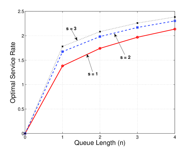
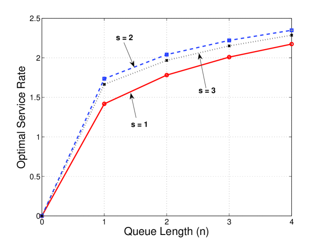
Figure 2 shows that the optimal policy is a non-decreasing function of $n$ for each $s$. It should also be clear that the optimal service rates are non-decreasing in $s$ for each $n$.

Example 3.2.

Consider a phase process with a cyclic transition structure on the set of states $\{1,2,3\}$. See Figure 1(b). The infinitesimal generator matrix for the phase process is

$$\mathbf{Q}=\left[\begin{matrix}-1&1&0\\ 0&-1&1\\ 1&0&-1\end{matrix}\right]$$

and the arrival rates are $\lambda_{1}=0.5,\lambda_{2}=1$ and $\lambda_{3}=1.25$. Figure 3 shows that the optimal policy is non-decreasing in $n$ for each $s$. However, it is clear from this figure that the service rates are not monotone in $s$ when queue length is 4.

In Example 3.2, the phase process transitions from the highest arrival intensity state, 3, to the lowest arrival intensity state, 1. This causes the optimal service rate to be higher in state 2 as compared to state 3 for some congestion levels and thereby renders an optimal policy that is not monotone in $s$. These examples beg the question, is there a reasonable assumption under which the optimal policy is monotone in $s$? Stochastic monotonicity of the phase transition process is one such assumption.

3.2.1 Stochastic Monotonicity for Continuous Time Markov Chains

Intuitively, stochastic monotonicity means that given the arrival process is in a high arrival intensity state, the future states it will encounter are in some sense worse (in terms of arrival intensity) than if the process is in a low arrival intensity state. This leads to the following definitions (see for example Keilson and Kester [16]).

Definition 3.2.

Given two probability vectors p and q, a stochastic matrix M and a homogeneous Markov chain $\{X(t),t\geq 0\}$ with probability transition function $\textbf{P}(t)=\textbf{P}_{ij}(t)$.

1. p stochastically dominates q (p$\geq_{st}$q) iff $\sum_{i=n}^{N}p_{i}\geq\sum_{i=n}^{N}q_{i}$, $n=1,2,\dots$.

2. Letting $\mathbf{M}^{i}$ denote the $i^{th}$ row of the matrix, M is called stochastically monotone if $\mathbf{M}^{k}\geq_{st}\mathbf{M}^{l}$, whenever $k>l$.

3. $\{X(t),t\geq 0\}$ is said to be stochastically monotone if $\textbf{P}(t)$ is monotone.

Note that the transition structure shown in Example 3.1 is stochastically monotone while that for Example 3.2 is not (this is trivial to see once the underlying Markov Chain is uniformized). Some useful stochastic processes that have the stochastic monotonicity property include the birth-death process, the simple random walk, the age of renewal process with decreasing failure rate [16]. In particular, the simple 2-state MMPP fluctuating between high arrival rate and low arrival rate considered by Gupta [13] and Shah-Heydari [24], is also stochastically monotone. The following provides alternative methods for specifying when a transition matrix is stochastically monotone (again refer to Keilson and Kester [16]).

Proposition 3.3.

For monotone matrices the following are equivalent.

1. M is monotone.

2. $(\mathbf{T}^{-1}\mathbf{M}\mathbf{T})_{ij}\geq 0$ where T is a square matrix with 1’s on or below the diagonal.

3. pM$\geq_{st}$qM for all probability vectors p,q with p$\geq_{st}$q.

4. Mv is non-decreasing for all non-decreasing vectors v.

Since for a continuous-time Markov chain with generator matrix $\mathbf{Q}$, stochastic monotonicity implies that the generator for the phase process satisfies the property $(\textbf{T}^{-1}\textbf{Q}\textbf{T})_{ij}\geq 0,i\neq j$ where T is a square matrix with 1’s on or below the diagonal([16]). Choosing a uniformizing constant $\bar{\eta}$ yields $(\textbf{T}^{-1}(\bar{\eta}\textbf{I}+\textbf{Q})\textbf{T})\geq 0$ in all elements. Thus using the second and fourth parts of Proposition 3.3 we have that Q is such that $\bar{\textbf{Q}}:=\bar{\eta}\textbf{I}+\textbf{Q}$ satisfies the property that $\bar{\textbf{Q}}\textbf{v}$ is non-decreasing for all non-decreasing vectors v. This leads to the next result; the main result of this section.

Theorem 3.4.

Suppose that the phase transition process is stochastically monotone.

1. For each $n\in\mathbb{Z}^{+}$, $y_{\alpha,k}(n,s)$ is non-decreasing function of $s$.

2. There exists a discounted cost optimal policy, $\mu_{\alpha}(n,s)$, that is non-decreasing in $s$ for each $n$.

3. Under the assumptions that the holding cost is non-decreasing and convex with polynomial rate of growth and (2.5) hold, there exists an average cost optimal policy $\mu(n,s)$, that is non-decreasing in $s$ for each $n$.

Proof.

We show the first result by induction. The second and third results follow in an analogous manner to Proposition 3.1. The statement holds trivially for $k=0$. Assume it holds for $k$. Using the definitions $\nu=\lambda_{L}+\bar{\eta}+\bar{u}$ and $\bar{\textbf{Q}}=\bar{\eta}\textbf{I}+\textbf{Q}$ we have for $s>1$

$$(\alpha+\nu)\left(y_{\alpha,k+1}(n+1,s)-y_{\alpha,k+1}(n+1,s-1)\right)$$

$$\quad=\phi\left(y_{\alpha,k}(n,s)\right)-\phi\left(y_{\alpha,k}(n,s-1)\right)+\lambda_{s}\left(y_{\alpha,k}(n+2,s)-y_{\alpha,k}(n+2,s-1)\right)$$

$$\qquad+(\lambda_{s}-\lambda_{s-1})\left(y_{\alpha,k}(n+2,s-1)-y_{\alpha,k}(n+1,s-1)\right)$$

$$\qquad+(\lambda_{L}-\lambda_{s})\left(y_{\alpha,k}(n+1,s)-y_{\alpha,k}(n+1,s-1)\right)$$

$$\qquad+\left[\bar{u}\left(y_{\alpha,k}(n+1,s)-y_{\alpha,k}(n+1,s-1)\right)\right.$$

$$\qquad\left.-\left(\phi(y_{\alpha,k}(n+1,s))-\phi\left(y_{\alpha,k}(n+1,s-1)\right)\right)\right]$$

$$\qquad+\bigg{[}\sum_{s^{\prime}=1}^{L}\bar{Q}_{s,s^{\prime}}y_{\alpha,k}(n+1,s^{\prime})-\sum_{s^{\prime}=1}^{L}\bar{Q}_{s-1,s^{\prime}}y_{\alpha,k}(n+1,s^{\prime})\bigg{]}$$ (3.5)

Note that the inductive hypothesis implies that the first four terms in the RHS of (3.2.1) are non-negative. Now as $\phi(y)=\int_{0}^{y}\psi(x)dx$ and $\psi(y)\leq\bar{u}$,

$$\phi(y_{\alpha,k}(n+1,s))-\phi(y_{\alpha,k}(n+1,s-1)) =\int_{y_{\alpha,k}(n+1,s-1)}^{y_{\alpha,k}(n+1,s)}\psi(x)dx$$

$$\leq\bar{u}(y_{\alpha,k}(n+1,s)-y_{\alpha,k}(n+1,s-1)).$$

So the next to last term in RHS of (3.2.1) is non-negative. Furthermore, since the inductive hypothesis and the assumption on $\bar{Q}$ implies the last term in the RHS of (3.2.1) is non-negative. Thus, we conclude from the induction hypothesis that

$$(\alpha+\nu)(y_{\alpha,k+1}(n+1,s)-y_{\alpha,k+1}(n+1,s-1))\geq 0,$$

as desired.  

4 Numerical Study

This section provides two insights using numerical examples. First, we compare the optimal control policy with two natural heuristics. When the environment is changing, it seems a decision-maker that is not armed with the current research might take one of two courses. (S)he might choose to ignore the state change of the environment altogether, or she might treat each state change as permanent and react accordingly. In either case, the resulting control policies are heuristics when compared to the optimal control that takes into account both the phase and queue length processes. The first goal is then to compare the optimal policy with these heuristics. Second, as alluded to in Section 1, the current model can act as a heuristic itself when compared to a model with NHPP arrivals. We analyze when this is a reasonable approximation.

4.1 Comparison with Heuristics

In this section we present a comparison of the performance of optimal policy with several heuristics. Furthermore, we compare the optimal cost achievable with state-dependent service rates with the optimal cost achievable when the service rate is fixed for all states. As mentioned in George and Harrison [11], the difference between these costs represent the economic value of a responsive mechanism. The first heuristic that we consider uses the optimal control for an average cost problem where the arrival process is Poisson with the long-run mean arrival rate of the MMPP. When applied to the original model, this policy is a function of the queue length only. We call this heuristic the Average Rate Method (ARM).

Since the state of the arrival process is known, the decision-maker may solve the stationary model with each potential arrival rate and change the service rate according to the current state of the arrival process. That is to say, a second heuristic is derived in the following way:

1. Compute the service rate control average cost optimal policy, $\pi^{h}_{s}$, for a system with Poisson arrivals with rate $\lambda_{s}$ for each intensity level $s\in\mathcal{S}$.

2. The heuristic for the Markov-Modulated queue is obtained by using $\pi^{h}_{s}$ when the state of the process is $(n,s)$.

This heuristic is referred to as the Phase Rate based Method (PRM). Note that the long-run average arrival rate used in computing the ARM policy is influenced by both the infinitesimal generator matrix and the arrival rates of the phase process while the PRM policy relies only on the arrival rates.

When the service rate is fixed for all states (open loop policy), the queue operates as an MMPP/M/1 queue. For a given service rate, the transition matrix and corresponding steady state distribution can be computed numerically. Based on the steady state distribution one can determine the long-run average cost corresponding to that service rate. We then use a 1-D search procedure to find the service rate that minimizes long-run average cost. This is called the Fixed Rate policy.

A numerical study comparing the performance of these heuristics for various test cases is provided in Examples 4.1 and 4.2. In all cases, the policies and average cost are computed using value iteration where the queue length is truncated at 50. We use the cost rate function $c(\mu)=e^{\mu}-1$ and holding cost rate $h(n)=n$. Service rates are allowed to be chosen from $\mathbb{A}=[0,15]$. In each case the arrival rates change in accordance with the phase state $\{1,2,\ldots,8\}$ with the arrival rates as shown in Table 1.

	Arrival Rate in Phase State
Case	1	2	3	4	5	6	7	8
I	0.1	0.35	0.6	0.85	1.1	1.35	1.6	1.85
II	0.1	0.6	1.1	1.6	2.1	2.6	3.1	3.6
III	0.1	0.85	1.6	2.35	3.1	3.85	4.6	5.35

Table 1: Arrival Rate Parameters for Phase Transition Process in Examples 4.1 and 4.2

Example 4.1.

Suppose that phase process is a birth and death process on states $\{1,2,\dots,8\}$ (recall Figure 1(a)). Fix $c>0$. The transition rates for the phase process are $\eta_{i,i+1}=\eta_{i,i-1}=c$ for $2\leq i\leq 7$, $\eta_{1,2}=c$ and $\eta_{8,7}=c$. A higher value for $c$ means that the phase process transitions faster between the arrival phases. We refer to $c$ as the fluctuation rate scaling parameter. For numerical analysis, we consider three sets of arrival rates for the phase process as shown in Table 1. For each set, the parameter $c$ takes values $0.25,0.50,0.75$ and $1.00$ resulting in a total of 12 different scenarios for the arrival process. Table 2 shows the results for all heuristics.

Scenarios		Gain (% Sub-Optimal)
Arrival Rates	$c$	Optimal	ARM	PRM	Fixed Rate
Case I	0.25	4.3651	4.4650 (2.29 %)	4.3676 (0.06 %)	7.6841 (76.03 %)
	0.50	4.3196	4.3974 (1.80 %)	4.3254 (0.13 %)	7.3185 (69.43 %)
	0.75	4.2818	4.3455 (1.49 %)	4.2909 (0.21 %)	7.0223 (64.01 %)
	1.00	4.2494	4.3031 (1.27 %)	4.2618 (0.29 %)	6.8399(60.96 %)
Case II	0.25	15.5713	16.9349 (8.76 %)	15.7936 (1.43 %)	24.8200 (59.41 %)
	0.50	14.8674	15.6939 (5.56 %)	15.2599 (2.64 %)	22.5509 (51.68%)
	0.75	14.3638	14.9444 (4.04 %)	14.8821 (3.61 %)	21.1000(46.9%)
	1.00	13.9776	14.4189 (3.16 %)	14.5924 (4.40 %)	20.1360(44.06%)
Case III	0.25	47.6797	51.9918 (9.04 %)	49.6854 (4.21 %)	61.1588(28.27%)
	0.50	42.3561	44.4741 (5.00 %)	45.7978 (8.13 %)	55.8678 (31.9%)
	0.75	39.2816	40.6579 (3.51 %)	43.7541 (11.39 %)	51.8600 (32.02%)
	1 .00	37.2150	38.2310 (2.73 %)	42.3809 (13.88 %)	48.9160 (31.44%)

Table 2: Average Cost Rates and Percentage Difference between Optimal and Heuristic Policies for Example 4.1.

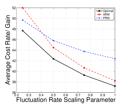
A few observations are in order. Ignoring the dynamic state information of the phase process (and using the ARM policy) is more costly when the fluctuation parameter is lower. This stands to reason since the phase process can be in a state for a long period of time, while the ARM policy assumes the arrival rate is the mean arrival rate. In Case III, when the arrival rate change is the most between phase states and with the slowest rate of changing states, the percent sub-optimality for ARM is above 9%. If we try to approximate the state changes with stationary processes (using PRM) we see that again, the percent sub-optimality is high (above 13%) but this time when the fluctuation parameter is highest.

(a) Small Difference in Phase Intensities (Case I)

(b) Med. Difference in Phase Intensities (Case II)

(c) Large Difference in Phase Intensities (Case III)

(d) Heuristic Vs Opt. Policy (Case III, $n=2$)

Figure 4: Comparison of Gain Values for Heuristic and Optimal Policies for Example 4.1

.

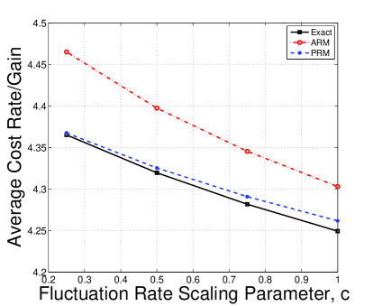
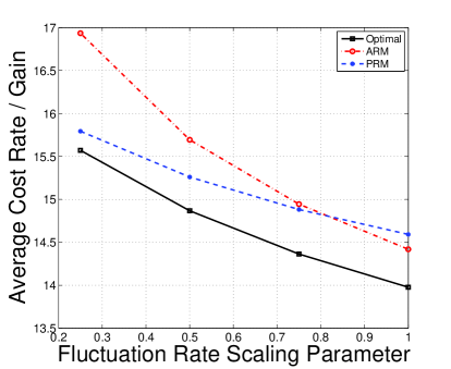
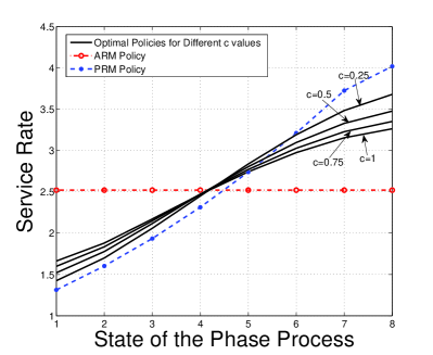
Figures 4(a)-4(c) show the change in the average cost rate under the heuristic and optimal policies as a function of the parameter $c$ for the three arrival cases. Figure 4(d) shows a comparison of the heuristics and optimal policies for the arrival rates in Case III and $n=2$ for various values of fluctuation rate parameter (the behavior is similar for other values of $n$). It should be clear that the PRM policy outperforms the ARM policy in most cases except for high values of $c$ in Case III. Moreover, one should note that the performance of the ARM policy improves while that of PRM policy degrades in comparison to the optimal policy as the fluctuation rate parameter increases. Intuitively this seems reasonable since for low values of $c$ the phase process spends more time in each phase. Therefore the PRM policy, that in each phase applies the optimal policy for a stationary M/M/1 queue with arrival rate of that particular phase, performs better than the ARM policy. In fact, if $c=0$, the PRM policy is optimal since the phase process is stationary with the arrival rate of initial phase.

At high values of $c$ (since the system sees more and more transitions), the arrival process behaves like a Poisson process with the average arrival rate of MMPP. Therefore the PRM policy gets penalized more in comparison to the ARM policy in this case. In Figure 4(d) we also see that the change in the optimal service rates as a function of phase state for each congestion level is lower for higher values of $c$.

Example 4.2.

In this example we study a cyclic phase process (cf. Figure 1(b)) on the states $\{1,2,\dots,8\}$. The transition rates for the phase process are $\eta_{i,i+1}=c$ for $1\leq i\leq 7$ and $\eta_{8,1}=c$. Similar to the previous example we perform the numerical analysis for 12 scenarios for the phase process; three different sets of arrival rates given in Table 1 and for each set of arrival rates, $c$ takes values $0.25,0.50,0.75$ and $1.00$.

Scenarios		Gain (% Sub-Optimal)
Arrival Rates	$c$	Optimal	ARM	PRM	Fixed Rate
Case I	0.25	4.1872	4.2295 (1.01 %)	4.2267 (0.94 %)	6.3440 (51.51%)
	0.50	4.0603	4.085 (0.61 %)	4.1204 (1.48 %)	5.9620 (46.84%)
	0.75	3.988	4.0051 (0.43 %)	4.0574 (1.73 %)	5.7700 (44.68%)
	1.00	3.9423	3.9549 (0.32 %)	4.0166 (1.89 %)	5.6647 (43.69%)
Case II	0.25	12.894	13.2042 (2.41 %)	13.9767 (8.39 %)	17.2439 (33.74 %)
	0.50	11.9656	12.1319 (1.39 %)	13.2268 (10.54 %)	15.6149 (30.5 %)
	0.75	11.5435	11.6531 (0.95 %)	12.8573 (11.38 %)	14.9350 (29.38 %)
	1.00	11.2996	11.3786 (0.70 %)	12.6374 (11.84 %)	14.51 (28.43 %)
Case III	0.25	31.2724	32.1887 (2.93 %)	39.4752 (26.23 %)	35.5711 (13.75 %)
	0.50	28.3046	28.7893(1.71 %)	37.1449 (31.23 %)	33.8800 (19.7 %)
	0.75	27.0506	27.3664 (1.16 %)	36.0660 (33.33 %)	32.7185 (20.95%)
	1.00	26.3445	26.5702 (0.86 %)	35.4401 (34.53 %)	31.9436 (21.25 %)

Table 3: Average Cost Rates and Percentage Difference between Optimal and Heuristic Policies for Example 4.2

(a) Small Difference in Phase Intensities (Case I)

(b) Med. Difference in Phase Intensities (Case II)

(c) Large Difference in Phase Intensities (Case III)

(d) Heuristic Vs Optimal Policy (Case III, $n=2$)

Figure 5: Comparison of Gain Values for Heuristic and Optimal Policies for Example 4.2

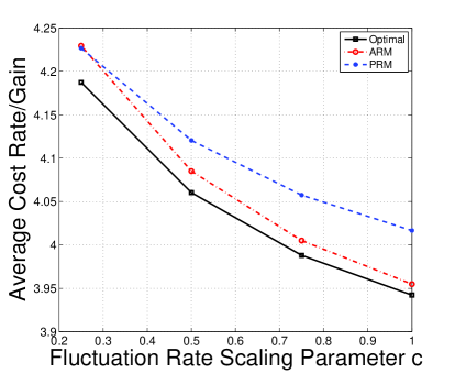
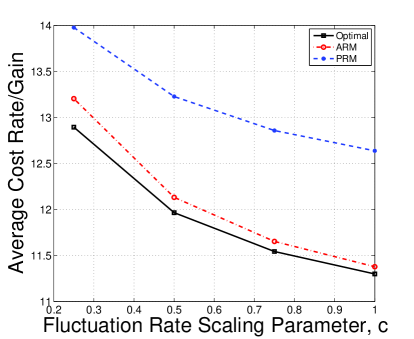
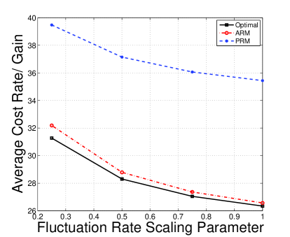
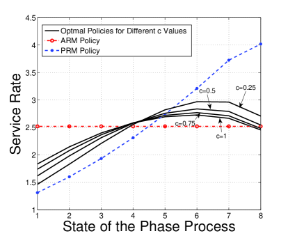
Figures 5(a)-5(c) show the change in the average cost computed under the heuristics as well as the optimal policies as a function of parameter $c$ for the three arrival cases. It is interesting to observe that unlike Example 4.1, the ARM policy outperforms the PRM policy in almost all cases. As illustrated in Example 3.2, when the phase process has cyclic transitions, the optimal service rates may not be monotone in the phase process (for each fixed $n$). In fact, while the service rates for the PRM policy are monotone in the phase of the transition process for each congestion level, the service rates in the optimal policy may begin to decrease as the phase state increases. This can be more clearly observed in Figure 5(d) which shows a comparison of heuristic and optimal policies as a function of the phase state when $n=2$ for various values of parameter $c$ and the arrival rates of Case III. Thus the ARM policy approximates the optimal policy better than the PRM policy which explains the observed performance difference.

Similar to the previous example, we observe that the performance of the ARM policy gets worse and that of PRM policy improves with a decrease in the fluctuation rate parameter $c$. Furthermore, the average cost percent differences provided in Table 3 show that the ARM policy performs extremely well for all three arrival rate cases (less than 5% from optimal for all cases). The PRM policy performs well for Case I but the degradation in its performance is quite significant (almost 35 % from optimal for Case III with $c=1$) when the difference in arrival rates is medium or high (Cases II and III).

Tables 2 and 3 show the optimal costs achievable under the fixed rate mechanism under the column heading “fixed rate”. We find that costs are between 13% and 76% suboptimal when using a fixed rate mechanism relative to the variable rate mechanism. This shows that there is substantial benefit in investing in a responsive mechanism. Furthermore, these examples show that one cannot rely on a particular heuristic method to perform well in all scenarios. In particular, we find that within the gamut of simple heuristic methods considered here, the transition structure and the transition rates of the phase process play an important role in the selection of an appropriate approximation method.

4.2 Approximation of a System with Non-homogeneous Poisson Arrivals

When the arrival process follows known rate changes, a non-homogeneous Poisson process is a reasonable modeling tool. In the classical work of Green and Kolesar [12] or Massey and Whitt [19] the analysis of queues with non-stationary arrivals is considered. From the standpoint of control, Yoon and Lewis [27] consider the case of admission and pricing control. One thing is certain from Yoon and Lewis’s work, control of non-stationary processes can be computationally intensive. This is due the fact that to solve each instance the numerical approach requires the time to be discretized.

In this section we explore the possibility of computing an approximate average cost optimal policy for a single server queue with non-homogeneous Poisson arrivals using the optimal policies for a system with a “suitable” Markov-modulated Poisson arrival process. Apart from the arrival process, other details are the same as the setting described in Section 2. Let the arrival process be an NHPP with rate $\lambda(t)$. Assume that $\lambda(t)$ is a periodic function with period $T$. Since the optimization criterion considered in this study is over an infinite time horizon, and the rate function for NHPP is a periodic function of time, the principle of optimality implies that only the time elapsed in the current period and the number of jobs in the system need to be included in the state space [27].

To compute the optimal policy for an NHPP arrival process numerically, the time period is divided into $n$ equally spaced segments of length $\Delta t=T/n$. Denote the state space for this discretized process as $\mathbb{X}=\{(n,z)\mid n\in\mathbb{Z}^{+},s\in\{0,\Delta t,\dots,T-\Delta t\}\}$. Under this setting, the decision epochs are the time points $0,\Delta t,2\Delta t,\dots,T-\Delta t$. Let $\nu$ be a uniformizing rate of the process. An event (arrival, departure or dummy transition) occurs at a decision epoch with probability $1-e^{-\nu\Delta t}$ and with probability $e^{-\nu\Delta t}$ no event occurs. The standard theory of Markov decision processes yields the following average cost optimality inequality (ACOI):

$$w(n,z) \geq\min_{x\in\mathbb{A}}\bigg{\{}\left(-g+h(n)+\mathbf{1}_{\{n>0\}}c(x)\right)\Delta t+(1-e^{-\nu\Delta t})\bigg{(}\frac{\lambda(z)}{\nu}w(n+1,z+\Delta t)$$

$$\qquad{}+\mathbf{1}_{\{n>0\}}\frac{x}{\nu}w(n-1,z+\Delta t)+\big{(}1-\frac{\lambda(z)}{\nu}-\mathbf{1}_{\{n>0\}}\frac{x}{\nu}\big{)}w(n,z+\Delta t)\bigg{)}$$

$$\qquad{}+e^{-\nu\Delta t}w(n,z+\Delta t)\bigg{\}}\text{ for }n\in\mathbb{Z}^{+},z=0,\Delta t,\dots,T-2\Delta t,\text{ and}$$

$$w(n,T-\Delta t)\geq \min_{x\in\mathbb{A}}\bigg{\{}\left(-g+h(n)+\mathbf{1}_{\{n>0\}}c(x)\right)\Delta t+(1-e^{-\nu\Delta t})\bigg{(}\frac{\lambda(T-\Delta t)}{\nu}w(n+1,0)$$

$$\qquad{}+\mathbf{1}_{\{n>0\}}\frac{x}{\nu}w(n-1,0)+\big{(}1-\frac{\lambda(z)}{\nu}-\mathbf{1}_{\{n>0\}}\frac{x}{\nu}\big{)}w(n,0)\bigg{)}$$

$$\qquad{}+e^{-\nu\Delta t}w(n,0)\bigg{\}}\text{ for }n\in\mathbb{Z}^{+},$$

where $\mathbf{1}_{E}$ is the indicator function of the event $E$. When the solution, $(w,g)$ to the ACOI exists, $w$ is called the relative value function and $g^{\ast}(x)=g$ is the optimal long-run expected average cost for any initial state $x$.

We now present a method for constructing an approximate policy for NHPP arrivals. The main idea is to approximate the NHPP by an appropriately constructed MMPP. This is done by dividing the time period $T$ into $l$ subintervals and constructing an MMPP with the same number of phases as the number of subintervals i.e, $l$. We choose a cyclic transition structure for the phase process with arrival rate in each phase as the average rate over that subinterval. Transition rates for the phase process can be selected such that the mean sojourn time in phase $s$ is the width of the corresponding interval. The optimal policy corresponding to this MMPP can then be applied to the original NHPP arrivals. The detailed procedure to evaluate the approximate policy is described below:

1. Partition the interval $[0,T]$ into $l$ subintervals, $[t_{s-1},t_{s}]$, $s=1,\dots,l$ with $t_{0}=0$ and $t_{l}=T$.

2. Compute average rates over each partition,

   $$\lambda_{s}=\frac{\int_{t_{s-1}}^{t_{s}}\lambda(t)dt}{(t_{s}-t_{s-1})}.$$

3. Compute transition rates, $\eta_{i,j}$, for the phase process of MMPP,

   $$\eta_{i,j}=\left\{\begin{array}[]{lll}\frac{1}{(t_{i}-t_{i-1})},&1\leq i\leq l-1,j=i+1\hbox{;}\\ \frac{1}{(t_{l}-t_{l-1})},&i=l,j=1\hbox{;}\\ 0,&\hbox{otherwise}\end{array}\right\}$$

   .

4. Compute the optimal policy corresponding to the MMPP arrival process constructed in previous steps. Denote this policy as $\mu(n,s)$ , $n\in\mathbb{Z}^{+},s\in{1,2,\dots,l}$.

5. Construct the approximate policy, $\hat{\mu}$, for the NHPP process as

   $$\hat{\mu}(n,t)=\mu(n,s)\text{ for }t_{s-1}\leq t\leq t_{s}\text{ , }n=0,1,2,\dots.$$

A numerical study comparing the performance of the approximation procedure stated above for various test cases is provided in Examples 4.3 and 4.4. In all cases, the policies and average cost are computed using value iteration where the queue length is truncated at 50 to keep the size of the state space manageable.

Example 4.3.

In this example, we consider a NHPP with the following (periodic) rate function,

$$\lambda(t) =\begin{cases}0.1\text{\quad for\quad}0\leq t<T/5\\ 2.0\text{\quad for\quad}T/5\leq t<2T/5\\ 4.0\text{\quad for\quad}2T/5\leq t<3T/5\\ 2.0\text{\quad for\quad}3T/5\leq t<4T/5,\\ 0.1\text{\quad for\quad}4T/5\leq t<T,\\ \end{cases}$$

where $T$ is the time period of the rate function. One can think of this rate function as a quantized version of a triangular waveform with time period $T$. The discretization interval $\Delta t$, for solving the problem with NHPP arrivals is selected as $0.05$ units. The cost rate function is $c(\mu)=e^{\mu}-1$ and holding cost function is $h(n)=n$. Service rates can be selected from a set $\mathbb{A}=[0,10]$. For computing the approximate policy, we partition the interval $[0,T]$ into 5 subintervals of equal length. Thus, the arrival rates for the corresponding MMPP are $\lambda_{1}=0.1,\lambda_{2}=2.0,\lambda_{3}=4.0$,$\lambda_{4}=2.0$ and $\lambda_{5}=0.1$ and the associated generator matrix is

$$\mathbf{Q} =\frac{5}{T}\left[\begin{matrix}-1&1&0&0&0\\ 0&-1&1&0&0\\ 0&0&-1&1&0\\ 0&0&0&-1&1\\ 1&0&0&0&-1\end{matrix}\right],$$

Figure 6: NHPP Policy vs Approximate MMPP policy for various congestion levels (T=7)

Time Period $(T)$	Gain(% Sub-Optimal)
	Optimal	App. MMPP
4	8.5667	8.5932 (0.31%)
5	8.7750	8.7262 (0.41%)
6	8.7467	8.7925 (0.52%)
7	8.8225	8.8785 (0.64%)

Table 4: Average Cost Rates and Percentage Difference between Optimal and Approximate NHPP Policy

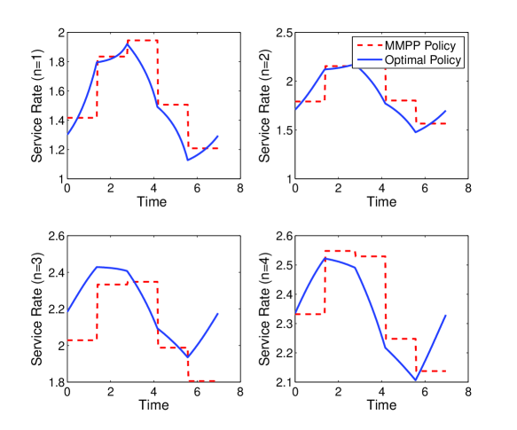
Figure 6 show a comparison of optimal policy with approximate MMPP policy. Table 4 gives the average cost percent difference between the performance of approximate and optimal policy for various test scenarios. This data shows that the approximate policies perform extremely well in all cases (less than 1% sub-optimal).

Example 4.4.

In this example, we consider a NHPP with the following (periodic) rate function,

$$\lambda(t) =5sin(\omega T)+6$$

where $T$ is the time period of the rate function and $\omega=\frac{2\pi}{T}$ the frequency. We consider the cases in which $T$ is set to $\frac{n\pi}{2},n=1,2,3,\text{and},4$. The discretization interval $\Delta t$, for solving the problem with NHPP arrivals is selected as $\frac{T}{200}$ units. The cost rate function is $c(\mu)=\frac{\mu^{2}}{2}-1$ and holding cost function is $h(n)=(n-20)^{+}$. Service rates can be selected from a set $\mathbb{A}=[0,15]$. For computing the approximate policy, we partition the interval $[0,T]$ into 6 subintervals of equal length.

Figure 7: NHPP Policy vs Approximate MMPP policy for various congestion levels $(T=\frac{3\pi}{2})$

Time Period $(T)$	Gain(% Sub-Optimal)
	Optimal	App. MMPP
$\frac{\pi}{2}$	18.90	19.38 (2.52%)
$\pi$	18.91	19.32 (2.21%)
$\frac{3\pi}{2}$	18.93	19.08 (0.82%)
$2\pi$	18.94	19.29 (1.84%)

Table 5: Average Cost Rates and Percentage Difference between Optimal and Approximate NHPP Policy

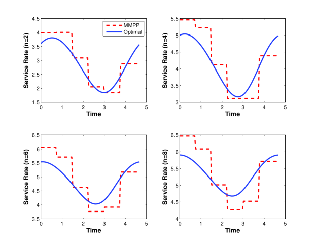
Figure 7 shows a comparison of the optimal policy with heuristic MMPP policy. Table 5 gives the average cost percent difference between the performance of approximate and optimal policy for various test scenarios. We can again see that the approximate policies perform well in all cases (less than 3% sub-optimal).

Of course, we can not conclude from this limited analysis that MMPP approximate policies will perform well for NHPP in more general settings. Our motivation in presenting this analysis is to stimulate further research in this direction.

5 Conclusions

In this paper we investigate the problem of service rate control for a single server queue with non-stationary arrivals. We propose a framework based on the Markov modulated Poisson processes; a popular model amongst practitioners that is also relatively easy to analyze. Assuming that the goal is to minimize a combination of effort cost and holding cost incurred per unit time, we study this problem under both the discounted and average cost optimality criterion. In either case, we characterize the structure of an optimal service rate as being monotone in the queue length for each arrival rate but not necessarily monotone in the arrival rates for each queue length. In particular, we show that the manner in which the process switches between the arrival rates plays an important role in determining the structure of the optimal policy. We further prove that monotonicity in the arrival rates is recovered when the transition matrix governing the MMPP is stochastically monotone.

There are several ways to extend our work. Our numerical study confirms that in some cases simple heuristics may perform well in the face of changing arrival rates. However, it also points out that careful selection based on the parameters of the system is required, and in many cases applying the proposed model is essential (as opposed to the heuristics). The second part of our numerical work points to the fact that our model can be used as a heuristic itself. We show that we can potentially provide a policy for a system with non-homogenous Poisson arrivals using the optimal policy for an MMPP/M/1 queue. Our results indicate that this may be a promising direction for future research.

Another problem of interest is that of the control of MMPP/M/1 queue with a finite buffer but with an explicit constraint on the job loss rate. Under this setting, while the technical conditions required for stability are not needed, handling the explicit constraint poses a significant challenge. We note that results provided by Ata [1] for the stationary arrival case may be useful.

The model under study assumes that complete information about arrival statistics is available. This may be unreasonable in situations where arrival statistics cannot be associated with the observable features of the system. A promising direction of work may be to tackle such situations using the partially observable Markov decision process framework.

Finally, we would like to point out that although for ease of exposition, we assume that the cost of effort function, $c(\mu)$, is strictly convex, continuously differentiable and non-decreasing, our proofs (with minor modification) and results hold for more general cost of effort functions. Using the analysis presented by George and Harrison [11], it can be easily shown that the structural results for an optimal policy continue to hold when $c(\mu)$ is assumed to be non-decreasing and continuous.

6 Appendix

This appendix is dedicated to providing proofs of Propositions 2.1 and 2.2. The results of Dai [7] and Dai and Meyn [8] are utilized to show the stability of a stochastic model by establishing the stability of its fluid limit approximation. For the purpose of this analysis, consider the continuous time Markov process, $X^{\pi}(t)=\{(Q^{\pi}(t),S^{\pi}(t)),t\geq 0\}$, induced by an admissible stationary policy $\pi\in\Pi$ where $\{Q^{\pi}(t),t\geq 0\}$ and $\{S^{\pi}(t),t\geq 0\}$ represent the queue length and phase transition process for arrivals, respectively.

The proof approach for Proposition 2.1 follows closely that of Kaufman and Lewis [15] (Proposition 3.1) and is done in several steps. Let $\hat{\pi}$ be a policy that selects a constant rate $\hat{\mu}\in(\sum_{s=1}^{L}p_{s}\lambda_{s},\bar{u}]$ whenever the queue is non-empty. Let $X^{\hat{\pi}}(t)=\{(Q^{\hat{\pi}}(t),S^{\hat{\pi}}(t)),t\geq 0\}$ be the Markov process induced by the policy $\hat{\pi}$ on state space $\mathbb{X}=\{(n,s)\mid n\in\mathbb{Z}^{+},s\in\mathcal{S}\}$. Since the policy is fixed for the remainder of this section, in the interest of brevity we suppress dependence on $\hat{\pi}$. The norm of a state, $x=(n,s)\in\mathbb{X}$, is defined to be $\lvert x\rvert:=n+s$. For an initial state $X(0)=x$, we define the scaled queue length process

$$\bar{Q}^{x}(t) :=\frac{1}{\lvert x\rvert}Q^{x}(\lvert x\rvert t).$$

We will use a similar notation to denote scaled versions of other stochastic processes.

For each $s\in\mathcal{S}$, let $\{\xi_{s}(k),k\geq 1\}$ be a sequence of i.i.d exponential random variables with mean $1/\lambda_{s}$. The sequence $\{\xi_{s}(k),k\geq 1\}$ represents the set of job inter-arrival times when the arrival process is in phase $s$. Also, let $\{\eta(k),k\geq 1\}$ be a sequence of i.i.d exponential random variables with mean $1$ representing the set of job completion times. Based on these sequences, we define the following cumulative processes

$$E_{s}(t) =\max\{k\geq 0\mbox{{\bf$\ \mid\ $}}\xi_{s}(1)+\xi_{s}(2),\dots,\xi_{s}(k)\leq t\}\qquad\text{for $s\in\mathcal{S}$},$$

$$D(t) =\max\{k\geq 0\mbox{{\bf$\ \mid\ $}}\eta(1)+\eta(2),\dots,\eta(k)\leq t\}.$$

Let $Y^{x}_{s}(t)$ be the cumulative amount of time the arrival process spends in phase $s$ until time $t$ when the initial state is $x$. Similarly, let $T^{x}(t)$ be the cumulative amount of time for which there is at least one customer in the queue, $I^{x}(t)$ be the cumulative amount of time when the queue is empty and $W^{x}(t)$ be the total work done by the server until time t. We can now write the following system of equations for the stochastic process induced by policy $\hat{\pi}$ when starting from initial state $x$,

$$Q^{x}(t)=Q^{x}(0)+\sum_{s=1}^{L}E_{s}(Y^{x}_{s}(t))-D(W^{x}(t)),$$ (6.1)

$$Q^{x}(t)\geq 0,$$ (6.2)

$$\sum_{s=1}^{L}Y_{s}^{x}(t)=t,$$ (6.3)

$$W^{x}(t)=\hat{\mu}T^{x}(t),$$ (6.4)

$$T^{x}(t)+I^{x}(t)=t,$$ (6.5)

$$\int_{0}^{\infty}Q^{x}(t)dI^{x}(t)=0,$$ (6.6)

$$Y^{x}_{s}(t),T^{x}(t),I^{x}(t),W^{x}(t)\quad\text{start from zero and are non-decreasing in $t$.}$$ (6.7)

A few comments are in order. First, note that (6.6) imposes the constraint that the server is idle only when the system is empty. For a subsequence $\{x_{n},n\geq 1\}$ such that $|x_{n}|\rightarrow\infty$, any limit point, $\bar{Q}(t)$, of the sequence $\{\bar{Q}^{x_{n}},n\geq 1\}$ is called a fluid limit. It will be shown that every fluid limit satisfies a set of equations known as the fluid model. A fluid model is called stable if there exists a $t_{0}>0$ such that $\bar{Q}(t)=0$ for all $t\geq t_{0}$ and for all fluid limits. We next present the fluid model and convergence results for the scaled processes

Proposition 6.1.

Let $\{x_{j}\mbox{{\bf$\ \mid\ $}}x_{j}\in\mathbb{X},j\geq 1\}$ be a sequence of initial states with $\lvert x_{j}\rvert\rightarrow\infty$. Then with probability 1, there exists a subsequence, $\{x_{j_{k}},k\geq 1\}$, such that

$$(\bar{Q}^{x_{j_{k}}}(0),\bar{S}^{x_{j_{k}}}(0))\rightarrow(\bar{Q}(0),0),$$ (6.8)

$$(\bar{Q}^{x_{j_{k}}}(t),\bar{T}^{x_{j_{k}}}(t))\rightarrow(\bar{Q}(t),\bar{T}(t))\quad\text{uniformly on compact sets (u.o.c.)},$$ (6.9)

where $(\bar{Q}(t),\bar{T}(t))$ satisfy the following equations,

$$\bar{Q}(t)=\bar{Q}(0)+\sum_{s=1}^{L}p_{s}\lambda_{s}t-\bar{W}(t),$$ (6.10)

$$\bar{Q}(t)\geq 0,$$ (6.11)

$$\bar{W}(t)=\hat{\mu}\bar{T}(t),$$ (6.12)

$$\bar{T}(t)+\bar{I}(t)=t,$$ (6.13)

$$\int_{0}^{\infty}\bar{Q}(t)d\bar{I}(t)=0,$$ (6.14)

$$\bar{T}(t),\bar{I}(t),\bar{W}(t)\quad\text{start from zero and are non-decreasing in $t$}.$$ (6.15)

Proof.

Since $\bar{Q}^{x_{j}}(0)\leq 1$, $\bar{S}^{x_{j}}(0)\leq 1$ and $1\leq S^{x_{j}}(0)\leq L$ for all $j\in\mathbb{N}$, there exists a subsequence, $\{x_{j_{k}},k\geq 1\}$ such that $(\bar{Q}^{x_{j_{k}}}(0),\bar{S}^{x_{j_{k}}}(0))\rightarrow(\bar{Q}(0),0)$. For any fixed sample path $\omega$ and $0\leq s\leq t$, we have $0\leq\bar{T}^{x_{j}}(t)-\bar{T}^{x_{j}}(s)\leq t-s$. Thus, the function $\bar{T}^{x_{j}}(t)$ is uniformly Lipschitz of order 1. Since $0\leq\bar{T}^{x_{j}}(t)\leq t$, it is also uniformly bounded for each $j\geq 1$. Therefore, the sequence $\{\bar{T}^{x_{j}}(t),j\geq 1\}$ is equicontinuous. By Arzela-Ascoli theorem, any subsequence of $\{\bar{T}^{x_{j}}(t),j\geq 1\}$ has a u.o.c. convergent subsequence.

Since the phase transition process is ergodic, for each $s\in\{1,\dots,L\}$ we have with probability 1 $\lim_{t\rightarrow\infty}Y_{s}^{x}(t)/t=p_{s}$. Furthermore, from the strong law of large numbers for renewal processes, the following hold almost surely

$$\lim_{t\rightarrow\infty}E_{s}(t)/t =\lambda_{s}\quad s\in\mathcal{S},$$

$$\lim_{t\rightarrow\infty}D(t)/t =1.$$

The above results can be used in a manner similar to Lemma 4.2 of [7], to yield (with probability 1)

$$\bar{Y}_{s}(t) =\lim_{k\to\infty}\frac{1}{\lvert x_{j_{k}}\rvert}Y^{x_{j_{k}}}(\lvert x_{j_{k}}\rvert t)=p_{s}t\quad u.o.c.,\text{ for $s\in\mathcal{S}$},$$ (6.16)

$$\bar{E}_{s}(t) =\lim_{k\to\infty}\frac{1}{\lvert x_{j_{k}}\rvert}E(\lvert x_{j_{k}}\rvert t)=\lambda_{s}t\quad u.o.c.,\text{ for $s\in\mathcal{S}$}$$ (6.17)

$$\bar{D}(t) =\lim_{k\to\infty}\frac{1}{\lvert x_{j_{k}}\rvert}D(\lvert x_{j_{k}}\rvert t)=t\quad u.o.c.$$ (6.18)

The equality in (6.10) follows from (6.1) and (6.16)-(6.18). Similarly, (6.12)-(6.15) follow directly from (6.4)-(6.7), respectively.  

Proof of Proposition 2.1: We start by showing that the fluid model provided in (6.10)-(6.15) is stable. First note that $\bar{T}(t),\bar{I}(t)\text{ and }\bar{Y}_{s}(t)$ are Lipschitz continuous and therefore absolutely continuous and differentiable almost everywhere. Taking the derivative with respect to $t$ in (6.10) and (6.12) yields

$$\dot{\bar{Q}}(t) =\sum_{s=1}^{L}p_{s}\lambda_{s}-\hat{\mu}\dot{\bar{T}}(t).$$

Further, due to the non-idling constraint (6.14), $\dot{\bar{I}}(t)=0$ whenever $\bar{Q}(t)>0$. Thus, from (6.13), $\dot{\bar{T}}(t)=1$ whenever $\bar{Q}(t)>0$. So for $\bar{Q}(t)>0$, we have

$$\dot{\bar{Q}}(t) =\sum_{s=1}^{L}p_{s}\lambda_{s}-\hat{\mu}.$$

Our choice of the stationary policy enabled by the stability condition (2.5), implies that $\dot{\bar{Q}}(t)<0$ whenever $\bar{Q}(t)>0$. Thus from Lemma 5.2 of [7] we have that the fluid limit process for queue length is non-increasing and there exists a $t_{0}\geq 0$ such that $\bar{Q}(t)=0$ for all $t\geq t_{0}$. That is, the fluid model is stable. The results of Theorem 4.2 of [7] imply that the Markov process induced by the stationary policy $\hat{\pi}$, is positive recurrent and stationary distribution exists. Furthermore, since the embedded discrete time Markov chain for the process is irreducible, this process is ergodic. This implies that the long-run average cost under $\hat{\pi}$, say $g^{\hat{\pi}}$, is independent of the initial state.

To show that $g^{\hat{\pi}}$ is finite, we use the results of Theorem 4.1(i) of [8]. Since the fluid model is stable and conditions A1) and A2) of Theorem 4.1 hold, it follows that for any integer $p\geq 1$ $\lim\sup_{t\rightarrow\infty}\frac{1}{t}\int_{0}^{t}\operatorname{\mathbb{E}}_{x}[|Q(u)|^{p}]du<\infty$ for each initial condition $x$. Since the holding cost has a polynomial rate of growth, we have that the long-run average holding cost rate is finite. Moreover, the direct contribution to long-run cost rate due to serving at $\hat{\mu}$ whenever the queue is not empty is at most $c(\hat{\mu})<\infty$. It therefore follows $g^{\hat{\pi}}$ is finite.

It remains to consider the necessity of (2.5). Consider the Markov process induced by a policy that uses the highest available service rate whenever the queue is not empty. As shown by Yechiali[26] using the detailed balance equations for the steady state distribution a non-trivial invariant measure exists only if $\bar{u}>\sum_{s=1}^{L}p_{s}\lambda_{s}$. The result follows and the proof is complete.  

The remainder of this section is dedicated to proving Proposition 2.2 holds. We show that the optimal value and relative value functions satisfying the ACOI, (2.2), exist and can be obtained via limits from the discounted expected cost value functions. Thus, the structural results proved for the discounted cost case continue to hold for the average cost case. In proving these results, we verify the following set of assumptions $(SEN)$ (included for completeness) provided by Sennott [23] hold.

• SEN1: There exist $\delta>0$ and $\epsilon>0$ such that for every state and action, there is a probability of at least $\epsilon$ that the transition time will be greater that $\delta$.

• SEN2: There exists $B$ such that $\tau(i,\mu)\leq B$ for every state $i$ and control $\mu$, where $\tau(i,\mu)$ is the expected transition time out of state $i$ when control $\mu$ is chosen.

• SEN3: $v_{\alpha}(i)<\infty$ for all states $i$ and $\alpha>0$.

• SEN4: There exists $\alpha_{0}>0$ and nonnegative numbers $M_{i}$ such that $w_{\alpha}(i)\leq M_{i}$ for every state $i$ and $0<\alpha<\alpha_{0}$ where $w_{\alpha}(i)=v_{\alpha}(i)-v_{\alpha}(\mathbf{0})$, for distinguished state $\mathbf{0}$. For every state $i$, there exists an action $\mu_{i}$ such that $\sum_{j}P_{ij}(\mu_{i})M_{j}<\infty$.

• SEN5: There exists $\alpha_{0}>0$ and a non-negative number $N$ such that $-N\leq w_{\alpha}(i)$ for every $i$ and $0\leq\alpha\leq\alpha_{0}$.

• SEN6: For each state $i$, the expected single stage discounted cost $f_{\alpha}(i,\mu)$ is a lower semi-continuous (lsc) function on the product space $[0,\infty)\times\mathbb{A}$. Note that $f_{0}(i,\mu)$ is the un-discounted single stage cost.

• SEN7: For all states $i$ and $j$, the function $L_{ij}(\alpha,\mu)=P_{ij}(\mu)\int_{t=0}^{\infty}e^{-\alpha t}\nu e^{-\nu t}dt$ is a lsc function on the product space $[0,\infty)\times\mathbb{A}$.

• SEN8: Assume that $\alpha_{n}$ is a sequence of discount factors converging to 0 with the property that $\pi_{\alpha_{n}}$, the associated sequence of $\alpha$-discount optimal policies, converge to a stationary policy $\pi$. Then for each state $i$, $\lim\inf_{n}\tau(i,\pi_{\alpha_{n}})\leq\tau(i,\pi)$.

Proof of Proposition 2.2: We begin by verifying the SEN assumptions. Since the uniformizing rate is strictly positive and finite, assumptions SEN1 and SEN2 hold. It was shown in Proposition 2.1 that under the stability condition (2.5), there exists a stationary policy that induces an ergodic Markov process with finite long-run average expected cost. Thus, the hypotheses of Lemma 2 of [23] hold; validating SEN3 and SEN4 assumptions. Let $\bar{s}=\arg\min_{s\in\mathcal{S}}\{v_{\alpha}(0,s)\}$ and define the distinguished state as $\mathbf{0}=(0,\bar{s})$. It follows from Proposition 3.1 that for any $\alpha>0$, $v_{\alpha}(\mathbf{0})\leq v_{\alpha}(n,s)$ for all $(n,s)\in\mathbb{X}$. Therefore, $w_{\alpha}(n,s)\geq 0$ and SEN5 is satisfied. SEN6 holds since for each $(n,s)\in\mathbb{X}$, $f_{\alpha}((n,s),\mu)=(c(\mu)+h(n))/(\alpha+\nu)$ is a continuous function on $[0,\infty)\times\mathbb{A}$.

There is no decision to be made when $n=0$. Fix $n\geq 1$ and $s\in\{1,2,\dots,L\}$ and note,

$$L_{(n,s),(n^{\prime},s^{\prime})}(\alpha,\mu) =\begin{cases}\frac{\lambda_{s}}{\alpha+\nu}\text{\quad if\quad}n^{\prime}=n+1,s^{\prime}=s,\\ \frac{\mu}{\alpha+\nu}\text{\quad if\quad}n^{\prime}=n-1,s^{\prime}=s,\\ \frac{Q_{ss^{\prime}}}{\alpha+\nu}\text{\quad if\quad}n^{\prime}=n,s^{\prime}\in\mathcal{S},\\ 0\text{\qquad otherwise.\quad}\end{cases}$$ (6.19)

So the function $L_{x,x^{\prime}}(\alpha,\mu)$ is jointly continuous in $\alpha$ and $\mu$ for each $x,x^{\prime}\in\mathbb{X}$, therefore SEN7 holds. Finally, since for any policy $\pi$, $\tau(i,\pi)=1/\nu$, SEN8 holds.

SEN1, SEN3, SEN6 and SEN7 are required in Theorem 11 of [23] to prove the first result. Since the holding costs are assumed to have a polynomial rate of growth, the hypotheses of Proposition 4 of [23] are satisfied. The last two results follow from Theorem 12 (and its proof) of [23].

References

- [1] B. Ata. Dynamic Power Control in a Wireless Static Channel Subject to a Quality-of-Service Constraint. Operations Research, 53(5):842–851, September 2005.
- [2] B. Ata and K. E. Zachariadis. Dynamic power control in a fading downlink channel subject to an energy constraint. Queueing Systems, 55(1):41–69, December 2006.
- [3] R.A. Berry. Power and delay trade-offs in fading channels. PhD Thesis, 2000.
- [4] D.P. Bertsekas. Dynamic Programming and Optimal Control-Vol II. Athena Scientific, 1995.
- [5] S. Boyd and L. Vandenberghe. Convex Optimization. Cambridge University Press, 2004.
- [6] T.B. Crabill. Optimal Control of a Maintenance System with Variable Service Rates. Operations Research, 22(4):736–745, July 1974.
- [7] J.G. Dai. On positive Harris recurrence of multiclass queueing networks: a unified approach via fluid limit models. The Annals of Applied Probability, 40(11):49–77, 1995.
- [8] J.G. Dai and S.P. Meyn. Stability and convergence of moments for multiclass queueing networks via fluid limit models. IEEE Transactions on Automatic Control, 40(11):1889–1904, 1995.
- [9] E.A. Feinberg and M.E. Lewis. Optimality Inequalities for Average Cost Markov Decision Processes and the Stochastic Cash Balance Problem. Mathematics of Operations Research, 32(4):769–783, November 2007.
- [10] V.S. Frost and B. Melamed. Modeling For Telecommunications Networks. IEEE Communications Magazine, (March):70–81, 1994.
- [11] J.M. George and J.M. Harrison. Dynamic Control of a Queue with Adjustable Service Rate. Operations Research, 49(5):720–731, September 2001.
- [12] L.V. Green and P.J. Kolesar. On the accuracy of the simple peak hour approximation for Markovian queues. Management science, 41(8):1353–1370, 1995.
- [13] V. Gupta, M. Harchol-Balter, A. Scheller Wolf, and U. Yechiali. Fundamental characteristics of queues with fluctuating load. ACM SIGMETRICS Performance Evaluation Review, 34(1):203, June 2006.
- [14] H. Heffes and D. Lucantoni. A Markov modulated characterization of packetized voice and data traffic and related statistical multiplexer performance. Selected Areas in Communications, IEEE Journal on, 4(6):856–868, 1986.
- [15] D.L. Kaufman and M.E. Lewis. Machine maintenance with workload considerations. Naval Research Logistics, 54(7):750–766, October 2007.
- [16] J. Keilson and A. Kester. Monotone matrices and monotone Markov processes• 1. Stochastic Processes and their Applications, 5(3):231–241, 1977.
- [17] G. Koole. Structural results for the control of queueing systems using event-based dynamic programming. Queueing Systems, 1(x):1–15, 1998.
- [18] S.A. Lippman. Applying a new device in the optimization of exponential queuing systems. Operations Research, 23(4):687–710, 1975.
- [19] W.A. Massey and W. Whitt. Peak congestion in multi-server service systems with slowly varying arrival rates. Queueing Systems, 25(1):157–172, 1997.
- [20] L. Muscariello, M. Meillia, M. Meo, M.A. Marsan, and R.L. Cigno. An MMPP-based hierarchical model of Internet traffic. 2004 IEEE International Conference on Communications (IEEE Cat. No.04CH37577), pages 2143–2147 Vol.4, 2004.
- [21] W.B. Powell. Approximate Dynamic Programming Solving the curses of dimensionality. Wiley; 2 edition, 2011.
- [22] N.U. Prabhu and Y. Zhu. Markov-modulated queueing systems. Queueing Systems, 5(1-3):215–245, November 1989.
- [23] L.I. Sennott. Average Cost Semi-Markov Decision Processes and the Control of Queueing Systems. Probability in the Engineering and Informational Sciences, 3(02):247, July 1989.
- [24] S. Shah-Heydari. MMPP modeling of aggregated ATM traffic. Conference Proceedings. IEEE Canadian Conference on Electrical and Computer Engineering (Cat. No.98TH8341), 1:129–132, 1998.
- [25] S. Stidham Jr and R.R. Weber. Monotonic and insensitive optimal policies for control of queues with undiscounted costs. Operations Research, 37(4):611–625, 1989.
- [26] U. Yechiali. A queuing-type birth-and-death process defined on a continuous-time Markov chain. Operations Research, 21(2):604–609, 1973.
- [27] S. Yoon and M.E. Lewis. Optimal Pricing and Admission Control in a Queueing System with Periodically Varying Parameters. Queueing Systems, 47(3):177–199, July 2004.