Gluon Regge trajectory at two loops from Lipatov’s high energy effective action

Abstract

We present the derivation of the two-loop gluon Regge trajectory using Lipatov’s high energy effective action and a direct evaluation of Feynman diagrams. Using a gauge invariant regularization of high energy divergences by deforming the light-cone vectors of the effective action, we determine the two-loop self-energy of the reggeized gluon, after computing the master integrals involved using the Mellin-Barnes representations technique. The self-energy is further matched to QCD through a recently proposed subtraction prescription. The Regge trajectory of the gluon is then defined through renormalization of the reggeized gluon propagator with respect to high energy divergences. Our result is in agreement with previous computations in the literature, providing a non-trivial test of the effective action and the proposed subtraction and renormalization framework.

¹ Instituto de Física Corpuscular UVEG/CSIC, E-46980 Paterna (Valencia), Spain.
² Physics Department, Brookhaven National Laboratory, Upton, NY 11973, USA.
³ Instituto de Física Teórica UAM/CSIC, Nicolás Cabrera 15 &
   Universidad Autónoma de Madrid, C.U. Cantoblanco, E-28049 Madrid, Spain.

I Introduction

Current applications of high energy factorization to QCD phenomenology range from the analysis of perturbative observables, such as dijets widely separated in rapidity [1], over transverse momentum dependent parton distribution functions in the low $x$ region [2], up to the study of phenomena in heavy ion collisions [3]. Their common base is the factorization of QCD scattering amplitudes in the limit of asymptotically large center of mass energy, together with the resummation of large logarithmic contributions using the Balitsky-Fadin-Kuraev-Lipatov (BFKL) equation [4, 5]. Recent phenomenological use of the BFKL resummation can be found in the analysis of the combined HERA data on the structure function $F_{2}$ and $F_{L}$ [6, 7], the study of di-hadron spectra in high multiplicity distributions at the Large Hadron Collider [8] or the production of high $p_{T}$ dijets [9, 10, 11] , widely separated in rapidity.

In the present work we discuss Lipatov’s high energy effective action [12] and show that it can serve as a useful tool to reformulate the high energy limit of QCD as an effective field theory of reggeized gluons. While the determination of the high energy limit of tree-level amplitudes has been well understood for quite some time within this framework [13], it was only until recently that progress in the calculation of loop corrections has been achieved. Starting with [14] and extended in [15], a scheme has been developed that comprises the regularization, subtraction and renormalization of high energy divergences. This scheme then allowed to successfully derive forward jet vertices for both quark and gluon initiated jets at NLO accuracy from Lipatov’s high energy effective action.

Here we extend this program to the calculation of the 2-loop gluon Regge trajectory. The latter provides an essential ingredient in the formulation of high energy factorization and reggeization of QCD amplitudes at NLO. It has been originally derived in [16, 17] using $s$-channel unitarity relations. The result was then subsequently confirmed in [18], clarifying an ambiguity in the non-infrared divergent contributions of [19]. The original result was further verified by explicitly evaluating the high energy limit of 2-loop partonic scattering amplitudes [20]. While the explicit result for the 2-loop gluon Regge trajectory is by now firmly established, our calculation provides an important confirmation of its universality: unlike previous calculations, the effective action defines the Regge trajectory of the gluon without making any reference to a particular QCD scattering process.

For the development of a consistent formulation of the effective action, the calculation of the 2-loop gluon trajectory provides an essential and non-trivial test of our scheme. The latter has been set up in [21], where partial results, addressing the flavor dependent parts of the gluon Regge trajectory have been already presented. The current paper addresses the gluon corrections, which are considerable more complicated than their fermionic counterparts.

The outline of this paper is as follows: Sec. II provides a short introduction to Lipatov’s effective action and a list of necessary Feynman rules, together with a discussion of our regularization and the employed pole prescription. Sec. III recalls the scheme we follow in the derivation of the gluon Regge trajectory, which has been originally introduced in [21]. Sec. IV provides details about our calculation of the 2-loop reggeized gluon self-energy from the effective action, together with our result for the 2-loop gluon Regge trajectory. Sec. V contains our conclusions and an outlook on future projects. Several technical details of our calculations are summarized in the appendix.

II Lipatov’s high energy effective action

The effective action [12] describes interactions which are local in rapidity, i.e. which are restricted to an interval of narrow width ($\eta$) in rapidity space. The entire dynamics which extends over rapidity separations larger than $\eta$, is on the other hand integrated out and taken into account through universal eikonal factors. To reconstruct from this setup QCD amplitudes in the limit of large center of mass energies, a new degree of freedom —the reggeized gluon— is introduced on top of the usual QCD fields. The high energy effective action then describes the interaction of this new field with the QCD field content through adding an induced term $S_{\text{ind.}}$ to the QCD action $S_{\text{QCD}}$,

$$S_{\text{eff}} =S_{\text{QCD}}+S_{\text{ind.}},$$ (1)

where the induced term $S_{\text{ind.}}$ describes the coupling of the gluon field $v_{\mu}=-it^{a}v_{\mu}^{a}(x)$ to the reggeized gluon field $A_{\pm}(x)=-it^{a}A_{\pm}^{a}(x)$. Due to this particular construction, it is immediately clear that a specific calculational scheme is needed to avoid overcounting and to ensure the abovementioned locality in rapidity. These requirements can be achieved using the following two-step procedure: a) calculation of vertices of reggeized gluon fields and QCD degrees of freedom and b) a procedure which matches the resulting field theory of reggeized gluons with QCD. a) is achieved through Lipatov’s high energy effective action in Eq. (1), which provides the gauge invariant couplings of the new reggeized gluon field to the gluon field. For b), a certain subtraction scheme has been proposed in [14], originally in the context of quark-quark scattering at 1-loop, and later on also verified for the case of gluon-gluon scattering [15].

To set the notation it is useful to have a partonic scattering process $p_{a}+p_{b}\to p_{1}+p_{2}+\ldots$ in mind with light-like momenta $p_{a}^{2}=p_{b}^{2}=0$ and squared center of mass energy $s=2p_{a}\cdot p_{b}$. Dimensionless light-like four vectors $n^{\pm}$ normalized to $n^{+}\cdot n^{-}=2$ are then defined through a re-scaling $n^{\pm}=2p_{a,b}/\sqrt{s}$, while a general four-vector $k$ has the decomposition

$$k =k^{+}\frac{n^{-}}{2}+k^{-}\frac{n^{+}}{2}+{\bm{k}}, k^{\pm} =n^{\pm}\cdot k.$$ (2)

High energy factorized amplitudes reveal strong ordering in plus and minus components of momenta which is reflected in the following kinematic constraint obeyed by the reggeized gluon field

$$\partial_{+}A_{-}(x) =0=\partial_{+}A_{+}(x).$$ (3)

Even though the reggeized gluon field is charged under the QCD gauge group SU$(N_{c})$, it is invariant under local gauge transformations: $\delta A_{\pm}=0$. Its kinetic term and the gauge invariant coupling to the QCD gluon field are contained in the induced term,

$$S_{\text{ind.}}=\int\text{d}^{4}x\,\text{tr}\left[\left(W_{-}[v(x)]-A_{-}(x)\right)\partial^{2}_{\perp}A_{+}(x)\right]+\text{tr}\left[\left(W_{+}[v(x)]-A_{+}(x)\right)\partial^{2}_{\perp}A_{-}(x)\right],$$ (4)

with

$$W_{\pm}[v(x)]= v_{\pm}(x)\frac{1}{D_{\pm}}\partial_{\pm}, D_{\pm} =\partial_{\pm}+gv_{\pm}(x).$$ (5)

For a more in depth discussion of the effective action we refer the reader to [12] and the recent review [22].

II.1 Feynman rules and regularization

Apart from the usual QCD Feynman rules, the Feynman rules of the effective action comprise the propagator of the reggeized gluon and an infinite number of so-called induced vertices, which result from the non-local functional Eq. (5). Vertices and propagators needed for the current study are collected in Fig. 1 and Fig. 2.

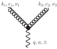
$=\displaystyle\begin{array}[h]{ll}\\ \\ -i{\bm{q}}^{2}\delta^{ac}(n^{\pm})^{\nu},\\ \\ \qquad k^{\pm}=0.\end{array}$ $=\displaystyle\begin{array}[h]{ll}\delta^{ab}\frac{i/2}{{\bm{q}}^{2}}\end{array}$ $\displaystyle=\begin{array}[h]{ll}\\ \\ gf^{c_{1}c_{2}a}\frac{{\bm{q}}^{2}}{k_{1}^{\pm}}(n^{\pm})^{\nu_{1}}(n^{\pm})^{\nu_{2}},\\ \\ \quad k_{1}^{\pm}+k_{2}^{\pm}=0.\end{array}$
(a) (b) (c)

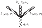
$\displaystyle\begin{array}[h]{l}\displaystyle\\ \displaystyle=ig^{2}{\bm{q}}^{2}\left(\frac{f^{a_{3}a_{2}e}f^{a_{1}ea}}{k_{3}^{\pm}k_{1}^{\pm}}+\frac{f^{a_{3}a_{1}e}f^{a_{2}ea}}{k_{3}^{\pm}k_{2}^{\pm}}\right)(n^{\pm})^{\nu_{1}}(n^{\pm})^{\nu_{2}}(n^{\pm})^{\nu_{3}},\\ \\ \qquad\qquad k_{1}^{\pm}+k_{2}^{\pm}+k_{3}^{\pm}=0.\end{array}$
(d)

Figure 1: Feynman rules for the lowest-order effective vertices of the effective action. Wavy lines denote reggeized fields and curly lines gluons.

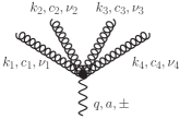
$\begin{array}[h]{ll}\\ =\displaystyle&\displaystyle g^{3}{\bm{q}}^{2}\bigg{[}\frac{f^{c_{4}c_{3}e_{2}}}{k_{4}^{\pm}}\bigg{(}\frac{f^{e_{2}c_{1}e_{1}}f^{c_{2}e_{1}a}}{(k_{1}^{\pm}+k_{2}^{\pm})k_{2}^{\pm}}+\frac{f^{e_{2}c_{2}e_{1}}f^{c_{1}e_{1}a}}{(k_{1}^{\pm}+k_{2}^{\pm})k_{1}^{\pm}}\bigg{)}\\ \\ \displaystyle&\displaystyle+\,\frac{f^{c_{4}c_{1}e_{2}}}{k_{4}^{\pm}}\bigg{(}\frac{f^{e_{2}a_{2}e_{1}}f^{c_{3}e_{1}a}}{(k_{3}^{\pm}+k_{2}^{\pm})k_{3}^{\pm}}+\frac{f^{e_{2}a_{3}e_{1}}f^{c_{2}e_{1}a}}{(k_{3}^{\pm}+k_{2}^{\pm})k_{2}^{\pm}}\bigg{)}\,+\\ \\ \end{array}$
$\begin{array}[h]{l}\displaystyle+\frac{f^{c_{4}c_{2}e_{2}}}{k_{4}^{\pm}}\bigg{(}\frac{f^{e_{2}c_{1}e_{1}}f^{c_{3}e_{1}a}}{(k_{3}^{\pm}+k_{1}^{\pm})k_{3}^{\pm}}+\frac{f^{e_{2}c_{3}e_{1}}f^{c_{1}e_{1}a}}{(k_{3}^{\pm}+k_{1}^{\pm})k_{1}^{\pm}}\bigg{)}\bigg{]}(n^{\pm})^{\nu_{1}}(n^{\pm})^{\nu_{2}}(n^{\pm})^{\nu_{3}}(n^{\pm})^{\nu_{4}},\\ \\ \qquad\qquad\qquad\qquad\qquad\qquad\qquad k_{1}^{\pm}+k_{2}^{\pm}+k_{3}^{\pm}+k_{4}^{\pm}=0.\end{array}$

Figure 2: The order $g^{3}$ induced vertex.

Loop diagrams of the effective action lead to a new type of longitudinal divergences which are not present in conventional quantum corrections to QCD amplitudes, and can be regularized introducing an external parameter $\rho$, evaluated in the limit $\rho\to\infty$, which deforms the light-like vectors $n^{\pm}$ into

$$n^{-} \to n_{a}=e^{-\rho}n^{+}+n^{-},$$

$$n^{+} \to n_{b}=n^{+}+e^{-\rho}n^{-},$$ (6)

without violating the gauge invariance properties of the induced term Eq. (4). While it is possible to identify $\rho$ with a logarithm in $s$ or the rapidity interval spanned by a certain high energy process, we refrain from such an interpretation and consider in the following $\rho$ as an external parameter, similar to the parameter $\epsilon$ in dimensional regularization in $d=4+2\epsilon$ dimensions.

II.2 Pole prescription

The evaluation of loop diagrams requires a prescription to circumvent the light-cone singularities in the induced vertices shown in Figs. 1,2. The seemingly natural choice which is to simply replace the operator $D_{\pm}$ in Eq. (5) by e.g. $D_{\pm}-\epsilon$ does not work in this context as it spoils hermiticity of the effective action. At the level of Feynman diagrams this is reflected by terms that violate high energy factorization. Both effects can be traced back to the existance of new symmetric color tensors, not present in the vertices of Figs. 1, 2. For a more in depth discussion we refer to [23]. This problem can be solved by systematically projecting out these symmetric color structures, order by order in perturbation theory, sticking in this way to the color tensors present in the original vertices Fig. 1, 2. The resulting pole prescription respects then Bose symmetry of the induced vertices and high energy factorization [23]. The $\mathcal{O}(g)$ vertex is taken as a Cauchy principal value:

$$=gf^{c_{1}c_{2}a}\frac{{\bm{q}}^{2}}{[k_{1}^{\pm}]}(n^{\pm})^{\nu_{1}}(n^{\pm})^{\nu_{2}}, \frac{1}{[k_{1}^{\pm}]} \equiv\frac{1}{2}\left(\frac{1}{k_{1}^{\pm}+i\epsilon}+\frac{1}{k_{1}^{\pm}-i\epsilon}\right).$$ (7)

For the $\mathcal{O}(g^{2})$ and $\mathcal{O}(g^{3})$ vertices the light-cone denominators are to be replaced by certain functions $g_{2}$ and $g_{3}$:

$$\parbox{73.97733pt}{\includegraphics[height=56.9055pt]{indu2.pdf}}\begin{array}[h]{l }\\ \displaystyle=-ig^{2}{\bm{q}}^{2}\bigg{[}f^{c_{3}c_{2}e}f^{c_{1}ea}g_{2}^{\pm}(3,2,1)\\ \displaystyle\qquad\qquad\qquad+f^{c_{3}c_{1}e}f^{c_{2}ea}g_{2}^{\pm}(3,1,2)\bigg{]}n^{\pm}_{\nu_{1}}n^{\pm}_{\nu_{2}}n^{\pm}_{\nu_{3}},\end{array}$$ (11)

$$\parbox{85.35826pt}{\includegraphics[height=56.9055pt]{indu3.pdf}}=-g^{3}{\bm{q}}^{2}n^{\pm}_{\nu_{1}}n^{\pm}_{\nu_{2}}n^{\pm}_{\nu_{3}}n^{\pm}_{\nu_{4}}\,\cdot$$

$$\bigg{[} f^{a_{4}a_{1}d_{2}}f^{d_{2}a_{3}d_{1}}f^{d_{1}a_{2}c}g_{3}^{\pm}(4,1,3,2)+f^{a_{4}a_{1}d_{2}}f^{d_{2}a_{2}d_{1}}f^{d_{1}a_{3}c}g_{3}^{\pm}(4,1,2,3)$$

$$+ f^{a_{4}a_{2}d_{2}}f^{d_{2}a_{1}d_{1}}f^{d_{1}a_{3}c}g_{3}^{\pm}(4,2,1,3)+f^{a_{4}a_{2}d_{2}}f^{d_{2}a_{3}d_{1}}f^{d_{1}a_{1}c}g_{3}^{\pm}(4,2,3,1)$$

$$+ f^{a_{4}a_{3}d_{2}}f^{d_{2}a_{1}d_{1}}f^{d_{1}a_{2}c}g_{3}^{\pm}(4,3,1,2)+f^{a_{4}a_{3}d_{2}}f^{d_{2}a_{2}d_{1}}f^{d_{1}a_{1}c}g^{\pm}_{3}(4,3,2,1)\bigg{]}.$$ (12)

They are obtained as

$$g_{2}^{\pm}(i,j,m)=\bigg{[} \frac{-1}{[k_{i}^{\pm}][k_{m}^{\pm}]}-\frac{\pi^{2}}{3}\delta(k_{i}^{\pm})\delta(k_{m}^{\pm})\bigg{]}.$$ (13)

and

$$g_{3}^{\pm}(i,j,m,n)=\bigg{(} \frac{-1}{[k_{i}^{\pm}][k_{n}^{\pm}+k_{m}^{\pm}][k_{n}^{\pm}]}-\frac{\pi^{2}}{3}\delta(k_{n}^{\pm})\delta(k_{m}^{\pm})\frac{-1}{[k_{i}^{\pm}]}$$

$$-\frac{\pi^{2}}{3}\delta(k_{n}^{\pm})\delta(k_{i}^{\pm})\frac{1}{[k_{m}^{\pm}]}-\frac{\pi^{2}}{3}\delta(k_{n}^{\pm}+k_{m}^{\pm})\delta(k_{i}^{\pm})\frac{1}{[k_{n}^{\pm}]}\bigg{)}.$$ (14)

III The gluon Regge trajectory from the effective action

A key ingredient in the resummation of high energy logarithms of QCD scattering amplitudes is provided by a universal function associated with the exchange of a single reggeized gluon, known as the Regge trajectory of the gluon. For the real part of QCD scattering amplitudes, where the high energy description is given in terms of single reggeized gluon exchange, this function is known to govern the entire energy dependence at leading logarithmic (LL) and next-to-leading logarithmic (NLL) accuracy.

Multiple reggeized gluon exchanges appear on the other hand for the high energy description of the imaginary part of scattering amplitudes and in general for amplitudes beyond NLL accuracy. While this requires new elements, which describe in a nutshell the interaction between reggeized gluons, the gluon Regge trajectory remains an essential building block in the formulation of high energy resummation also in this more general case.

To be more precise, for the elastic process $p_{a}+p_{b}\to p_{1}+p_{2}$ with $s=(p_{a}+p_{b})^{2}$ and $t=q^{2}$ with $q=p_{a}-p_{1}$ one finds for amplitudes with gluon quantum numbers in the $t$-channel at LL and NLL accuracy the following factorized form

$$\frac{\mathcal{M}_{(\bf 8_{A})}(s,t)}{\mathcal{M}^{(0)}(s,t)} =\Gamma_{a1}(t)\left[\left(\frac{-s}{-t}\right)^{\omega(t)}+\left(\frac{s}{-t}\right)^{\omega(t)}\right]\Gamma_{b2}(t),$$ (15)

where $\mathcal{M}^{(0)}_{(\bf 8_{A})}$ is the tree-level amplitude and the subscript ‘${\bf 8_{A}}$’ denotes that the allowed $t$-channel exchange is restricted to the anti-symmetric color octet channel. The functions $\Gamma_{ij}(t)$ are known as impact factors, describing the coupling of the reggeized gluons to scattering particles. For the case of gluon and quarks they have been determined within the effective action in [14, 15]. The function $\omega(t)$ which governs the $s$-dependence of the scattering amplitude is on the other hand the Regge trajectory of the gluon. It is currently known to leading [4] and next-leading order [16] for QCD and to all orders in $\mathcal{N}=4$ super Yang-Mills theory [25]. The procedure which allows the derivation of the gluon trajectory from the effective action has been originally discussed in [21]. It consists of two steps

• determination of the propagator of the reggeized gluon to the desired order in $\alpha_{s}$;

• renormalization of the rapidity divergences of the reggeized gluon propagator; the gluon Regge trajectory is then identified as the coefficient of the $\rho$ dependent term in the renormalization factor.

To obtain the reggeized gluon propagator to order $\alpha_{s}^{2}$ it is needed to determine the one- and two-loop self-energies of the reggeized gluon. Following the subtraction procedure proposed in [14] these self-energies can be obtained through

• determination of the self-energy of the reggeized gluon from the effective action, with the reggeized gluon treated as a background field;

• subtraction of all disconnected contributions which contain internal reggeized gluon lines.

Using a symmetric pole prescription as given in Sec. II.2, all diagrams with internal reggeized gluon lines that would possibly contribute to the one loop self energy can be shown to vanish and no subtraction is necessary. The contributing diagrams are shown in Fig. 3.

= + + + + +

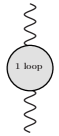
Figure 3: Diagrams contributing to the one-loop reggeized gluon self-energy.

Keeping the ${\cal O}(\rho,\rho^{2})$, for $\rho\to\infty$, terms and using the notation

$$\bar{g}^{2} =\frac{g^{2}N_{c}\Gamma(1-\epsilon)}{(4\pi)^{2+\epsilon}},$$ (16)

we have the following result in $d=4+2\epsilon$ dimensions:

$$\parbox{28.45274pt}{\includegraphics[width=28.45274pt]{self_1loop.pdf}}=\Sigma^{(1)}\left(\rho;\epsilon,\frac{{\bm{q}}^{2}}{\mu^{2}}\right)$$

$$\hskip 11.38092pt=\frac{(-2i{\bm{q}}^{2})\bar{g}^{2}\Gamma^{2}(1+\epsilon)}{\Gamma(1+2\epsilon)}\left(\frac{{\bm{q}}^{2}}{\mu^{2}}\right)^{\epsilon}\bigg{\{}\frac{i\pi-2\rho}{\epsilon}-\frac{1}{(1+2\epsilon)\epsilon}\bigg{[}\frac{5+3\epsilon}{3+2\epsilon}-\frac{n_{f}}{N_{c}}\left(\frac{2+2\epsilon}{3+2\epsilon}\right)\bigg{]}\bigg{\}}.$$ (17)

To determine the 2-loop self energy it is on the other hand needed to subtract disconnected diagrams, whereas diagrams with multiple internal reggeized gluons can be shown to yield a zero result, if the symmetric pole prescription of Sec. II.2 is used. Schematically one has

$$\Sigma^{(2)}\left(\rho;\epsilon,\frac{{\bm{q}}^{2}}{\mu^{2}}\right) =\parbox{56.9055pt}{\centering\includegraphics[height=71.13188pt]{self_2loop.pdf}\@add@centering}=\parbox{56.9055pt}{\centering\includegraphics[height=71.13188pt]{self_2loop_ME.pdf}\@add@centering}-\parbox{56.9055pt}{\centering\includegraphics[height=71.13188pt]{self2_1loop.pdf}\@add@centering},$$ (18)

where the black blob denotes the unsubtracted 2-loop reggeized gluon self-energy, which is obtained through the direct application of the Feynman rules of the effective action, with the reggeized gluon itself treated as a background field. Its determination will be discussed in detail in the forthcoming section. The (bare) two-loop reggeized gluon propagators then reads

$$G\left(\rho;\epsilon,{\bm{q}}^{2},\mu^{2}\right) =\frac{i/2}{{\bm{q}}^{2}}\left\{1+\frac{i/2}{{\bm{q}}^{2}}\Sigma\left(\rho;\epsilon,\frac{{\bm{q}}^{2}}{\mu^{2}}\right)+\left[\frac{i/2}{{\bm{q}}^{2}}\Sigma\left(\rho;\epsilon,\frac{{\bm{q}}^{2}}{\mu^{2}}\right)\right]^{2}+\ldots\right\},$$ (19)

with

$$\Sigma\left(\rho;\epsilon,\frac{{\bm{q}}^{2}}{\mu^{2}}\right) =\Sigma^{(1)}\left(\rho;\epsilon,\frac{{\bm{q}}^{2}}{\mu^{2}}\right)+\Sigma^{(2)}\left(\rho;\epsilon,\frac{{\bm{q}}^{2}}{\mu^{2}}\right)+\ldots$$ (20)

where the dots indicate higher order terms. As discussed in Sec. II.1 and as directly apparent from Eq. (III), the reggeized gluon self-energies are divergent in the limit $\rho\to\infty$. In [14, 15] it has been demonstrated by explicit calculations that these divergences cancel at one-loop level, for both quark-quark and gluon-gluon scattering amplitudes, against divergences in the couplings of the reggeized gluon to external particles. The entire one-loop amplitude is then found to be free of any high energy singularity in $\rho$. High energy factorization then suggests that such a cancellation holds also beyond one loop. Starting from this assumption, it is possible to define a renormalized reggeized gluon propagator through

$$G^{\rm R}(M^{+},M^{-};\epsilon,\bm{q}^{2},\mu^{2})=\frac{G(\rho;\epsilon,\bm{q}^{2},\mu^{2})}{Z^{+}\left(\frac{M^{+}}{\sqrt{\bm{q}^{2}}},\rho;\epsilon,\frac{\bm{q}^{2}}{\mu^{2}}\right)Z^{-}\left(\frac{M^{-}}{\sqrt{\bm{q}^{2}}},\rho;\epsilon,\frac{\bm{q}^{2}}{\mu^{2}}\right)},$$ (21)

where the renormalization factors need to cancel against corresponding renormalization factors associated with the vertex to which the reggeized gluon couples with ‘plus’ ($Z^{+}$) and ‘minus’ ($Z^{-}$) polarization. For explicit examples we refer the reader to [15, 21]. In their most general form these renormalization factors are parametrized as

$$Z^{\pm}\left(\frac{M^{\pm}}{\sqrt{\bm{q}^{2}}},\rho;\epsilon,\frac{\bm{q}^{2}}{\mu^{2}}\right)=\exp\left[\left(\frac{\rho}{2}-\ln\frac{M^{\pm}}{\sqrt{\bm{q}^{2}}}\right)\omega\left(\epsilon,\frac{\bm{q}^{2}}{\mu^{2}}\right)+f^{\pm}\left(\epsilon,\frac{\bm{q}^{2}}{\mu^{2}}\right)\right],$$ (22)

with the coefficient of the $\rho$-divergent term given by the gluon Regge trajectory $\omega(\epsilon,{\bm{q}}^{2})$. It is assumed to have the following perturbative expansion

$$\omega\left(\epsilon,\frac{{\bm{q}}^{2}}{\mu^{2}}\right) =\omega^{(1)}\left(\epsilon,\frac{{\bm{q}}^{2}}{\mu^{2}}\right)+\omega^{(2)}\left(\epsilon,\frac{{\bm{q}}^{2}}{\mu^{2}}\right)+\ldots,$$ (23)

and is to be determined by the requirement that the renormalized reggeized gluon propagator must, at each loop order, be free of $\rho$ divergences. At one loop we get from Eq. (III)

$$\omega^{(1)}\left(\epsilon,\frac{{\bm{q}}^{2}}{\mu^{2}}\right) =-\frac{2\bar{g}^{2}\Gamma^{2}(1+\epsilon)}{\Gamma(1+2\epsilon)\epsilon}\left(\frac{{\bm{q}}^{2}}{\mu^{2}}\right)^{\epsilon}.$$ (24)

The function $f^{\pm}(\epsilon,{\bm{q}}^{2})$ parametrizes finite contributions and is, in principle, arbitrary. While symmetry of the scattering amplitude requires $f^{+}=f^{-}=f$, Regge theory suggests fixing it in such a way that terms which are not enhanced in $\rho$ are entirely transferred from the reggeized gluon propagators to the vertices, to which the reggeized gluon couples. With the perturbative expansion

$$f\left(\epsilon,\frac{{\bm{q}}^{2}}{\mu^{2}}\right) =f^{(1)}\left(\epsilon,\frac{{\bm{q}}^{2}}{\mu^{2}}\right)+f^{(2)}\left(\epsilon,\frac{{\bm{q}}^{2}}{\mu^{2}}\right)\ldots$$ (25)

we obtain from Eq. (III)

$$f^{(1)}\left(\epsilon,\frac{{\bm{q}}^{2}}{\mu^{2}}\right) =\frac{\bar{g}^{2}\Gamma^{2}(1+\epsilon)}{\Gamma(1+2\epsilon)}\left(\frac{{\bm{q}}^{2}}{\mu^{2}}\right)^{\epsilon}\frac{(-1)}{(1+2\epsilon)2\epsilon}\bigg{[}\frac{5+3\epsilon}{3+2\epsilon}-\frac{n_{f}}{N_{c}}\left(\frac{2+2\epsilon}{3+2\epsilon}\right)\bigg{]}.$$ (26)

The renormalized reggeized gluon propagator is then to one loop accuracy given by

$$G^{\rm R}(M^{+},M^{-};\epsilon,\bm{q}^{2},\mu^{2}) =1+\omega^{(1)}\left(\epsilon,\frac{{\bm{q}}^{2}}{\mu^{2}}\right)\left(\log\frac{M^{+}M^{-}}{{\bm{q}}^{2}}-\frac{i\pi}{2}\right)+\ldots$$ (27)

The scales $M^{+}$ and $M^{-}$ are arbitrary; their role is analogous to the renormalization scale in UV renormalization and the factorization scale in collinear factorization. They are naturally chosen to coincide with the corresponding light-cone momenta of scattering particles to which the reggeized gluon couples. To determine the gluon Regge trajectory at two loops we need in addition the $\rho$-enhanced terms of the two-loop reggeized gluon self-energy. From Eq. (27) we obtain the following relation

$$\omega^{(2)}\left(\epsilon,\frac{{\bm{q}}^{2}}{\mu^{2}}\right) =\lim_{\rho\to\infty}\frac{1}{\rho}\bigg{[}\frac{\Sigma^{(2)}}{(-2i{\bm{q}}^{2})}+\left(\frac{\Sigma^{(1)}}{(-2i{\bm{q}}^{2})}\right)^{2}-\left(\rho\omega^{(1)}+2f^{(1)}\right)\frac{\Sigma^{(1)}}{(-2i{\bm{q}}^{2})}$$

$$\qquad\qquad\qquad\qquad\qquad\qquad\qquad\qquad+\frac{\rho^{2}}{2}\left(\omega^{(1)}\right)^{2}+2\rho f^{(1)}\omega^{(1)}\bigg{]}$$

$$=\lim_{\rho\to\infty}\frac{1}{\rho}\bigg{[}\frac{\Sigma^{(2)}}{(-2i{\bm{q}}^{2})}+\frac{\rho^{2}}{2}\left(\omega^{(1)}\right)^{2}+2\rho f^{(1)}\omega^{(1)}\bigg{]},$$ (28)

where we omitted at the right hand side the dependencies on $\epsilon$ and ${\bm{q}}^{2}/\mu^{2}$; in the last line we further expanded $\Sigma^{(1)}$ in terms of the functions $\omega^{(1)}$ and $f^{(1)}$. We stress that this is a non-trivial definition and that it is not clear a priori whether the right hand side even exists due to the presence of the second term, linear in $\rho$. Confirmation of this relation provides therefore an important non-trivial check on the validity of our formalism.

IV Computation of the 2-Loop reggeized gluon self-energy

The necessary diagrams for the computation of the unsubtracted reggeized gluon self-energy are shown in Fig. 4.

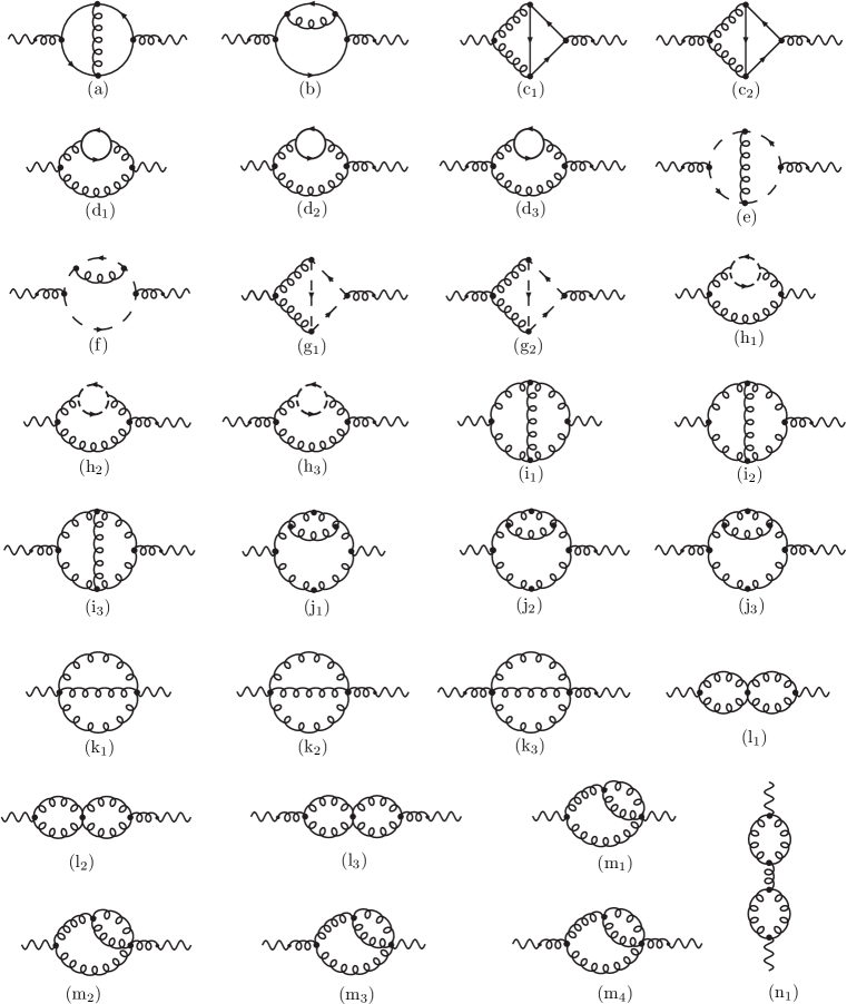
Figure 4: Diagrams for the two-loop trajectory in the effective action formalism. Tadpole-like contributions are zero in dimensional regularization and are omitted.

The diagrams (a₁)-(d₃), containing internal quark loops, generating an overall factor $n_{f}$, have been computed in [21] and lead to the following result,

$$=-\rho(-i2{\bm{q}}^{2})\bar{g}^{4}\frac{4n_{f}}{\epsilon N_{c}}\frac{\Gamma^{2}(2+\epsilon)}{\Gamma(4+2\epsilon)}\cdot\frac{3\Gamma(1-2\epsilon)\Gamma(1+\epsilon)\Gamma(1+2\epsilon)}{\Gamma^{2}(1-\epsilon)\Gamma(1+3\epsilon)\epsilon}+\mathcal{O}(\rho^{0})\,.$$ (29)

IV.1 The scaling argument

For the computation of the remaining diagrams we observe at first that the number of diagrams, which can be potentially enhanced by a factor $\rho^{k}$, $k\geq 1$, is largely reduced by scaling arguments: only those diagrams where both reggeized gluons couple to the internal gluon lines through induced reggeized gluon–$n$-gluon vertices with $n\geq 2$ have the potential to lead to an enhancement through a factor $\rho$. This is immediately clear for diagrams where both reggeized gluons couple through the reggeized gluon–$1$-gluon vertex Fig. 1 (a) to the internal QCD lines. Those diagrams are a projection of the 2-loop QCD polarization tensor onto the kinematics of reggeized gluons and no $\rho$ enhancement can be expected.

To address the case where only one of the reggeized gluons couples through an induced reggeized gluon–$n$-gluon ($n\geq 2$) vertex to the internal QCD particles, we consider the general diagram in Fig. 5.

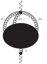
Figure 5: General non-enhanced diagram.

The dependence on the light-cone vectors of the reggeized gluon–$n$-gluon vertex in Fig. 5 is, up to permutations, of the form $\frac{n_{a}^{\mu_{1}}n_{a}^{\mu_{2}}\cdots n_{a}^{\mu_{d}}}{n_{a}\cdot k_{1}n_{a}\cdot k_{2}\cdots n_{a}\cdot k_{n-1}}$. The denominators $n_{a}\cdot k_{i}$, $i=1,\ldots n-1$ appear in the integrals that give rise to an amplitude ${\cal M}_{\mu_{1}\mu_{2}\cdots\mu_{n}\nu}$. In a general diagram such as Fig. 5, the only vectors that are not integrated over in the amplitude are $q$, the momentum transfer, and $n_{a}$, which enters through the denominators of the induced vertex. The vector $n_{b}$ only contracts with the four-vector index $\nu$. The whole diagram can be therefore written as

$$n_{a}^{\mu_{1}}n_{a}^{\mu_{2}}\cdots n_{a}^{\mu_{n}}{\cal M}_{\mu_{1}\mu_{2}\cdots\mu_{n}\nu}(n_{a},q)n_{b}^{\nu}.$$ (30)

As a consequence, the tensor structure of ${\cal M}_{\mu_{1}\mu_{2}\cdots\mu_{n}\nu}(n_{a},q)$ can only consist of combinations of the four vector $n_{a}^{\mu}$ and the metric tensor $g_{\mu\nu}$, since the external reggeized gluons imply $q\cdot n_{a}=q\cdot n_{b}=0$. The only scalar combinations that can appear are therefore $\bm{q}^{2}$ and $n_{a}^{2}$. These factors must give the dimensions required by scale transformations. If $s$ is the number of metric tensors in the numerator for a given term and $l$ the number of $n_{a}^{\mu}$ numerators, then $n+1=2s+l$ and the associated scalar function must scale as

$$\frac{1}{n_{a}^{n-1+l}}=\frac{1}{(n_{a}^{2})^{d-s}}.$$ (31)

Next, we consider the contractions with the vertex currents. If $n_{b}^{\rho}$ is contracted through a metric tensor then we obtain

$$(n_{a}^{2})^{l}\,n_{a}\cdot n_{b}\,(n_{a}^{2})^{s-1} =(n_{a}^{2})^{n-s}n_{a}\cdot n_{b};$$ (32)

if on the other hand $n_{b}^{\rho}$ is directly contracted with one of the $n_{a}$’s, we obtain a factor

$$n_{a}\cdot n_{b}\,(n_{a}^{2})^{s}(n_{a}^{2})^{l-1} =(n_{a}^{2})^{n-s}n_{a}\cdot n_{b}.$$ (33)

In both cases the factors of $n_{a}^{2}$ cancel against corresponding factors in the denominators and no enhancement can occur. Thus, in our case only the diagrams (h₁), (i₁), (j₁), (k₁), (l₁), (m₁) and (n₁) are potentially enhanced by (powers of) $\rho$.

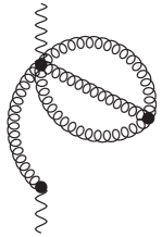
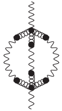
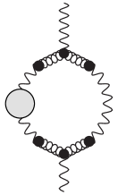
(a)

(b)

Figure 6: (a) typical tadpole contribution to the 2-loop self energy (b) disconnected diagrams with internal reggeized gluon loops which would contribute to possible subtraction terms. Both contributions can be shown to vanish.

A further class of diagrams that can be omitted are tadpole diagrams and diagrams with internal reggeized gluon loops. Tadpole diagrams, such as in Fig. 6 (a), have been verified to vanish in dimensional regularization. Possible loop diagrams with internal reggeized gluon lines, such as Fig. 6 (b) vanish identically due to the symmetry properties obeyed by the pole prescription of the induced vertices.

IV.2 Calculation of the enhanced diagrams

Direct computation reveals that diagram (l₁) is identically zero. We use the notation $\xi=n_{a}^{2}=n_{b}^{2}=4e^{-\rho}$, $\delta=n_{a}\cdot n_{b}\sim 2$, and the following shorthand notation for the master integral

$$[\,\alpha_{1},\alpha_{2},\cdots,\alpha_{9}\,]=(\mu^{4})^{4-d}\iint\frac{d^{d}k}{(2\pi)^{d}}\frac{d^{d}l}{(2\pi)^{d}}\frac{1}{(-k^{2}-i0)^{\alpha_{1}}[-(k-q)^{2}-i0]^{\alpha_{2}}(-l^{2}-i0)^{\alpha_{3}}}$$

$$\times\frac{1}{[-(l-q)^{2}-i0]^{\alpha_{4}}[-(k-l)^{2}-i0]^{\alpha_{5}}}\cdot\frac{1}{(-n_{a}\cdot k)^{\alpha_{6}}(-n_{b}\cdot k)^{\alpha_{7}}(-n_{a}\cdot l)^{\alpha_{8}}(-n_{b}\cdot l)^{\alpha_{9}}},$$ (34)

with $n_{a}\cdot q=n_{b}\cdot q=0$ and the eikonal factors taken with the pole prescription defined in Sec. II.2. More accurately, for master integrals with single poles $1/n_{a,b}\cdot k$ ($\alpha_{6}=1,\alpha_{8}=0$, $\alpha_{6}=0,\alpha_{8}=1$ and/or $\alpha_{7}=1,\alpha_{9}=0$, $\alpha_{7}=0,\alpha_{9}=1$) the function $g_{1}^{a,b}$ is used, while for terms with two poles $1/n_{a,b}\cdot k/n_{a,b}\cdot l$ ($\alpha_{6}=1,\alpha_{8}=1$, and/or $\alpha_{7}=1,\alpha_{9}=1$) the function $g_{2}^{a,b}$ is employed. Dropping all pieces that cannot generate terms enhanced as $\rho\to\infty$, we have the following contributions from each diagram:

$$\left[i{\cal M}_{\rm h_{1}}\right]_{\rm enh} =-\frac{3ig^{4}}{4(3+2\epsilon)S_{\rm h_{1}}}\delta^{2}\bm{q}^{2}N_{c}^{2}{[1,0,0,1,1,0,0,1,1]};\quad S_{\rm h_{1}}=1.$$ (35)

$$\left[i{\cal M}_{\rm i_{1}}\right]_{\rm enh} =\frac{ig^{4}}{2S_{\rm i_{1}}}(\bm{q}^{2})^{2}N_{c}^{2}\bigg{[}\delta^{2}\bigg{\{}2\bm{q}^{2}{[1,1,1,1,1,1,0,0,1]}+{[1,1,1,1,0,1,0,0,1]}$$

$$-4{[1,1,1,0,1,1,0,0,1]}\bigg{\}}+8\xi{[1,1,1,1,1,1,-2,0,1]}\bigg{]};\quad S_{\rm i_{1}}=2.$$

$$\left[i{\cal M}_{\rm j_{1}}\right]_{\rm enh} =-\frac{3ig^{4}}{2S_{\rm j_{1}}}\bm{q}^{2}N_{c}^{2}\delta^{2}\frac{19+12\epsilon}{3+2\epsilon}{[1,0,0,1,1,0,0,1,1]};\quad S_{\rm j_{1}}=2.$$

$$\left[i{\cal M}_{\rm k_{1}}\right]_{\rm enh} =\frac{3ig^{4}}{2S_{\rm k_{1}}}(\bm{q}^{2})^{2}N_{c}^{2}\delta^{3}{[1,0,0,1,1,1,1,1,1]};\quad S_{\rm k_{1}}=6.$$

$$\left[i{\cal M}_{\rm m_{1}}\right]_{\rm enh} =\frac{ig^{4}}{S_{\rm m_{1}}}(\bm{q}^{2})^{2}N_{c}^{2}\delta\bigg{[}-\frac{6\delta}{\bm{q}^{2}}{[1,0,0,1,1,0,0,1,1]}+2{[1,1,1,0,1,1,0,0,1]}$$

$$+2\xi{[1,1,0,1,1,1,1,-1,1]}\bigg{]};\quad S_{\rm m_{1}}=1.$$

$$\left[i{\cal M}_{\rm n_{1}}\right]_{\rm enh} =0.$$

In some cases, we have used the Mathematica package FIRE [26] that implements the Laporta algorithm [27] to reduce the number and complexity of master integrals through integration-by-parts identities [28]. Discarding all contributions which are finite or suppressed in the limit $\rho\to\infty$, we can express the entire unsubtracted two-loop self-energy in terms of 7 master integrals $\mathcal{A}-\mathcal{G}$ with a certain coefficient associated with each master integral, see Tab. 1.

$$\begin{array}[h]{rcl|c}&&\text{master integral}&\text{coefficent}\\ \hline\cr{\cal A}&\equiv&\big{[}1,1,1,1,0,1,0,0,1\big{]}&\displaystyle c_{\mathcal{A}}=-\frac{\bm{q}^{2}}{2}\\ {\cal B}&\equiv&\big{[}1,0,0,1,1,0,0,1,1\big{]}&\displaystyle c_{\mathcal{B}}=\frac{66+42\epsilon}{3+2\epsilon}\\ {\cal C}&\equiv&\big{[}1,1,1,1,1,1,0,0,1\big{]}&\displaystyle c_{\mathcal{C}}=-(\bm{q}^{2})^{2}\\ \displaystyle{\cal D}&\equiv&[1,0,0,1,1,1,1,1,1\big{]}&c_{\mathcal{D}}=-\bm{q}^{2}\\ {\cal E}&\equiv&\big{[}1,1,0,1,1,1,1,-1,1\big{]}&c_{\mathcal{E}}=-2{\xi}\bm{q}^{2}\\ {\cal F}&\equiv&\big{[}1,1,1,1,1,1,-2,0,1\big{]}&\displaystyle c_{\mathcal{F}=}-{\xi}\bm{q}^{2}\\ {\cal G}&\equiv&\big{[}1,1,1,0,1,1,0,0,1\big{]}&\displaystyle c_{\mathcal{G}}=0\\ \end{array}$$

Table 1: Coefficients of the master integrals. Each coefficient is in addition to be multiplied with the common overall factor $(-2i\bm{q}^{2})g^{4}N_{c}^{2}$.

The master integral ${\cal A}$ can be shown to vanish by symmetry due to the symmetric pole prescription of the eikonal poles of the induced vertices. The $\rho$-enhanced pieces of the remaining master integrals are computed up to terms of order ${\cal O}(\epsilon)$ using the Mellin-Barnes representations technique, for a review see e.g. [29].

To this end, we first derive multi-contour integral representations for the master integrals, referring the reader for details to Appendix A.1. Having as working environment the code MB.m [30], we use the Mathematica package MBasymptotics.m [32] to perform an asymptotic expansion in $e^{-\rho}$. We remove any terms proportional to $e^{-k\rho\epsilon},\,k\in\mathbbm{Z}$, capturing this way the leading behavior in $\rho$. As a final step, we resolve the singularities structure in $\epsilon$ by using the Mathematica packages MB.m and MBresolve.m. Eventually, some of the final integrals are further simplified by using the Barnes’ lemmas implemented in the Mathematica code barnesroutines.m [33].

Following this procedure we obtain for the master integrals the following results:

$$c_{\mathcal{B}}\cdot{\cal B} =\frac{1}{(4\pi)^{4}}\left[\frac{11}{\epsilon^{2}}-\frac{1+66\Xi}{3\epsilon}+\frac{400+12\Xi+396\Xi^{2}-33\pi^{2}}{18}\right]\rho,$$

$$c_{\mathcal{C}}\cdot{\cal C} =\frac{1}{(4\pi)^{4}}\bigg{(}\bigg{[}-\frac{4}{\epsilon^{3}}-\frac{8(1-\Xi)}{\epsilon^{2}}-\frac{\pi^{2}+8(1-\Xi)^{2}}{\epsilon}-2\pi^{2}(1-\Xi)-\frac{16(1-\Xi)^{3}}{3}$$

$$-\frac{50}{3}\zeta(3)\bigg{]}\rho+\left[\frac{2}{\epsilon^{2}}+\frac{4(1-\Xi)}{\epsilon}+\frac{1}{3}(12(1-\Xi)^{2}-\pi^{2})\right]\left\{\rho^{2}-i\pi\rho\right\}\bigg{)},$$

$$c_{\mathcal{D}}\cdot{\cal D} =\frac{1}{(4\pi)^{4}}\bigg{[}\frac{4}{\epsilon^{3}}+\frac{8(1-\Xi)}{\epsilon^{2}}+\frac{4(\pi^{2}+6(1-\Xi)^{2})}{3\epsilon}+\frac{8\pi^{2}(1-\Xi)}{3}$$

$$+\frac{16(1-\Xi)^{3}}{3}+\frac{44\zeta(3)}{3}\bigg{]},$$

$$c_{\mathcal{E}}\cdot{\cal E} =0,$$

$$c_{\mathcal{F}}\cdot{\cal F} =\frac{1}{(4\pi)^{4}}\left[-\frac{4}{\epsilon^{2}}+\frac{8\Xi}{\epsilon}+\frac{2\pi^{2}}{3}-8(1+\Xi^{2})\right],$$ (36)

where we introduced the notation

$$\Xi =1-\gamma_{E}-\ln\frac{\bm{q}^{2}}{4\pi\mu^{2}}.$$ (37)

Using these results, the (unsubtracted) contribution to the reggeized gluon self-energy (with $n_{f}=0$) reads:

$$=\begin{array}[h]{l}\displaystyle(-2i{\bm{q}}^{2})\frac{g^{4}N_{c}^{2}}{(4\pi)^{4}}\Bigg{(}\left\{\frac{2}{\epsilon^{2}}+\frac{4(1-\Xi)}{\epsilon}+4(1-\Xi)^{2}-\frac{\pi^{2}}{3}\right\}\rho^{2}+\bigg{\{}\frac{7}{\epsilon^{2}}-\frac{14\Xi}{\epsilon}\\ \vspace{.cm}\displaystyle\qquad\qquad-\frac{1-\pi^{2}}{3\epsilon}-2\frac{\Xi(\pi^{2}-1)}{3}+14(1+\Xi^{2})+\frac{2}{9}-\frac{\pi^{2}}{2}-2\zeta(3)\\ \displaystyle\qquad\qquad\qquad-i\pi\left[\frac{2}{\epsilon^{2}}+4\frac{1-\Xi}{\epsilon}+\frac{1}{3}(12(1-\Xi)^{2}-\pi^{2})\right]\bigg{\}}\rho\Bigg{)}\,.\end{array}$$ (41)

Expanding in $\epsilon$ the expression in Eq. (18), one eventually finds for the subtracted reggeized gluon self-energy for $n_{f}=0$:

$$\Sigma^{(2)}_{{n_{f}=0}}\left(\rho,\frac{\bm{q}^{2}}{\mu^{2}}\right) =\parbox{28.45274pt}{ \includegraphics[height=56.9055pt]{self_2loop.pdf}}=\parbox{28.45274pt}{ \includegraphics[height=56.9055pt]{self_2loop_ME.pdf}}-\parbox{28.45274pt}{ \includegraphics[height=56.9055pt]{self2_1loop.pdf}}=(-2i{\bm{q}}^{2})\frac{g^{4}N_{c}^{2}}{(4\pi)^{4}}\bigg{\{}-\bigg{[}\frac{2}{\epsilon^{2}}+\frac{4(1-\Xi)}{\epsilon}$$

$$+4(1-\Xi)^{2}-\frac{\pi^{2}}{3}\bigg{]}\rho^{2}+\bigg{[}\frac{1}{3\epsilon^{2}}+\frac{1}{9\epsilon}+\frac{\pi^{2}}{3\epsilon}-\frac{2\Xi}{3\epsilon}+\frac{\pi^{2}(11-12\Xi)}{18}$$

$$+\frac{16}{27}-\frac{2}{9}\Xi+\frac{2}{3}\Xi^{2}-2\zeta(3)\bigg{)}\bigg{]}\rho\bigg{\}}+\mathcal{O}(\epsilon)+\mathcal{O}(\rho^{0}).$$ (42)

Now we can compare our result for the 2-loop self-energy with the definition of the 2-loop gluon Regge trajectory, Eq. (III). At first we note that all divergent terms $\sim\rho$ cancel against each other since the terms quadratic in $\rho$ in Eq. (IV.2) cancel precisely the term $[\rho\omega^{(1)}]^{2}/2$ in Eq. (III), i.e.

$$(\omega^{(1)})^{2}\frac{\rho^{2}}{2}+\frac{\Sigma_{\rho^{2}}^{(2)}}{(-2i\bm{q}^{2})} =0,$$ (43)

if the first term is expanded up to $\mathcal{O}(\epsilon)$. Taking the function $f^{(1)}$ in the limit $n_{f}=0$, the remaining terms then yield the 2-loop Regge gluon trajectory for zero flavors,

$$\omega^{(2)}(\bm{q}^{2})|_{n_{f}=0}=\frac{(\omega^{(1)}(\bm{q}^{2}))^{2}}{4}\left[\frac{11}{3}+\left(\frac{\pi^{2}}{3}-\frac{67}{9}\right)\epsilon+\left(\frac{404}{27}-2\zeta(3)\right)\epsilon^{2}\right],$$ (44)

which is in complete agreement with the results in the literature [16]. The terms proportional to $n_{f}$ have been calculated in [21]. With the the flavor-dependent $\rho$-enhanced terms, the subtracted 2-loop self-energy is given by

$$\Sigma^{(2)}_{n_{f}}\left(\rho;\epsilon,\frac{{\bm{q}}^{2}}{\mu^{2}}\right) =\frac{\rho(-2i{\bm{q}}^{2})\bar{g}^{4}4n_{f}}{\epsilon N_{c}}\frac{\Gamma^{2}(2+\epsilon)}{\Gamma(4+2\epsilon)}\left(\frac{{\bm{q}}^{2}}{\mu^{2}}\right)^{2\epsilon}\bigg{(}\frac{\Gamma^{2}(1+\epsilon)}{\Gamma(1+2\epsilon)}\frac{4}{\epsilon}$$

$$\quad\qquad\qquad\quad\qquad\qquad\qquad\qquad-\frac{3\Gamma(1-2\epsilon)\Gamma(1+\epsilon)\Gamma(1+2\epsilon)}{\Gamma^{2}(1-\epsilon)\Gamma(1+3\epsilon)\epsilon}\bigg{)},$$ (45)

and one obtains for the 2-loop Regge gluon trajectory with $n_{f}$ flavors

$$\omega^{(2)}(\bm{q}^{2})=\frac{(\omega^{(1)}(\bm{q}^{2}))^{2}}{4}\left[\frac{11}{3}-\frac{2n_{f}}{3N_{c}}+\left(\frac{\pi^{2}}{3}-\frac{67}{9}\right)\epsilon+\left(\frac{404}{27}-2\zeta(3)\right)\epsilon^{2}\right].$$ (46)

V Conclusions and Outlook

In this paper we have presented a derivation of the two-loop gluon Regge trajectory using Lipatov’s effective action and a recently developed computational scheme, which includes a regularization, subtraction and renormalization procedure. Our result is in precise agreement with earlier results present in the literature and thus provides a highly non-trivial check of the effective action and our proposed computational framework.

From a technical point of view, the main result of the paper is the computation of the 2-loop reggeized gluon self-energy. Regularizing high energy divergences by slightly moving the light-like vectors of the effective action away from the light-cone, we first demonstrated the suppression of a large class of diagrams through a scaling argument. The remaining diagrams were then expressed in terms of seven master integrals, which have been evaluated using multiple Mellin-Barnes representations. Our scheme introduces a consistent general strategy to deal with more complex computations, with the hope to easy the path to perform further calculations with Lipatov’s high-energy effective action.

Appendix A Appendix

In this appendix we present some details of the derivation of Mellin-Barnes representations for the general two-loop master integral considered in this work with propagators to arbitrary powers. The principal tool in this analysis is the formula

$$\frac{1}{(X_{1}+\cdots+X_{n})^{\lambda}} =\frac{1}{\Gamma(\lambda)}\frac{1}{(2\pi i)^{n-1}}\int\cdots\int_{-i\infty}^{+i\infty}dz_{2}\cdots dz_{n}\prod_{i=2}^{n}X_{i}^{z_{i}}X_{1}^{-\lambda-z_{2}-\cdots-z_{n}}$$ (47)

$$\times\Gamma(\lambda+z_{2}+\cdots+z_{n})\prod_{i=2}^{n}\Gamma(-z_{i}),$$

where the contours of integration are such that poles with a $\Gamma(\cdots+z_{i})$ dependence are to the left of the $z_{i}$ contour and poles with a $\Gamma(\cdots-z_{i})$ dependencies lie to the right of the $z_{i}$ contour.

A.1 Mellin-Barnes Representation for Master Integrals without phases

We consider the integral

$$\mathcal{S}_{1}=\int\frac{d^{d}k}{(2\pi)^{d}} \frac{1}{(-k^{2}-i0)^{C}[-(k-q)^{2}-i0]^{D}[-(k-l)^{2}-i0]^{E}}$$

$$\times\frac{1}{(-n_{a}\cdot k-i0)^{\mu_{1}}(-n_{b}\cdot k-i0)^{\mu_{2}}},$$ (48)

where the relation $n_{a}\cdot q=n_{b}\cdot q=0$ is implied. Unlike the general master integral defined in Eq. (IV.2), the contour of integration is in the following always defined to lie above the singularities introduced by the light cone denominators. The treatment of alternating descriptions, contained in the functions $g_{1}$ and $g_{2}$ is summarized in Appendix A.2.

Using Schwinger parameters, we can write

$$\mathcal{S}_{1} =\frac{i^{C+D+E+\mu_{1}+\mu_{2}}}{\Gamma(C)\Gamma(D)\Gamma(E)\Gamma(\mu_{1})\Gamma(\mu_{2})}\int_{0}^{\infty}\cdots\int_{0}^{\infty}d\alpha d\beta d\gamma d\tilde{\delta}d\tilde{\sigma}\,$$ (49)

$$\hskip 113.81102pt\alpha^{C-1}\beta^{D-1}\gamma^{E-1}\tilde{\delta}^{\mu_{1}-1}\tilde{\sigma}^{\mu_{2}-1}\int\frac{d^{d}k}{(2\pi)^{d}}e^{i{\cal D}},$$

$${\cal D}=\alpha k^{2}+\beta(k-q)^{2}+\gamma(k-l)^{2}+\tilde{\delta}n_{a}\cdot k+\tilde{\sigma}n_{b}\cdot k$$

$$\qquad\qquad=(\alpha+\beta+\gamma)k^{2}+\beta q^{2}+\gamma l^{2}-2k\cdot\left(\beta q+\gamma l-\left[\tilde{\delta}\frac{n_{a}}{2}+\tilde{\sigma}\frac{n_{b}}{2}\right]\right).$$

With a shift in the momentum integral and introducing parameters $\lambda=\alpha+\beta+\gamma,\,\xi=\frac{\beta}{\alpha+\beta},\,\eta=\frac{\gamma}{\alpha+\beta+\gamma};\,\,\tilde{\delta}=2\lambda\delta,\,\tilde{\sigma}=2\lambda\sigma,$ and $x=2(\delta+\sigma),\,y=\frac{\delta}{\delta+\sigma}$, we arrive at

$$\mathcal{S}_{1}= \frac{i^{C+D+E+\mu_{1}+\mu_{2}}}{\Gamma(C)\Gamma(D)\Gamma(E)\Gamma(\mu_{1})\Gamma(\mu_{2})}\int_{0}^{\infty}d\lambda\,\lambda^{C+D+E+\mu_{1}+\mu_{2}-1}\int_{0}^{\infty}dx\,x^{\mu_{1}+\mu_{2}-1}$$

$$\int_{0}^{1}d\xi\,\xi^{D-1}(1-\xi)^{C-1}\int_{0}^{1}d\eta\,\eta^{E-1}(1-\eta)^{C+D-1}\int_{0}^{1}dyy^{\mu_{1}-1}(1-y)^{\mu_{2}-1}\int\frac{d^{d}k}{(2\pi)^{d}}$$

$$\exp\left[i\lambda\big{(}k^{2}-(1-\eta)^{2}\xi(1-\xi)\bm{q}^{2}-\eta(1-\eta)(1-\xi)(-l^{2})-\eta(1-\eta)\xi[-(l-q)^{2}]\right.$$

$$\left.-\eta x[y(-n_{a}\cdot l)+(1-y)(-n_{b}\cdot l)-x^{2}(\Psi y(1-y)+e^{-\rho})\big{)}\right],$$ (50)

where $\Psi\equiv(1-e^{-\rho})^{2}$. Performing the integration over momentum and the parameter $\lambda$ we obtain with Eq. (47)

$$\mathcal{S}_{1} =\frac{i}{(4\pi)^{d/2}\Gamma(C)\Gamma(D)\Gamma(E)\Gamma(\mu_{1})\Gamma(\mu_{2})}\int_{0}^{1}d\xi\,\xi^{D-1}(1-\xi)^{C-1}\int_{0}^{1}d\eta\,\eta^{E-1}(1-\eta)^{C+D-1}$$ (51)

$$\int_{0}^{\infty}dx\,x^{\mu_{1}+\mu_{2}-1}\int_{0}^{1}dy\,y^{\mu_{1}-1}(1-y)^{\mu_{2}-1}\,\int\cdots\int_{-i\infty}^{+i\infty}\frac{dz_{2}}{2\pi i}\cdots\frac{dz_{7}}{2\pi i}\Gamma(-z_{2})\cdots\Gamma(-z_{7})$$

$$\Gamma(z_{2}+z_{3}+z_{4}+z_{5}+z_{6}+z_{7}+C+D+E+\mu_{1}+\mu_{2}-d/2)[(1-\eta)^{2}\xi(1-\xi)\bm{q}^{2}]^{z_{2}}$$

$$\frac{[\eta(1-\eta)(1-\xi)(-l^{2})]^{z_{3}}[\eta(1-\eta)\xi(-(l-q)^{2})]^{z_{4}}[\eta xy(-a\cdot l)]^{z_{5}}[\eta x(1-y)(-b\cdot l)]^{z_{6}}}{[x^{2}y(1-y)]^{z_{2}+z_{3}+z_{4}+z_{5}+z_{6}+z_{7}+C+D+E+\mu_{1}+\mu_{2}-d/2}[x^{2}(e^{-\rho})]^{-z_{7}}},$$

which allows to perform the integrations over the parameters $\xi,\eta,x$ and $y$. In some cases integrals of the form

$$\int_{0}^{1}dy\,y^{\alpha-1}(1-y)^{-\alpha-1}=\int_{0}^{\infty}dt\,t^{-\alpha-1}=2\pi i\delta\left(\alpha\right)$$ (52)

appear which allow for the reduction of contour integrals. Eventually, we arrive at

$$\mathcal{S}_{1} =\frac{i}{(4\pi)^{d/2}}\int\cdots\int\frac{dz_{2}}{2\pi i}\frac{dz_{3}}{2\pi i}\frac{dz_{4}}{2\pi i}\frac{dz_{5}}{2\pi i}\frac{dz_{7}}{2\pi i}\frac{\Gamma(-z_{2})\Gamma(-z_{3})\Gamma(-z_{4})\Gamma(-z_{5})\Gamma(-z_{7})}{\Gamma(-2z_{7})}$$ (53)

$$\frac{\Gamma(2z_{234}+z_{5}+2C+2D+2E+\mu_{1}+\mu_{2}-d)}{\Gamma(C)\Gamma(D)\Gamma(E)\Gamma(\mu_{1})\Gamma(\mu_{2})}\Gamma\left(-z_{2347}-C-D-E+\frac{d}{2}\right)$$

$$\Gamma\left(z_{2345}-z_{7}+C+D+E+\mu_{1}-\frac{d}{2}\right)\Gamma\left(-z_{23457}-C-D-E-\mu_{1}+\frac{d}{2}\right)$$

$$\frac{\Gamma(-2z_{2}-z_{34}-2C-2D-E-\mu_{1}-\mu_{2}+d)\Gamma(z_{23}+C)\Gamma(z_{24}+D)}{\Gamma(-C-D-E-\mu_{1}-\mu_{2}+d)}$$

$$\Psi^{z_{234}-z_{7}+C+D+E-d/2}\left(\bm{q}^{2}\right)^{z_{2}}\left(-l^{2}\right)^{z_{3}}\left(-(l-q)^{2}\right)^{z_{4}}\left(-n_{a}\cdot l\right)^{z_{5}}$$

$$\left(-n_{b}\cdot l\right)^{-2z_{234}-z_{5}-2C-2D-2E-\mu_{1}-\mu_{2}+d}(e^{-\rho})^{z_{7}},$$

where $z_{ijk\ldots}=z_{i}+z_{j}+z_{k}+\ldots$

In an analogous way, we can derive the following Mellin Barnes representation,

$${\mathcal{S}_{2}} {=\int\frac{d^{d}k}{(2\pi)^{d}}\frac{1}{(-k^{2}-i0)^{A}[-(k-q)^{2}-i0]^{B}(-n_{a}\cdot k-i0)^{\lambda_{1}}(-n_{b}\cdot k-i0)^{\lambda_{2}}}}$$ (54)

$$=\frac{i\Gamma\left(A+B+\frac{\lambda_{1}+\lambda_{2}}{2}-\frac{d}{2}\right)}{2(4\pi)^{d/2}\Gamma(A)\Gamma(B)\Gamma(\lambda_{1})\Gamma(\lambda_{2})}\frac{\Gamma\left(\frac{d}{2}-A-\frac{\lambda_{1}+\lambda_{2}}{2}\right)\Gamma\left(\frac{d}{2}-B-\frac{\lambda_{1}+\lambda_{2}}{2}\right)}{\Gamma(d-A-B-\lambda_{1}-\lambda_{2})(\bm{q}^{2})^{A+B+\frac{\lambda_{1}+\lambda_{2}}{2}-\frac{d}{2}}}$$

$$\times\int\frac{dz}{2\pi i}\frac{\Gamma(-z)}{\Gamma(-2z)}\Gamma\left(z+\frac{\lambda_{1}+\lambda_{2}}{2}\right)\Gamma\left(-z+\frac{\lambda_{1}-\lambda_{2}}{2}\right)\Gamma\left(-z-\frac{\lambda_{1}-\lambda_{2}}{2}\right)\left(e^{-\rho}\right)^{z}.$$

where again $n_{a}\cdot q=n_{b}\cdot q=0$ is implied. Iterating the results Eq. (53) and Eq. (54), we obtain the Mellin Barnes representation of the general two-loop master integral

$$\mathcal{S} {=\iint\frac{d^{d}k}{(2\pi)^{d}}\frac{d^{d}l}{(2\pi)^{d}}\frac{1}{[-k^{2}-i0]^{\alpha_{1}}[-(k-q)^{2}-i0]^{\alpha_{2}}[-l^{2}-i0]^{\alpha_{3}}[-(l-q)^{2}-i0]^{\alpha_{4}}}}$$ (55)

$$\times{\frac{1}{[-(k-l)^{2}-i0]^{\alpha_{5}}(-n_{a}\cdot k-i0)^{\alpha_{6}}(-n_{b}\cdot k-i0)^{\alpha_{7}}(n_{a}\cdot l-i0)^{\alpha_{8}}(-n_{b}\cdot l-i0)^{\alpha_{9}}}}$$

$$=\frac{-\left(\bm{q}^{2}\right)^{d-{\alpha_{12345}}-\frac{\alpha_{6789}}{2}}}{2(4\pi)^{d}}\prod_{i=1}^{6}\int\frac{dz_{i}}{2\pi i}\Gamma(-z_{i})\,\frac{\Gamma\left(z_{1234}+{\alpha_{345}}+\tfrac{\alpha_{6789}}{2}-\frac{d}{2}\right)\Gamma(-z_{4}+{\alpha_{2}})}{\prod_{j=1}^{9}\Gamma(\alpha_{j})\Gamma(-2z_{1})\Gamma(-2z_{6})}$$

$$\frac{\Gamma\left(-z_{12345}-{\alpha_{345}}+\tfrac{\alpha_{6789}}{2}+\tfrac{d}{2}\right)\Gamma\left(-z_{1}+z_{2345}+{\alpha_{345}}-\tfrac{\alpha_{6789}}{2}-\tfrac{d}{2}\right)\Gamma(-z_{3}+{\alpha_{1}})}{\Gamma(-2z_{2}-z_{34}-{\alpha_{126789}}-2{\alpha_{345}}+2d)}$$

$$\frac{\Gamma\left(-z_{23}-{\alpha_{2345}}-\tfrac{\alpha_{6789}}{2}+d\right)\Gamma\left(-z_{24}-{\alpha_{1345}}-\tfrac{\alpha_{6789}}{2}+d\right)\Gamma(z_{2345}-z_{6}+{\alpha_{3458}}-\tfrac{d}{2})}{\Gamma(2z_{234}+z_{5}+2{\alpha_{345}}+\alpha_{789}-d)}$$

$$\frac{\Gamma(2z_{234}+z_{5}+2{\alpha_{345}}+\alpha_{89}-d)\Gamma(-z_{234}+z_{6}-{\alpha_{345}}+\tfrac{d}{2})\Gamma\left(z_{2}+{\alpha_{12345}}+\tfrac{\alpha_{6789}}{2}-d\right)}{\Gamma(-z_{5}+\alpha_{6})}$$

$$\frac{\Gamma(-z_{23456}\!-\!{\alpha_{3458}}+\tfrac{d}{2})\Gamma(-2z_{2}-z_{34}-2\alpha_{34}-{\alpha_{589}}+d)\Gamma(z_{23}+{\alpha_{3}})\Gamma(z_{24}+{\alpha_{4}})}{\Gamma(-{\alpha_{34589}}+d)}e^{-z_{16}\rho}$$

where $z_{ijk\ldots}=z_{i}+z_{j}+z_{k}+\ldots$ and $\alpha_{ijk\ldots}=\alpha_{i}+\alpha_{j}+\alpha_{k}+\ldots$. At this stage one then turns to explicit values for the parameters $\alpha_{i}$, $i=1,\ldots,9$ and the integrals are expanded for the limits $\rho\to\infty$ and $\epsilon\to 0$ as explained in Sec. IV.2.

A.2 Computation of $\rho$-enhanced imaginary parts

Among all integrals, only the masters $\mathcal{C}$ and $\mathcal{D}$ are, for their $\rho$-enhanced terms, sensitive to the details of the pole prescription. For diagram $(k_{1})$, which is directly proportional to $\mathcal{D}$ and constitutes the only diagram containing this master, explicit QCD calculations allow to argue that no enhanced imaginary parts can result from such a diagram. This is immediately clear if one identifies this diagram with the high energy expansion of the quark-quark scattering amplitude with three gluon exchange (see for instance [34]), which allows to argue that the $\rho$-enhanced imaginary part of this diagram needs to vanish. We verified that this is indeed the case and we were able to confirm that the entire $\rho$-enhanced contribution of this master integral coincides with the equivalent integral using the pole prescription of Sec. A.1.

The master $\mathcal{C}$ possesses on the other hand a $\rho$-enhanced imaginary part. To this end we consider the integral

$$\mathcal{C}^{(\pm,\pm)} =(\mu^{4})^{-2\epsilon}\int\int\frac{d^{d}k}{(2\pi)^{d}}\frac{d^{d}l}{(2\pi)^{d}}\frac{1}{[-k^{2}-i0][-(k-q)^{2}-i0][-l^{2}-i0]}$$

$$\qquad\qquad\frac{1}{[-(l-q)^{2}-i0][-(k-l)^{2}-i0]}\cdot\frac{1}{-n_{a}\cdot k\pm i0}\frac{1}{-n_{b}\cdot k\pm i0},$$ (56)

where the integral $\mathcal{C}^{(--)}$ is assumed to be known using the techniques of Sec. A.1 while $\mathcal{C}^{(+,+)}=\mathcal{C}^{(-,-)}$ holds. Introducing rescaled vectors $a,b=\frac{1}{2}e^{\rho/2}n_{a,b}$ with $a^{2}=1=b^{2}$ and $a\cdot b=\cosh\rho$ we find

$$\mathcal{C}^{(\pm,\pm)} =4e^{-\rho}\cdot\tilde{C}^{(\pm,\pm)},$$

$$\tilde{C}^{(\pm,\pm)} =(\mu^{4})^{-2\epsilon}\int\int\frac{d^{d}k}{(2\pi)^{d}}\frac{d^{d}l}{(2\pi)^{d}}\frac{1}{[-k^{2}-i0][-(k-q)^{2}-i0][-l^{2}-i0]}$$

$$\qquad\qquad\frac{1}{[-(l-q)^{2}-i0][-(k-l)^{2}-i0]}\cdot\frac{1}{-a\cdot k\pm i0}\frac{1}{-b\cdot k\pm i0}$$

$$=\frac{e^{\rho}}{4}C^{(\pm,\pm)}.$$ (57)

As $a^{2}=1=b^{2}$, the new integral is an analytic function of $a\cdot b$ and ${\bm{q}}^{2}$ only, $\tilde{C}=\tilde{C}(a\cdot b,{\bm{q}}^{2})$. With

$$\frac{1}{-a\cdot k+i0} =-\frac{1}{-(e^{-i\pi}a)\cdot k-i0},$$ (58)

we have

$$\tilde{C}^{\pm,\mp}(a\cdot b,{\bm{q}}^{2}) =-\tilde{C}^{(+,+)}(e^{-i\pi}a\cdot b,{\bm{q}}^{2}).$$ (59)

Evaluating all integrals in the limit $\rho\to\infty$, the substitution $a\cdot b\to e^{-i\pi}a\cdot b$ is equivalent to a substitution $\rho\to\rho-i\pi$, up to exponentially suppressed corrections. We therefore find

$$\mathcal{C}^{(\mp,\pm)}(\rho) =\mathcal{C}^{(+,+)}(\rho-i\pi)$$ (60)

which exhausts all possible cases present in Eq. (A.2).

References

- [1] A. Sabio Vera, Nucl. Phys. B 746 (2006) 1 [hep-ph/0602250]; A. Sabio Vera and F. Schwennsen, Nucl. Phys. B 776 (2007) 170 [hep-ph/0702158]; Phys. Rev. D 77 (2008) 014001 [arXiv:0708.0549 [hep-ph]]; C. Marquet and C. Royon, Phys. Rev. D 79 (2009) 034028 [arXiv:0704.3409 [hep-ph]]; M. Deak, F. Hautmann, H. Jung and K. Kutak, JHEP 0909 (2009) 121 [arXiv:0908.0538 [hep-ph]]; M. Deak, F. Hautmann, H. Jung and K. Kutak, Eur. Phys. J. C 72, 1982 (2012) [arXiv:1112.6354 [hep-ph]]; M. Angioni, G. Chachamis, J. D. Madrigal, A. Sabio Vera; Phys. Rev. Lett. 107 (2011) 191601 [arXiv:1106.6172 [hep-th]].
- [2] H. Jung, S. Baranov, M. Deak, A. Grebenyuk, F. Hautmann, M. Hentschinski, A. Knutsson and M. Kramer et al., Eur. Phys. J. C 70 (2010) 1237 [arXiv:1008.0152 [hep-ph]]; H. Jung and F. Hautmann, arXiv:1206.1796 [hep-ph]; F. Hautmann, M. Hentschinski and H. Jung, Nucl. Phys. B 865 (2012) 54 [arXiv:1205.1759 [hep-ph]]; A. V. Lipatov and N. P. Zotov, Phys. Lett. B 704, 189 (2011) [arXiv:1107.0559 [hep-ph]].
- [3] B. Schenke, P. Tribedy and R. Venugopalan, Phys. Rev. C 86, 034908 (2012) [arXiv:1206.6805 [hep-ph]]; K. Kutak and S. Sapeta, Phys. Rev. D 86, 094043 (2012) [arXiv:1205.5035 [hep-ph]]; J. L. Albacete, A. Dumitru, H. Fujii and Y. Nara, Nucl. Phys. A 897, 1 (2013) [arXiv:1209.2001 [hep-ph]].
- [4] L. N. Lipatov, Sov. J. Nucl. Phys. 23 (1976) 338; E. A. Kuraev, L. N. Lipatov, V. S. Fadin, Phys. Lett. B 60 (1975) 50, Sov. Phys. JETP 44 (1976) 443, Sov. Phys. JETP 45 (1977) 199; Ia. Ia. Balitsky, L. N. Lipatov, Sov. J. Nucl. Phys. 28 (1978) 822.
- [5] V. S. Fadin, L. N. Lipatov, Phys. Lett. B 429 (1998) 127 [hep-ph/9802290]; M. Ciafaloni, G. Camici, Phys. Lett. B 430 (1998) 349 [hep-ph/9803389].
- [6] J. Ellis, H. Kowalski and D. A. Ross, Phys. Lett. B 668 (2008) 51 [arXiv:0803.0258 [hep-ph]], H. Kowalski, L. N. Lipatov, D. A. Ross and G. Watt, Eur. Phys. J. C 70 (2010) 983 [arXiv:1005.0355 [hep-ph]].
- [7] M. Hentschinski, A. Sabio Vera and C. Salas, Phys. Rev. Lett. 110 (2013) 041601 [arXiv:1209.1353 [hep-ph]], Phys. Rev. D 87 (2013) 076005 [arXiv:1301.5283 [hep-ph]].
- [8] K. Dusling and R. Venugopalan, Phys, Rev. D 87 (2013) 051502 [arXiv:1210.3890 [hep-ph]].
- [9] D. Colferai, F. Schwennsen, L. Szymanowski and S. Wallon, JHEP 1012 (2010) 026 [arXiv:1002.1365 [hep-ph]],
- [10] B. Ducloué, L. Szymanowski and S. Wallon, JHEP 1305, 096 (2013) [arXiv:1302.7012 [hep-ph]].
- [11] F. Caporale, D. Yu. Ivanov, B. Murdaca and A. Papa [arXiv:1211.7225 [hep-ph]], F. Caporale, B. Murdaca, A. Sabio Vera and C. Salas, arXiv:1305.4620 [hep-ph].
- [12] L. N. Lipatov, Nucl. Phys. B452 (1995) 369 [hep-ph/9502308], Phys. Rept. 286 (1997) 131 [hep-ph/9610276].
- [13] E. N. Antonov, L. N. Lipatov, E. A. Kuraev and I. O. Cherednikov, Nucl. Phys. B 721, 111 (2005) [hep-ph/0411185].
- [14] M. Hentschinski and A. Sabio Vera, Phys. Rev. D 85, 056006 (2012) [arXiv:1110.6741 [hep-ph]].
- [15] G. Chachamis, M. Hentschinski, J. D. Madrigal and A. Sabio Vera, Phys. Rev. D 87, 076009 [arXiv:1212.4992 [hep-ph]].
- [16] V. S. Fadin, R. Fiore, M. I. Kotsky, Phys. Lett. B387 (1996) 593 [hep-ph/9605357].
- [17] V. S. Fadin, R. Fiore and A. Quartarolo, Phys. Rev. D 53, 2729 (1996) [hep-ph/9506432]; M. I. Kotsky and V. S. Fadin, Phys. Atom. Nucl. 59, 1035 (1996) [Yad. Fiz. 59N6, 1080 (1996)]; V. S. Fadin, M. I. Kotsky and R. Fiore, Phys. Lett. B 359, 181 (1995).
- [18] J. Blümlein, V. Ravindran and W. L. van Neerven, Phys. Rev. D 58, 091502 (1998) [hep-ph/9806357].
- [19] I. A. Korchemskaya and G. P. Korchemsky, Phys. Lett. B 387, 346 (1996) [hep-ph/9607229].
- [20] V. Del Duca and E. W. N. Glover, JHEP 0110, 035 (2001) [hep-ph/0109028].
- [21] G. Chachamis, M. Hentschinski, J. D. Madrigal and A. Sabio Vera, Nucl. Phys. B 861, 133 (2012) [arXiv:1202.0649 [hep-ph]].
- [22] G. Chachamis, M. Hentschinski, J. D. Madrigal and A. Sabio Vera [arXiv:1211.2050 [hep-ph], to appear in Phys. Part. Nucl.].
- [23] M. Hentschinski, Nucl. Phys. B 859, 129 (2012) [arXiv:1112.4509 [hep-ph]].
- [24] V. S. Fadin, “BFKL news,” hep-ph/9807528, B. L. Ioffe, V. S. Fadin and L. N. Lipatov, “Quantum chromodynamics: Perturbative and nonperturbative aspects,” Cambridge monographs on Particle Physics, Nuclear Physics and Cosmology (No. 30)
- [25] J. Bartels, L. N. Lipatov and A. Sabio Vera, Phys. Rev. D 80, 045002 (2009) [arXiv:0802.2065 [hep-th]].
- [26] A. V. Smirnov, JHEP 0810 (2008) 107 [arXiv:0807.3243 [hep-ph]].
- [27] S. Laporta, Int. J. Mod. Phys. A 15 (2000) 5087 [hep-ph/0102033].
- [28] K. G. Chetyrkin and F. V. Tkachov, Nucl. Phys. B 192, 159 (1981).
- [29] V. A. Smirnov, Feynman Integral Calculus. Springer, Berlin (2006).
- [30] M. Czakon, Comput. Phys. Commun. 175, 559 (2006) [hep-ph/0511200].
- [31] A. V. Smirnov and V. A. Smirnov, Eur. Phys. J. C 62, 445 (2009) [arXiv:0901.0386 [hep-ph]].
- [32] M. Czakon, MBasymptotics.m, http://projects.hepforge.org/mbtools/.
- [33] D. A. Kosower, barnesroutines.m http://projects.hepforge.org/mbtools/.
- [34] J. R. Forshaw and D. A. Ross, Cambridge Lect. Notes Phys. 9, 1 (1997).