Tuned Models of Peer Assessment in MOOCs

Abstract

In massive open online courses (MOOCs), peer grading serves as a critical tool for scaling the grading of complex, open-ended assignments to courses with tens or hundreds of thousands of students. But despite promising initial trials, it does not always deliver accurate results compared to human experts. In this paper, we develop algorithms for estimating and correcting for grader biases and reliabilities, showing significant improvement in peer grading accuracy on real data with 63,199 peer grades from Coursera’s HCI course offerings — the largest peer grading networks analysed to date. We relate grader biases and reliabilities to other student factors such as student engagement, performance as well as commenting style. We also show that our model can lead to more intelligent assignment of graders to gradees.

1 Introduction

The recent increase in popularity of massive open-access online courses (MOOCs), distributed on platforms such as Udacity, Coursera and EdX, has made it possible for anyone with an internet connection to enroll in free, university level courses. However while new web technologies allow for scalable ways to deliver video lecture content, implement social forums and track student progress in MOOCs, we remain limited in our ability to evaluate and give feedback for complex and often open-ended student assignments such as mathematical proofs, design problems and essays. Peer assessment — which has been historically used for logistical, pedagogical, metacognitive, and affective benefits ([17]) — offers a promising solution that can scale the grading of complex assignments in courses with tens or even hundreds of thousands of students.

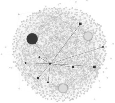
Figure 1: Peer-grading network: Each node is a learner with edges depicting who graded whom. Node size represents the number of graders for that student. The highlighted learner shown above graded five students (circular nodes) and was in turn graded by four students (square nodes).

Initial MOOC-scale peer grading experiments have shown promise. A recent offering of an online Human Computer Interaction (HCI) course demonstrated that on average, student grades in a MOOC exhibit agreement with staff-given grades [12]. Despite their initial successes, there remains much room for improvement. It was estimated that 43% of student submissions in the HCI course were given a grade that fell over 10 percentage points from a corresponding staff grade, with some submissions up to 70pp from staff given grades. Thus a critical challenge lies in how to reliably obtain accurate grades from peers.

In this paper, we present the largest peer grading networks analysed to date with over $63,000$ peer grades. Our central contribution is to use this unprecedented volume of peer assessment data to extend the discourse on how to create an effective grading system. We formulate and evaluate intuitive probabilistic peer grading models for estimating submission grades as well as grader biases and reliabilities, allowing ourselves to compensate for grader idiosyncrasies. Our methods improve upon the accuracy of baseline peer grading systems that simply use the median of peer grades by over $30\%$ in root mean squared error (RMSE).

In addition to achieving more accurate scoring for peer grading, we also show how fair scores (where our system arrives at a similar level of confidence about every student’s grade) can be achieved by maintaining estimates of uncertainty of a submission’s grade.

Finally we demonstrate that grader related quantities in our statistical model such as bias and reliability have much to say about other educationally relevant quantities. Specifically we explore summative influences: what variables correspond with a student being a better grader, and formative results: how peer grading affects future course participation. With the large amount of data available to us, we are able to perform detailed analyses of these relationships that would have been difficult to validate with smaller datasets.

Because peer grading is structurally similar in both MOOCs and traditional brick and mortar classrooms, these results shed light on best practices across both mediums. At the same time, our work helps to describe the unique dynamics of peer assessment in a very new setting — one which may be part of a future with cheaper, more accessible education.

2 Datasets

In this work, we use datasets collected from two consecutive Coursera offerings of Human Computer Interaction (HCI), taught by Stanford professor Scott Klemmer. The HCI courses used a calibrated peer grading system [16] in order to assess weekly student submissions for assignments which covered a number of different creative design tasks for building a web site. Calibration required students to correctly assess a training submission before they were allowed to grade other students’ submissions. On every assignment, each student evaluated five randomly selected submissions (one of which was a “ground truth” submission, discussed below) based on a rubric, and in turn, was evaluated by four classmates. The final score given to a submission was determined as the median of the corresponding peer grades. Peer grading was anonymized so that students could not see who they were evaluating, or who their evaluators were. See Kulkarni et al. [12] for details of the peer grading system.

After the first offering (HCI1), the peer grading system was refined in several ways. Among other things, HCI2 featured a modified rubric that addressed some of the shortcomings of the original peer grading scheme. Additionally, peer graders were divided into language groups (English and Spanish) to address concerns of being graded by a non-native speaker as well as the observed “patriotic grading effect” [12]. Counting just those who submitted at least one assignment in the English offerings of the class, there were 3,607 students from the first offering (HCI 1) and 3,633 students from the second offering (HCI 2). These students came from diverse backgrounds (with a majority of students from outside of the United States). Collectively, these 7,240 students from around the world created 13,972 submissions, receiving 63,199 peer grades in total. See Table 1 for a summary of the dataset. In our work, we used the data from HCI2 as a hold out set. We formulated our models based only on exploratory experiments performed using the HCI1 dataset, testing on the second HCI class only after having finalized our theories about which models were useful.

Table 1: Data Sets

	First HCI	Second HCI
Students	3,607	3,633
Assignments	5	5
Submissions	6,702	7,270
Peer Grades	31,067	32,132

The software for the peer grading framework used by the HCI courses was designed to accommodate experimental validation of peer grading. A small number (3-5) of submissions for each assignment were marked as “ground truth” and were then graded by the course staff. Since there were only a few ground truth submissions and each student graded at least one per week, the ground truth submissions were “super-graded” and had, on average, 160 assessments. Of note, the students were not told that one of the submissions they were assigned to mark belonged to the ground truth set. For example, Figure 1 shows the network of gradee-grader relationships on Assignment 5 of HCI1, where the three super-graded ground truth submissions are clearly visible.

3 Probabilistic models of peer
grading in MOOCs

The ideal peer grading system for a MOOC should satisfy the following desiderata: it should (1) provide highly reliable/accurate assessment, (2) allocate a balanced and limited workload across students and course staff, (3) be scalable to class sizes of tens or hundreds of thousands of students, and (4) apply broadly to a diverse collection of problem settings. In this section we discuss a number of ways to formulate a probabilistic model of peer grading to address these desiderata. The models that we introduce allow for us to algorithmically compensate for factors such as grader biases and reliabilities while maintaining estimates of uncertainty in a principled way.

Through our paper, we will use the following notation. We refer to the collection of all submissions to a homework assignment as $U$, and specific submissions indexed as $u\in U$. We assume in this paper that each student corresponds to a unique homework submission per assignment, and thus refer to students (users) and submissions interchangeably. The collection of all graders is denoted by $G$, and specific graders by $v\in G$. Note that graders are themselves students with submissions. Finally, we use the notation $v\rightarrow u$ to mean that grader $v$ grades submission $u$. For example, the set $\{u\,:\,v\rightarrow u\}$ refers to the collection of submissions graded by a single student $v$.

Our models assume the existence of the following quantities which are either observed or latent (unobserved) variables which we wish to estimate.

• True scores: We assume that every submission $u$ is associated with a true underlying score, denoted $s_{u}$, which is unobserved and to be estimated.

• Grader biases: Every grader $v$ is associated with a bias, $b_{v}\in\mathbb{R}$. These bias variables reflect a grader’s tendency to either inflate or deflate her assessment by a certain number of percentage points.

• Grader reliabilities: We also model grader reliability, $\tau_{v}\in\mathbb{R}^{+}$, reflecting how close on average a grader’s peer assessments tend to land near the corresponding submission’s true score after having corrected for bias. In the models below, $\tau_{v}$ will always refer to the precision, or inverse variance of a normal distribution.

• Observed grades: Finally, $z^{v}_{u}\in\mathbb{R}$ is the observable score given by grader $v$ to submission $u$. The collection of all observed peer grades is denoted as $Z=\{z^{v}_{u}\}$.

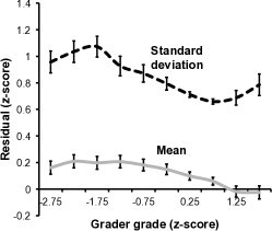
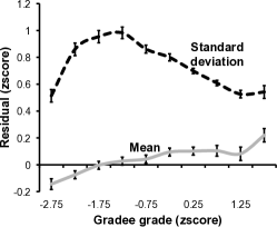
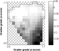
Figure 2: 2 The relationship between a grader’s homework performance (her grade) and statistics (mean/standard deviation) of grading performance (residual from true grade). 2 The relationship between a gradee’s homework performance against statistics of assessments for her submissions. 2 Visualization of all three variables simultaneously, where intensity reflects the mean residual $z$-score. Empty boxes mean that there is not enough data available to compute a reliable estimate.

3.1 Models

Below we present, in order of increasing complexity, three statistical models that we have found to be particularly effective.

Model $\mbox{\bf PG}_{1}$ (Grader bias and reliability)

Our first model, $\mbox{\bf PG}_{1}$ puts prior distributions over the latent variables and assumes for example that while an individual grader’s bias may be nonzero, the average bias of many graders is zero. Specifically,

$$\mbox{(Reliability)}\;\tau_{v} \sim\mathcal{G}(\alpha_{0},\,\beta_{0})\;\mbox{for every grader $v$},$$

$$\mbox{(Bias)}\;b_{v} \sim\mathcal{N}(0,\,1/\eta_{0})\;\mbox{for every grader $v$},$$

$$\mbox{(True score)}\;s_{u} \sim\mathcal{N}(\mu_{0},\,1/\gamma_{0})\;\mbox{for every user $u$, and}$$

$$\mbox{(Observed score)}\;z^{v}_{u} \sim\mathcal{N}(s_{u}+b_{v},\,1/\tau_{v}),$$

for every observed peer grade.

$\mathcal{G}$ refers to a gamma distribution with fixed hyperparameters $\alpha_{0}$, $\beta_{0}$, while $\eta_{0}$, and $\gamma_{0}$ are hyperparameters for the priors over biases and true scores, respectively. In our experiments, we also consider a simplified version of Model $\mbox{\bf PG}_{1}$ in which the reliability of every grader is fixed to be the same value. We refer to this simpler model in which only the grader biases are allowed to vary as $\mbox{\bf PG}_{1}$-bias .

Model $\mbox{\bf PG}_{2}$ (Temporal coherence)

The priors for reliability and bias can play a particularly important role in the above model due to the fact that we typically only have about 4-5 grades to estimate the bias and reliability of each grader. A simple way to obtain more data per grader is to leverage observations made about the grader from previous assignments. To pose a model, we must understand the relationship of a grader’s bias and reliability at homework $T$ to that at homework $T^{\prime}$. Is it the same or does it change over time?

To answer this question, we examine the correlation between the estimated biases from Model $\mbox{\bf PG}_{1}$ using the HCI1 dataset (see Section 2). Between consecutive assignments, a grader’s biases have a Pearson correlation of 0.33 which represents a utilizable consistency. Grader reliability, on the other hand, has a low correlation. We therefore posit Model $\mbox{\bf PG}_{2}$ which allows for grader biases at homework $T$ to depend on those at homework $T-1$ (and implicitly, on all prior homeworks). Specifically, Model $\mbox{\bf PG}_{2}$ assumes:

$$\tau_{v}^{(T)} \sim\mathcal{G}(\alpha_{0},\beta_{0})\;\mbox{for every grader $v$},$$

$$b_{v}^{(T)} \sim\mathcal{N}(b_{v}^{(T-1)},1/\omega_{0})\;\mbox{for every grader $v$},$$

$$s_{u}^{(T)} \sim\mathcal{N}(\mu_{0},1/\gamma_{0})\;\mbox{for every user $u$, and}$$

$$z^{v,(T)}_{u} \sim\mathcal{N}(s_{u}^{(T)}+b_{v}^{(T)},1/\tau_{v}^{(T)}),$$

for every observed peer grade.

Model $\mbox{\bf PG}_{2}$ requires that we normalize grades across different homework assignments to a consistent scale. In our experiments, for example, we have noticed that the set of grader biases had different variances on different homework assignments. Using a normalized score ($z$-score), however, allows us to propagate a student’s underlying bias while remaining robust to assignment artifacts.

Note that while a model which captures the dynamics of true scores and reliabilities across assignments can be similarly imagined, we have focused only on the dynamics of bias for this work (which contributes the most towards improved accuracy while still being equitable).

Model $\mbox{\bf PG}_{3}$ (Coupled grader score and reliability)

A unique aspect of peer grading is that graders are themselves students with submissions being graded. Consequently, it is of interest to understand and model the relationship between one’s grade and one’s grading ability — for example, knowing that a student scored well on his assignment may be cause for placing more trust in that student as a grader, and vice versa.

In Figure 2, we show experiments exploring the relationships between the grader specific latent variables. In particular, we observe that high scoring students tend to be somewhat more reliable as graders (see details of the experiment in Section 4). Model $\mbox{\bf PG}_{3}$ formalizes this intuition by allowing the reliability of a grader to depend on her own grade, and assumes the following:

$$b_{v} \sim\mathcal{N}(0,\,1/\eta_{0})\;\mbox{for every grader $v$},$$

$$s_{u} \sim\mathcal{N}(\mu_{0},\,1/\gamma_{0})\;\mbox{for every user $u$, and}$$

$$z^{v}_{u} \sim\mathcal{N}\left(s_{u}+b_{v},\,\frac{1}{\theta_{1}s_{v}+\theta_{0}}\right),$$

for every observed peer grade.

Note that Model $\mbox{\bf PG}_{3}$ extends $\mbox{\bf PG}_{1}$ by introducing new dependencies, allowing us to use a student’s submission score to estimate her grading ability. At the same time Model $\mbox{\bf PG}_{3}$ is more constrained, forcing grader reliability to depend on a single parameter instead of being allowed to vary arbitrarily, and thus prevents our model from overfitting.

Ethics and Incentives

If we are to use probabilistic inference to score students in a MOOC, the end goal could not simply be to optimize for accuracy. We must also consider fairness when it comes to deciding what variables to include in the model. It might be tempting, for example, to include variables such as race, ethnicity and gender into a model for better accuracy, but almost everyone would agree that these factors could not be fairly used within a scoring mechanism even if they improved prediction accuracy. Another example might be to model the temporal coherence of student grades (we observe a particularly strong temporal correlation between students’ grades — with 0.46 Pearson coefficient — of consecutive homework assignments). But incorporating this temporal coherence for students scores into a scoring mechanism would not allow for students to be given a “clean slate” on each homework.

Model $\mbox{\bf PG}_{3}$ allows for the inferred true score of a submission to depend on graders’ scores, which may seem contentious, but the dependence is weak, only affecting the influence by a particular grader on the final prediction, which is desirable. Interestingly, using the more complex scoring mechanism from Model $\mbox{\bf PG}_{3}$ may in fact incentivize for good grading. In particular, a student’s grade is influenced by how closely her assessments as a grader match those of other graders who graded the same assignments. Consequently, by allowing for student grades to depend on their performance as graders, Model $\mbox{\bf PG}_{3}$ used as a scoring mechanism may incentive students to put more effort into grading.

3.2 Inference and evaluation.

Given a probabilistic model of peer grading such as those discussed above, we would like to infer the values of the unobserved variables such as the true score of every submission, or the bias and reliability of each student as a grader. Inference can be framed as the problem of computing the posterior distribution over the latent variables conditioned on all observed peer grades (e.g., $P(\{s_{u}\}_{u\in U},\{b_{v}\}_{v\in G},\{\tau_{v}\}_{v\in G}\;|\;Z)$).

Computing this posterior is nontrivial, since all of the variables are correlated with each other. For example, having good estimates of the biases of all of the graders to submission $u$ ($\{b_{v}:v\rightarrow u\}$) would allow us to better estimate $u$’s true score, $s_{u}$. However to estimate each bias $b_{v}$, we would have to have good estimates of the true scores of all of the submissions graded by $v$ ($\{s_{u}:v\rightarrow u\}$). We must therefore reason circularly, in that — if we knew every submission’s true scores, we would be able to easily compute posterior distributions over grader biases (and reliabilities), but in order to estimate these biases, we must know the true score of each submission.

To address this apparent chicken and egg problem, we turn to simple approximate inference methods. In the experiments reported in Section 4, we use Gibbs sampling [6], which produces a collection of samples from the (approximate) desired posterior distribution. These samples can then be used to estimate various quantities of interest. For example, given samples $s^{1}_{u},s^{2}_{u},\dots,s^{T}_{u}$ from the posterior distribution over the true score of submission $u$, we estimate the true score as: $\hat{s}_{u}\equiv\frac{1}{T}\sum_{t=1}^{T}s^{t}_{u}$. We can also use the samples to quantify the uncertainty of our prediction by estimating the variance of the samples from the posterior, which we use in Section 4 when we examine peer grading efficiency. Note that while the ordinary Gibbs sampling algorithm can be performed in “closed form” for Models $\mbox{\bf PG}_{1}$-bias , $\mbox{\bf PG}_{1}$ and $\mbox{\bf PG}_{2}$ , Model $\mbox{\bf PG}_{3}$ requires numerical approximation due to the coupling of a submission’s true score $s_{u}$ with that of its grader, $s_{v}$. We discuss details in the Appendix. Visually we observe rapid mixing for our Gibbs chains, and in the experiments shown in Section 4, we use 800 iterations of Gibbs sampling, discarding the initial 80 burn-in samples.

Expectation-maximization (EM) is alternative approximate inference approach, where we treat the true scores and grader biases as parameters and then use an iterative coordinate descent based algorithm to obtain point estimates of parameters. In practice, we find that both the Gibbs and EM approaches behave similarly. In general EM has the advantage of being significantly faster while obtaining posterior credible intervals is more natural using Gibbs. On the peer grading dataset the two methods produce analogous results. For example, $\mbox{\bf PG}_{1}$ with Gibbs and EM have RMSE scores of 5.42 and 5.43 on the first dataset respectively and with Gibbs running in roughly 5 minutes and EM running in 7 seconds. We refer the reader to the appendix for the full algorithmic details of Gibbs as well as EM.

Table 2: Comparison of models on the two HCI courses

	HCI 1						HCI 2
	Baseline	$\mbox{\bf PG}_{1}$-bias	$\mbox{\bf PG}_{1}$	$\mbox{\bf PG}_{2}$	$\mbox{\bf PG}_{3}$		Baseline	$\mbox{\bf PG}_{1}$-bias	$\mbox{\bf PG}_{1}$	$\mbox{\bf PG}_{2}$	$\mbox{\bf PG}_{3}$
RMSE	7.95	5.42	5.40	5.40	5.30		6.43	4.84	4.81	4.75	4.73
% Within 5pp	51	69	69	71	70		59	72	73	73	74
% Within 10pp	81	92	94	94	95		88	96	96	97	97
Mean Std	7.23	5.00	4.96	4.92	4.77		6.19	4.57	4.52	4.53	4.52
Worst Grade	-43	-34	-30	-32	-30		-36	-26	-26	-25	-26

Evaluation

To measure peer grading accuracy, we repeatedly simulate what score would have been assigned to each ground truth submission had it been peer graded. Our evaluation of how well we would have graded a single ground truth submission uses a two step methodology (based on the evaluation method of [12]): (1) We run inference using all of our data, except the peer grades of the ground truth submission being evaluated. This gives us an estimate of each grader’s biases and reliabilities as well as model priors that were independent of the submission being evaluated. (2) We run simulations where we sampled four student assessments randomly from the pool of peer grades for the ground truth submission, estimate the submission’s grade using the sample of assessments and recorde the residual between our estimated grade and the “true” grade. For each ground truth submission we run 3000 such simulations, from which we report the RMSE, the number of simulations which fell within five, and ten percentage points of the true score, the average standard deviation of the errors over each ground truth and the worst misgrade that the simulations produced.

An interesting issue is whether one should consider the “true” grade of a ground truth submission to be the score given by the staff, or the consensus from the hundreds of students that assessed the submission. For our datasets, we believe that the discrepancy between staff grade and student consensus typically results from ambiguities in the rubric and elect to use the mean of the student consensus on a ground truth submission as the true grade. One interesting observation that came from our exploration: peer graders in our datasets have a tendency to grade towards the mean, inflating grades for low-scoring submissions and deflating grades for high-scoring submissions. We remark that while our experiments were run in an “unsupervised” fashion, it would be reasonable to use staff grades in the training process in order to encourage the model to place more trust in students who consistently grade like the instructors.

We compare each of our probabilistic models to the grade estimation algorithm used on Coursera’s platform. In the baseline model, the score given to students is the median of the four peer grades they received. Specifically, the baseline estimation does not take into account individual grader’s biases and reliabilities. Nor does it incorporate prior knowledge about the distribution of true grades.

4 Experimental results

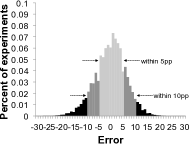
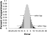
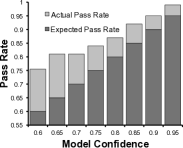
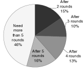
Figure 3: 3 Histogram of errors made using the baseline (median) scoring mechanism. 3 Histogram of errors using $\mbox{\bf PG}_{3}$ . 3 A comparison of model confidence ($x$-axis) and actual success rate of predictions ($y$-axis), where being above the diagonal (dark bars) is better. 3 Number of submissions for which our model can declare “confidence” after $K$ rounds of grading.

4.1 Accuracy of reweighted peer grading

Using probabilistic models leads to substantially higher grading accuracy. In our experiments we are able to reduce the RMS error on our prediction of the ground truth grade by 33% from 7.95 to 5.30. Similarly, on the second offering of the course we were able to reduce error by 31% from 6.43 to 4.73. For the second offering, this means that the number of students who received grades within 10 percentage points (pp) of their grade increased from 88% to 97%. Figures 3, 3 show the effect of using Model  $\mbox{\bf PG}_{3}$ as a scoring mechanism on the histogram of grading errors and Table 2 shows the complete results for each model. Due to course improvements, we observe that students in HCI2 were significantly more consistent as graders compared to students in HCI1. However, we remark that every one of our models run on HCI1 outperforms the baseline grading system run on HCI2 with respect to every metric, indicating that the best gains in peer grading are likely to come from both an improved class design as well as statistical modeling.

Our results show that Models $\mbox{\bf PG}_{3}$ (with coupled grader score and reliability) and $\mbox{\bf PG}_{2}$ (with temporal coherence) yield the best results, with Model $\mbox{\bf PG}_{3}$ outperforming the other models with respect to most metrics. But the single change that provides the most significant gains in accuracy is obtained by estimating each grader’s bias (Model $\mbox{\bf PG}_{1}$-bias ). This simple model is responsible for 95% of our reduction in RMSE. The other changes all contribute comparatively smaller improvements to a more accurate model.

Our evaluation setup also allows us to test how accurate we would have been, had we had more than four grades per student. If the class had increased the number of grades that each student received to five (instead of four), our model could reduce RMSE error on the first and second offering of HCI to 4.19 and 4.36 respectively.

Surprisingly while modeling grader bias is particularly effective, modeling grader precision does little to improve our performance. To dig deeper into this result we test our model on a synthetic dataset — one generated exactly from Model $\mbox{\bf PG}_{1}$ . When using this synthetic data with only four grades per student it is difficult for the model to correctly estimate grader reliability. Modeling variance for each grader only seems to have a notable impact when students grade many assignments (more than 10). This experiment also suggests why $\mbox{\bf PG}_{3}$ is more useful than $\mbox{\bf PG}_{1}$ . Though $\mbox{\bf PG}_{1}$ contains more expressive power than $\mbox{\bf PG}_{3}$ , estimating only two parameters for grader reliability ($\theta_{0}$ and $\theta_{1}$) is more statistically tractable with only four grades per student than estimating a reliability, $\tau_{v}$, for each grader.

4.2 Fairness and efficiency in peer grading

One of the advantages of using a probabilistic model for peer grading is that we can obtain a belief distribution over grades (as opposed to a single score) for each student. These distributions give us a natural way of calculating how confident the model is when it predicts a grade for a student. The fact that the confidence results can be trusted open up the possibility of a more equitable allocation of graders. For example, at a given point midway through the peer grading process, our model may be highly confident in its prediction for a given student’s score, but very unsure in its prediction for another student. In this situation, to ensure that each student gets fair access to quality feedback, we could reassign graders to gradees such that submissions which have low-confidence scores are given to more and/or better graders.

The first step towards more fair allocation of grades is to ask ourselves: how accurate are our estimates of confidence? For example, we would like to know how to interpret what it means in practice when our Bayesian model is 90% confident that its prediction of a learner’s true score is within 10pp of the actual true score.

To better understand our confidence estimates, we run the following experiment: We first performed a large number of peer grading simulations on ground truth. From each simulation we calculate how confident our model is that the grade it predict for the ground truth submission is within 5%, 7%, and 10%, of the true score, respectively. We then bin the estimated confidences into ranges 0-5%, 5-10%, etc. After collecting over 5000 predictions per range, we test the pass rate of each range. For example, suppose we select four assessments of the same ground truth submission in a simulation. If our model reports a 72% confidence — based on those four assessments — that our predicted grade is within 5pp of the true score, we add that estimate to the set of predictions in the 70% to 75% confidence range. When we test this confidence range the example prediction “passes” if its estimate is in fact within 5pp of the ground truth score.

One worry is that our model might be overconfident about its predictions even when wrong. However the results, shown in Figure 3, demonstrate that our confidence estimates are on the conservative side — for example over 95% of the time that our model claims it is between 90 and 95% confident of a prediction, the model’s estimate is correct.

Since we have reason to believe that our confidence values are accurate, we can employ our posterior belief distributions to better allocate grades. To understand how much benefit we could get out of improved grade allocation, we estimate at what point in the grading process we were confident about each submission’s score. For each homework assignment, we simulate grading taking place in rounds. In the first round, we only include the first grade submitted by each grader (which may have been a ground truth grade). In the second round, we included the first two, etc. For each round we run our model using the corresponding subset of grades and count the number of submissions for which we are over 90% confident that our predicted grades were within 10pp of the student’s true grade.

After only two rounds of grading we are highly confident in our estimated grade for 15% of submissions (this generally means that the submission has a grade close to the assignment mean, and has two similar grades from graders). Figure 3 shows how the set of confident submissions grows over the grading rounds. Our experiment demonstrates a clear opportunity for grades to be reallocated as well as a pressing need for some submissions to get more grades. For 54% of students, after all rounds, we are still unsure of their submission’s true score.

4.3 Graders in the context of the MOOC

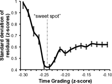
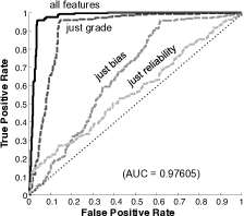
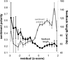
Figure 4: 4 Grader consistency (measured using standard deviation of grading residual) as a function of time spent grading. 4 ROC curve comparing performance (with linear SVM) at predicting future class participation given a student’s grade, bias, reliability or all three. 4 Commenting style (length of comment and sentiment polarity) as a function of grading residual.

Applying probabilistic models to peer grading networks allows us to increase our grade accuracy and better allocate what submissions students should grade. Another product of our work is an assignment — with a belief distribution — for a true score, grader bias and grader reliability for each student. We can use this large dataset to derive new understanding about peer grading as both a formative and summative assessment. We focus our investigation on two questions, (1) what factors influence how well a student grades? and (2) how does grading ability affect future class performance in a MOOC?

Influential factors for grader ability

To explore what factors influence how well a student grades we compare grading residual (how far off a grader’s score is from our model estimated true score) to: time spent grading, grader grade, and gradee grade.

Time spent grading shows a particularly interesting trend (Figure 4). As hypothesized, students that “snap grade” their peers’ work (the students whose time spent grading has a $z$-score of less than -0.30), are both unreliable (the variance of their residuals is over 1 standard deviation away from the gradee’s true score) and tend to slightly inflate grades. More surprising is that over the tens of thousands of grades, there is a “sweet spot” of time spent grading. Students who grade assessments with a time that has a $z$-score of around -0.25 have significantly lower residual standard deviations (with $p$-value < 0.001, diff = 0.3 standard deviations) than students who take a long time to grade (i.e., time spent grading has a $z$-score > -0.20). This sweet spot is only visible when we look at normalized grading times. For most assignments in the HCI class, the sweet spot corresponds to around 20 minutes grading. This may reflect both that with any less time a grader does not have enough of a chance to fully examine her gradee’s work, and that a long grading session may mean that the grader had trouble understanding some facet of the submission.

Examining the relationship between grader grade, gradee grade and how they affect the residual also shows a set of notable trends. Graders that score higher on assignments have close to monotonically decreasing biases (Figure 2). Getting a better grade on the homework in general makes students more reliable graders; with the notable exception that the students that get the best grades (+1.75 $z$-score) are not as accurate as the students who do very well (+.75 $z$-score, $p$ = 0.04). The superlative submissions — both the best and the worst — are the easiest to grade, and the submissions which are one standard deviation below the mean are the hardest (Figure 2). Finally, our results show that students are least biased when grading peers with similar score (Figure 2). The best students significantly downgrade the worst submissions and the worst students notably inflate the best submissions.

In addition to numerical scores, graders were asked to provide feedback in the form of free form text comments to their gradees. In order to understand the relationship between grading performance and commenting style, we compare grading residual against the comment length as well as sentiment polarity of the comment (Figure 4). To measure the polarity of a comment, we use the sentiment analysis word list from [14] and implement a simple sentiment analyzer that returns a (normalized) polarity score (positive or negative) proportional to the sum of word valences over the comment. For both comment length and polarity, we filter out all non-English words. We observe that comments that correspond to larger negative residuals are typically significantly longer, suggesting perhaps that students write more about the weaknesses of a submission than strong points. That being said, we observe that overall, the comments mostly range in polarity from neutral to quite positive, suggesting that rather than being highly negative to some submissions, many students make an effort to be balanced in their comments to peers.

Grader ability and future performance

We also tested what signal grading ability has with predicting future participation. Based on the theory that the best graders are intrinsically motivated, we hypothesized that being a reliable grader would add a different dimension of information to a student’s engagement which we should be able to use to better predict future engagement. We tested this hypothesis by constructing a classification task in which we predict whether a student would participate in the next assignment (or conversely which students would “drop out”). In addition to the student’s grade, we experimented with including grader bias and reliability as features in a linear classifier. Our results (Figure 4) show that including grader bias and reliability improved our predictive ability by 5pp from an area under the curve (AUC) score of 0.93 to an AUC of 0.98. Properties about how a student grades, captures a dimension of their engagement which is missed by their assignment grade.

5 Related work

The statistical models we present in this paper can be seen as part of a long tradition of models which have been proposed for the purposes of aggregating information from noisy human labelers or workers. Many of these works adapt classical item-response theory (IRT) models [3] to the problem of “grading without an answer key” and appear in the literature from educational aptitude testing [9, 15, 13], to cultural anthropology [4, 11], and more recently to HCI in the context of human computation and crowdsourcing [18]. In educational testing, for example, Johnson [9] and Rogers et al. [15] propose models for combining human judgements of essays. These papers analyze dedicated human graders who each evaluated hundreds of essays, allowing for a rich model to be fitted on a per-grader basis. In contrast, with peer grading in MOOCs, each student only assesses a handful of assignments, necessitating more constrained models.

In a recent paper, and in a setting perhaps most similar to our own, Goldin et al. [8, 1, 7] use Bayesian models for peer grading in a smaller scale classroom setting. As in our own work, [7] posits a grader bias, and in fact incorporates rubric-specific biases, but does not consider many of the issues raised here such as grading task reallocation or the relationship between grader bias and student engagement, for example.

One of the central themes of the crowdsourcing literature, that of balancing label accuracy against labor cost, is one which MOOC peer grading systems must contend with as well. In such problems, one typically receives a number of noisy labels (for example in an image tagging task) and the challenge lies in (1) resolving the “correct” label (often discrete, but sometimes continuous) and (2) deciding whether to hire more labelers for a given task. Explosion of interest in recent years has led to widespread applications of crowdsourcing [2, 10]. For example in image annotation, Whitehill et al. [18] present a method similar to our own in which they model discrete “true image labels” as well as labeler accuracy. While our work draws from the crowdsourcing literature, the problem of peer grading is unique in several ways. For example, the fact that the graders are also gradees in peer grading is quite different from typical crowdsourcing settings in which there is a dichotomy between the labelers and the items being labeled, and motivates different models (such as Model $\mbox{\bf PG}_{3}$ ). In crowdsourcing applications, the end goal often lies in determining the true labels rather than to understand anything about the labelers themselves, whereas in peer grading, as we have shown, the insights that we can glean about the graders have educational value.

A similar problem to peer-grading is the paper assignment problem for the peer review process in academic conferences. While related in that the central challenge of both problems involves fusing disparate human opinions about open-ended creative work, many of the specific challenges are distinct. For one, side information plays a much larger role in peer review, where conference chairs typically rely heavily on personal or elicited knowledge of reviewer expertise or citation link structure to assign reviewer roles [5]. Peer grading on the other hand seems less sensitive to personal preferences, where a single submission should be equally well graded by a large fraction of students in the course.

6 Discussion and Future work

Our paper presents methods for making large scale peer grading systems more dependable, accurate, and efficient. In particular, we show that there is much to be gained by maintaining estimates of grader specific quantities such as bias and reliability. In addition to improving peer grading accuracy by up to 30%, these quantities give a unique insight into peer grading as a formative and summative assessment.

There remain a number of issues to be addressed in future work. We have considered the problem of determining which submissions need to be allocated additional graders. However, deciding which grader is best for evaluating a particular submission is an open problem whose solution could depend on a number of variables, from the writing styles of the grader and gradee to their respective cultural or linguistic backgrounds, a particularly important issue for the global scale course rosters that arise in MOOCS.

Another issue arises from our study of the biases from graders who do not spend adequate time on grading. Incentivizing these students to provide careful and high quality feedback to their peers is a question of paramount importance for open-access courses. Using model $\mbox{\bf PG}_{3}$ for scoring, as we discussed, makes a student’s score dependent on grading performance, and may be one way to build a justified, incentive directly into the scoring mechanism. Understanding this and other scoring rules from a game theoretical perspective remains for future work.

Finally, it is not clear how to present scores which are calculated by a complicated peer grading model to a students. While this communication might be easy when a student’s final grade is simply set to be the mean or median of peer grades, does each student need to know the inner workings of a more sophisticated statistical backend? Students may be unhappy with the lack of transparency in grading mechanisms, or on the other hand might feel more satisfied with their overall grade.

As MOOCs become more widespread, the need for reliable grading and feedback for open ended assignments becomes ever more critical. The most scalable solution that has been shown to be effective is peer grading. By addressing the shortcomings of current peer grading systems, we hope that students everywhere can get more from peer grading and consequently, more from their free online, open access educational experience.

References

- [1] K. Ashley and I. Goldin. Toward ai-enhanced computer-supported peer review in legal education. In 24th International Conference on Legal Knowledge and Information Systems (JURIX), volume 235, 2011.
- [2] Y. Bachrach, T. Minka, J. Guiver, and T. Graepel. How To Grade a Test Without Knowing the Answers - A Bayesian Graphical Model for Adaptive Crowdsourcing and Aptitude Testing. In The 29th Annual International Conference on Machine Learning, ICML ’12, 2012.
- [3] F. Baker. The basics of item response theory. ERIC Clearinghouse on Assessment and Evaluation, University of Maryland, College Park, 2001.
- [4] W. H. Batchelder and A. K. Romney. Test theory without an answer key. Psychometrika, 53:71–92, 1988.
- [5] L. Charlin, R. Zemel, and C. Boutilier. A framework for optimizing paper matching. In Proceedings of Uncertainty in Artificial Intelligence (UAI’11), 2011.
- [6] S. Geman and D. Geman. Stochastic relaxation, gibbs distributions, and the bayesian restoration of images. IEEE PAMI, (6):721–741, 1984.
- [7] I. Goldin. Accounting for peer reviewer bias with bayesian models. In Proceedings of the Workshop on Intelligent Support for Learning Groups at the 11th International Conference on Intelligent Tutoring Systems, 2012.
- [8] I. M. Goldin and K. D. Ashley. Peering inside peer review with bayesian models. In Proceedings of the 15th international conference on Artificial intelligence in education, AIED’11, pages 90–97, Berlin, Heidelberg, 2011. Springer-Verlag.
- [9] V. E. Johnson. On bayesian analysis of multi-rater ordinal data: An application to automated essay grading. Journal of the American Statistical Association, 91:42–51, 1996.
- [10] E. Kamar, S. Hacker, and E. Horvitz. Combining human and machine intelligence in large-scale crowdsourcing. In In AAMAS, 2012.
- [11] G. Karabatsos and W. Batchelder. Markov chain estimation for test theory without an answer key. Psychometrika, 68(3):373–389, 2003.
- [12] C. Kulkarni, K. Pang-Wei, H. Le, D. Chia, K. Papadopoulos, D. Koller, and S. R. Klemmer. Scaling self and peer assessment to the global design classroom. In Proceedings of CHI’13 (to appear), 2013.
- [13] R. J. Mislevy, R. G. Almond, D. Yan, and L. S. Steinberg. Bayes nets in educational assessment: Where the numbers come from. In Proceedings of the fifteenth conference on uncertainty in artificial intelligence, pages 437–446. Morgan Kaufmann Publishers Inc., 1999.
- [14] F. Å. Nielsen. A new anew: Evaluation of a word list for sentiment analysis in microblogs. arXiv preprint arXiv:1103.2903, 2011.
- [15] S. Rogers, M. Girolami, and T. Polajnar. Semi-parametric analysis of multi-rater data. Statistics and Computing, 20(3):317–334, July 2010.
- [16] A. A. Russell. Calibrated peer review - a writing and critical-thinking instructional tool. Teaching Tips: Innovations in Undergraduate Science Instruction, page 54, 2004.
- [17] P. M. Sadler and E. Good. The impact of self-and peer-grading on student learning. Educational assessment, 11(1):1–31, 2006.
- [18] J. Whitehill, P. Ruvolo, T. fan Wu, J. Bergsma, and J. Movellan. Whose vote should count more: Optimal integration of labels from labelers of unknown expertise. In Advances in Neural Information Processing Systems 22, pages 2035–2043. MIT Press, 2009.