Abstract

We are concerned with the complexity reduction of a stochastic system of differential equations governing the dynamics of a neuronal circuit describing a decision-making task. This reduction is based on the slow-fast behavior of the problem and holds on the whole phase space and not only locally around the spontaneous state. Macroscopic quantities, such as performance and reaction times, computed applying this reduction are in agreement with previous works in which the complexity reduction is locally performed at the spontaneous point by means of a Taylor expansion.

Author Summary

In recent years, the neuronal mechanisms governing binary decision-making have largely been studied. In a wide range of experiments, the behavioral response can be described by means of stochastic systems. In particular, we are interested in the qualitative analysis of the performance and reaction times corresponding to a decision-making problem. In order to perform the link between neuronal circuits and stochastic systems, we consider here a mean-field reduction consisting of two interacting rate models. This system of equations can be associated with a partial differential equation governing the probability distribution of the activities of the different neuronal populations. However, the nonlinear nature of the original equations hinders analytical progress in the partial differential framework and reduces its study to numerical investigations having very large computational times. We propose here a complexity reduction of the stochastic system, based on its slow-fast characteristic, allowing us to define a solution on the whole biological domain, rather than just on a neighborhood of the spontaneous state, as it is usually done. Moreover, close to the bifurcation point, the qualitative behavior of the performance and reaction times is the same as the one observed in previous works.

Introduction

Goal-oriented behavior involves the constant making of decisions between alternative choices. Hence, a sorrow understanding of the mechanisms underlying decision-making is fundamental in behavioral neurosciences. During the last years tremendous advances in neurophysiological and theoretical neurosciences have started to reveal the neural mechanisms underlying decision-making. Most of these studies are focused on binary decision-making. In binary decision tasks, the subject is asked to make a choice between two alternatives according to an experimentally defined criterion based on sensory input information. The difficulty of the making of the decision can be manipulated by the level of uncertainty in the discrimination of the sensory input information which can be influenced by regulating the signal to noise ratio. For the same pattern of stimulation the decision of the subject from trial-to-trial is stochastic but such that its trial-to-trial average is determined by the input.

In a wide range of such decision-making experiments, the behavioral response, i.e. performance and reaction times, can be properly described by a simple stochastic diffusion model [1]. In the diffusion model evidences about one or the other choice is accumulated continuously over time until a decision boundary is reached. Hence, it is plausible to think that the underlying neuronal system perform decision-making by accumulation of evidences. Indeed, recent electrophysiological recordings from awake behaving monkeys performing decision-making have shown that trial-averaged spiking activity of some neurons shows a gradual, nearly linear increase shortly after stimulus onset until just before the response is made [2, 3, 4, 5, 6]. Let us consider for example the so-called random-dot task. The random-dot task is a two-choice visual decision-making task. In this task, the subject is confronted with a visual stimulus consisting of a field of randomly moving dots. On any one trial, a fixed fraction of the dots, determined by the experimentalist, moves coherently in one of two directions. The subject must discriminate in which direction the majority of dots are moving. Electrophysiological recordings from awake behaving monkeys performing this task have shown that trial-averaged spiking activity of neurons in the lateral intraparietal cortex (LIP) reflects the accumulation of information mentioned above [4, 5, 6]. In fact, LIP cells receive excitatory drive from direction-selective cells of extrastriate visual area MT. The difference in the firing rates of MT cells with opposing preferred directions is a likely measure of the available visual evidence for the direction of coherent motion of the moving dot stimulus, further indicating that the LIP area is involved in this decision-making task.

A computational model of the cortical circuit putatively underlying LIP cell activity has been proposed and studied numerically [7, 8, 9]. This model was able to explain qualitatively the experimentally observed trial-averaged spiking activity. The model consists of two populations of spiking neurons, within which interactions are mediated by excitatory synapses and between which interactions occur principally through an intermediary population of inhibitory interneurons. Sensory input may bias the competition in favor of one of the populations, potentially resulting in a gradually developing decision in which neurons in the chosen population exhibit increased activity while activity in the other population is inhibited. When the activity of one of the two populations exceeds a pre-defined threshold then a behavioral response is generated. There are two possible mechanisms by which the decision can be made which correspond to two different dynamical working points. In one mechanism, the appearance of the stimulus destabilizes the so-called spontaneous state, in which all neurons show low activity. In the other mechanism, even after stimulus presentation, the network can still sustain low activity, but random fluctuations eventually drive the collective activity of the network to an activated state, in which a fraction of the neurons fires at a high rate. Let us remark that the behavioral performance of the model (i.e. the fraction of trials in which the ’correct’ direction is chosen) and corresponding reaction time to make a decision match well the behavioral data from both monkeys and humans performing the moving-dot task [10]. Therefore, we conjecture, that it may be possible to establish a direct link between the neuronal and behavioral correlates of decision-making. Here, we aim to establish this link between the underlying physiology and the observed behavioral response in decision-making tasks by performing a 1D reduction of the dynamics of the neuronal circuit in such a way that we derive from the underlying detailed neuronal dynamics a valid ”nonlinear” diffusion model.

In order to perform the explicit link between a neuronal circuit processing decision-making and a diffusion model able to describe the behavioral level, we consider a reduced model of the competitive cortical circuit solving the decision-making problem. In particular, we consider a mean-field reduction consisting of two competing rate models. This system of Langevin equations can be associated with a Fokker-Planck equation for the probability distribution of the activities of the different neuronal populations. The nonlinear nature of the original equations, however, hinders analytical progress in the Fokker-Planck framework. For this reason, the main analysis of such noise driven probabilistic decision-making systems remains based on numerical investigations, which are time consuming because of the need for sufficiently many trials to generate statistically meaningful data.

One dimensional Fokker-Planck effective reductions near bifurcation points were obtained by Roxin and Ledberg [10]. They propose to locally approximate the evolution on the slow manifold at the bifurcation point by Taylor expanding the nonlinearities with respect to the slow variable based on the different time scales. In this way, they obtained an effective potential of degree 4 for the one dimensional Fokker-Planck dynamics on the slow manifold. We propose to build on this strategy by not performing any Taylor expansion and rather approximate the slow manifold in terms of the nonlinearities defining the evolution using the slow-fast character of the dynamical system, see [11]. Once, the slow manifold is approximated then we project the Fokker-Planck dynamics on it to obtain a one dimensional Fokker-Planck reduction possibly valid beyond the local character of the expansion in [10]. More importantly, we recover an approximated full reduced potential and an explicit formula for the stationary state distribution on the slow manifold. This effective reduced potential covers the other two stable equilibrium points, and not only the central equilibrium point changing its stability character as in [10]. For instance, in the case of the subcritical Hopf bifurcation in Figure 1, we get an approximated potential as in Figure 5 while the approach in [10] leads to a potential of degree 4 approximating an interval around the central equilibrium point, see [10, Figure 2]. Our strategy is valid as long as the approximated slow manifold lies fully in the relevant biological range of positive rates, this is the reason we restrict the range of the bifurcation parameter $w_{+}$ as explained in Figure 3.

Results

We showcase our strategy in a particular example of a neuronal population model with two pools with self-excitation and cross-inhibition as in [12]. The firing rates $\nu_{1}$ and $\nu_{2}$ of the neuronal networks are determined by the stochastic dynamical system:

$$\begin{cases}{d\nu_{1}}=\left[-\nu_{1}+\phi(\lambda_{1}+w_{+}\nu_{1}+w_{I}\nu_{2})\right]{dt}+\beta\,dW_{t}^{1}\\[8.53581pt] {d\nu_{2}}=\left[-\nu_{2}+\phi(\lambda_{2}+w_{I}\nu_{1}+w_{+}\nu_{2})\right]{dt}+\beta\,dW_{t}^{2}\end{cases},$$ (1)

with $\nu_{1},\nu_{2}\geq 0$. Here the applied stimuli are, $\lambda_{1}=33$, $\lambda_{2}=\lambda_{1}-\Delta\lambda$, with the bias $\Delta\lambda\in[0,10^{-3}]$, the inhibitory connectivity coefficient is $w_{I}=1.9$, the standard deviation is $\beta=3\cdot 10^{-3}$, and the excitatory connectivity coefficient $w_{+}$ is the bifurcation parameter, its range of values will be discussed later on. Moreover, the sigmoid (response) function $\phi(z)$ is given by:

$$\phi(z)=\frac{\nu_{c}}{1+\exp(-bz+\alpha)}\,,$$

with $\nu_{c}=15$, $b=0.25$, and $\alpha=11.1$.

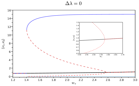
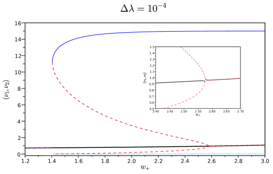
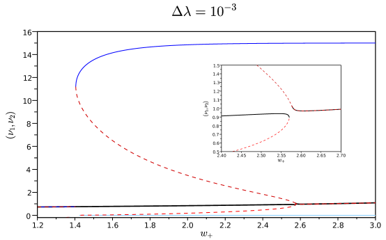
In terms of $w_{+}$ the underlying dynamical system without noise presents a subcritical Hopf bifurcation whose bifurcation diagram is shown in Figure 1. For values of the excitatory coefficient around $w_{+}=1.4$ the system pass from a single asymptotically stable equilibria to a situation in which there are three stable (continuous lines) and two unstable equilibria (hashed lines). The second local bifurcation, where the central asymptotic equilibria disappears, happens at around $w_{+}=2.5695$ for $\Delta\lambda=10^{-3}$.

Figure 1: Bifurcation diagrams with respect to $w_{+}$. From top to bottom the bias $\Delta\lambda$ takes the following values $0,10^{-4}$ and $10^{-3}$. The components of the spontaneous state are traced by the black line. There are other two stable equilibria points which coordinates are represented by the blue and light-blue lines. The red continuous and dashed lines correspond to the unstable equilibrium points. The small picture is a zoom on the bifurcation point.

We next need to find an approximation of the slow manifold joining the spontaneous $S_{0}$ and the decision states $S_{1}$ and $S_{2}$, as sketched in Figure 2. This curve is found by introducing the linearization of the dynamical system around the spontaneous equilibria $S_{0}$ as a new set of variables defined by $X=P^{-1}(\nu-S_{0})$, with $X=(x,y)^{T}$, or equivalently $\nu=S_{0}+PX$ with $\nu=(\nu_{1},\nu_{2})^{T}$. Here, $P$ is the matrix diagonalizing the jacobian of the dynamical system (1) at the spontaneous state $S_{0}$, see (2) in the Materials and Methods section for more details, or [13].

This change of variables, sketched in Figure 2, is a natural way to introduce slow $y$ and fast $x$ variables in the system determined by the eigenvalues of the linearization at the spontaneous state $S_{0}$. By rewriting the dynamical system above (1) in these new variables together with the new time variable $\tau=\varepsilon t$, we have an evolution governed by

$$\begin{cases}\varepsilon\displaystyle\frac{dx}{d\tau}=f(x,y)\\[11.38109pt] \displaystyle\frac{dy}{dt}=g(x,y)\end{cases}\,,$$

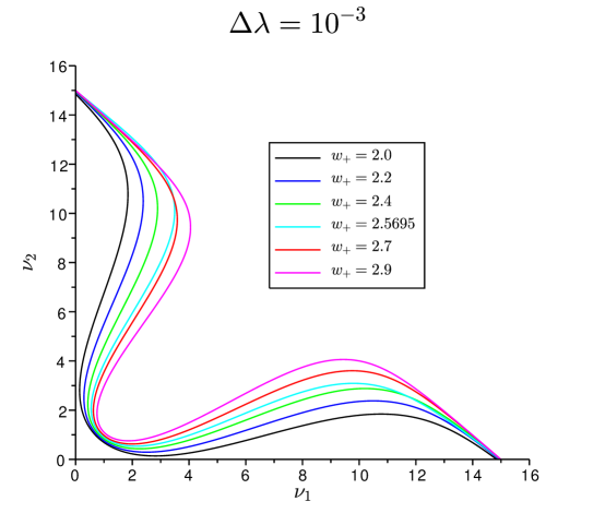
where $\epsilon$ is a small parameter. Assuming that the scaling ratio is zero, $\epsilon=0$, we find the implicit relation $f(x,y)=0$ that determines the approximated slow manifold $x^{*}(y)$. In Figure 3, we plot the curves $x^{*}(y)$ for different values of $\omega_{+}$ with $\Delta\lambda=10^{-3}$. We remark that this restricts the validity of this particular example since these curves exit the set of positive values for the rate variables. This comes from the fact that there are some trajectories of the dynamical system without noise leading to negative values for the rate variables. In this example the approximated curves lie on the positive quadrant for $w_{+}\geq 1.9$ approximately.

Figure 2: Change of variables. Position of the new coordinate system $(x,y)$ with respect to the initial one $(\nu_{1},\nu_{2})$. The origin is taken at the central equilibrium point $S_{0}$ which may stable or unstable accordingly to the value of $w_{+}$. $S_{1}$ and $S_{2}$ are two others equilibrium points. The dashed line represents the slow manifold on which the reduced dynamics takes place, and it contains all the equilibrium points of the system.

Figure 3: Slow manifold. Variation of the approximated slow manifold represented on the $(\nu_{1},\nu_{2})$ plane for $w_{+}=2.0,\ldots,2.9$ and for the biased case $\Delta\lambda=10^{-3}$. For $w_{+}<1.9$ the slow manifold crosses the coordinate axes for small values of $\nu_{1}$ and $\nu_{2}$, becoming negative. The reduction theory is valid only for ranges of $w_{+}>1.9$.

Once we have found the slow manifold approximation $x^{*}(y)$, we can restrict the dynamics in (1) to a single effective Langevin equation. This equation is determined by a potential $G(y)$ obtained from the evaluation of the dynamics over the slow manifold approximation, leading to

$${dy}=g\left(x^{*}(y),y\right){dt}+\beta_{y}\,dW_{t}^{2}\,,$$

with $\beta_{y}$ properly obtained in terms of $\beta$ via the change of variables. The effective potential is determined by the relation $\partial_{y}G(y)=-g(x^{*}(y),y)$. The 1D effective computed potential $G(y)$ for the biased case ($\Delta\lambda=10^{-3}$) with respect to the slow variable $y$ is plotted in Figure 4 for $w_{+}=2.0,\ldots,2.9$ (left), together with a zoom at the spontaneous state (right). We note that increasing $w_{+}$ beyond the second bifurcation point, the spontaneous state pass from local minimum to local maximum. We remind that the effective potential $G(y)$ is given by formula (8) based on the approximated slow manifolds computed in Figure 3.

Figure 4: The 1D potential. Variation of the approximated 1D potential traced along the $y$ variable, varying $w_{+}=2.0,\ldots,2.9$ and for the biased case $\Delta\lambda=10^{-3}$ (left). A zoom around the spontaneous state (right). Increasing $w_{+}$, the central equilibrium point passes from a minima to a maxima.

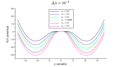
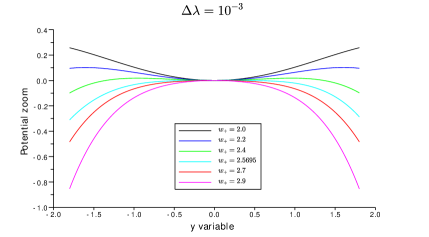
The 1D effective computed potentials $G(y)$ both for the unbiased $\Delta\lambda=0$ and the biased case $\Delta\lambda=10^{-4},10^{-3}$ with respect to the slow variable $y$ are plotted in Figure 5 for the three values of $w_{+}$ close to the second bifurcation point ($w_{+}=2.5685$, $w_{+}=2.5695$, $w_{+}=2.5705$). We note the asymmetry of the effective potential $G(y)$ when increasing the bias $\Delta\lambda$ and the change in the nature of the spontaneous state when increasing the excitatory coefficient $w_{+}$.

Figure 5: Potential at the bifurcation parameter $w_{+}=2.5696$. Top left: $\Delta\lambda=0$, top right: zoom for $\Delta\lambda=0$ around the spontaneous state, middle left: $\Delta\lambda=10^{-4}$, bottom right: zoom for $\Delta\lambda=10^{-4}$ around the spontaneous state, bottom left: $\Delta\lambda=10^{-3}$, bottom right: zoom for $\Delta\lambda=10^{-3}$ around the spontaneous state. For large bias $\Delta\lambda$ the potential becomes asymmetric, and for $\Delta\lambda=10^{-3}$ the spontaneous state changes its nature from a minima to a maxima.

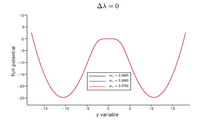
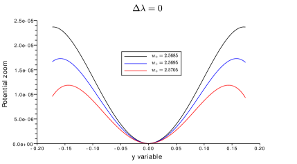
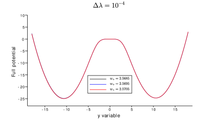
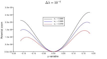
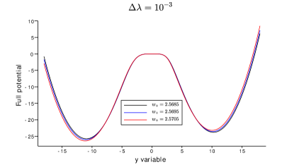
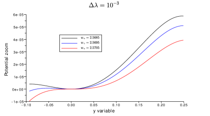
This 1D effective potential can be considered as a good approximation of the equilibrium state of the 2D Fokker-Planck equation (associated to the system (1)) projected on the 1D-slow manifold which is parameterized by the slow variable $y$, see Figure 3. We note that $y>0$ is pointing toward $S_{1}$ while $y<0$ is pointing toward $S_{2}$, see Figure 2. Therefore, the top left (respectively low right) well whose minimum is attained at the stable decision state $S_{1}$ (respectively $S_{2}$) in the 2D $\nu$-plane in Figure 2 corresponds to the right (respectively left) well in Figure 5.

In Figure 6, we have computed the marginals along $y$ of the 2D numerical computations of the Fokker-Planck dynamics for $t=200\ ms$, compared with the solution of the 1D reduction Fokker-Planck evolution equation (7) at $t=200\ ms$. We observe the errors committed by the 1D reductions and we also observe that the slow-fast behavior is also present in the 1D reduced Fokker-Planck equation. However, since the one dimensional reduction is easily solved by numerical methods, then we can achieve much larger computational times and compute explicitly the approximated stationary state.

Figure 6: Distribution function comparison along $y$. The computed marginals of the 2D problem (blue line) at time $t=200\ ms$ and the corresponding solution of the 1D reduced problem (black line) at the same time show a good agreement. In this test we have chosen the bifurcation parameter $w_{+}=2.45$, the standard deviation $\beta=0.3$ and the bias $\Delta\lambda$ takes the values $0,10^{-4}$ and $10^{-3}$.

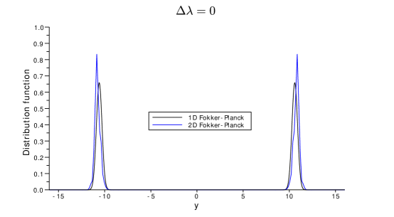
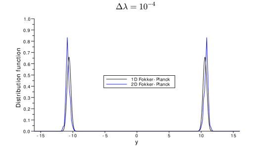
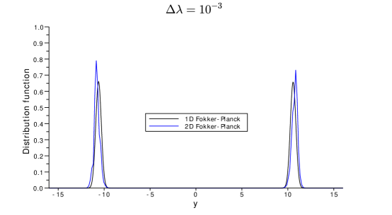
Concerning the comparison between the numerical solutions of the 2D complete Fokker-Planck and those of the 1D reduction, we refer the reader to [13]. We just note here that since the standard deviation is rather small ($\beta=3\cdot 10^{-3}$), the stable states tends to be Dirac masses and the computational costs are unbearable to compute 2D solutions approaching the steady state. Note also that the 1D Fokker-Planck reduction can be solved numerically applying an implicit in time scheme, drastically reducing computational time costs.

Bifurcation: Reaction Time and Performance

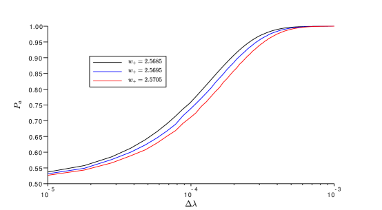
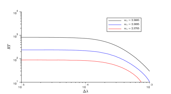
Finally, once the 1D reduction is validated by the above arguments, the biologically interesting quantities to compute are the performance $P_{a}$ and the reaction times $RT$. The first one corresponds to the ratio of good answers at equilibrium, and the second one to the smallest time needed to give an answer, no matter wether it is good or wrong. The computations of the reaction time $RT$ and performances $P_{a}$ use the formulas in the supplementary material in [10], which hold locally around the spontaneous point and are based on the knowledge of the effective potential $G(y)$.

In Figure 7 we plot the performance $P_{a}$ and reaction time $RT$ for $\beta=3\cdot 10^{-3}$ as a functions of $\Delta\lambda$ and $w_{+}$. They are computed for the decision state with higher probability, the one for negative values of the $y$-variable in Figure 5, and over an interval $[a^{-},a^{+}]$ where $a^{-}$ and $a^{+}$ correspond to the $y$-coordinates to the left and right of the spontaneous state for which $G(y)$ has a maximum. We observe the same qualitative behavior as in the comparisons with experimental data performed in [10]. As the bias increases, the potential gets tilted towards the preferred decision state, and thus the performance of the solution gets higher. Accordingly, the reaction time decreases as the bias increases.

Figure 7: Performance and Reaction Times. Top: the performances ($P_{a}$) computed for three values of the bifurcation parameter $w_{+}$ close to the one of the spontaneous state and as a function of the bias $\Delta\lambda$. When $w_{+}$ increases, the performance decreases, and it converges to $1$ for large values of the bias $\Delta\lambda$. Bottom: the reaction times ($RT$) computed for three values of the bifurcation parameter $w_{+}$ close to the one of the spontaneous state and as a function of the bias $\Delta\lambda$. When $w_{+}$ increases, the reaction time decreases. In both pictures the standard deviation is $\beta=3\cdot 10^{-3}$. These behaviors are in agreement with previous results and experimental data.

Discussion

Here, we have reinforced the link between the underlying physiology and the observed behavioral response in decision-making tasks by developing a new strategy for the 1D reduction of the dynamics of the neuronal circuit. In this way we have derived from the underlying detailed neuronal dynamics a ”nonlinear” diffusion model valid for a wide range of the bifurcation parameter. We observe how our method recovers the reduced one dimensional dynamics proposed by Roxin and Ledberg in [10] close to the bifurcation point since we keep the same qualitative behavior in terms of performance and reaction times. We have also shown that our reconstructed effective potential leads to a good approximation of the stationary state of the two dimensional dynamics projected on the slow manifold. This reduction allows for efficient computations of the dynamics as soon as the approximated slow manifold is well-defined.

Materials and Methods

In this section, we give more details of the 1D reduction of system (1) presented above. Preliminary results of this strategy were previously reported in [13] in the easier case of the supercritical Hopf bifurcation. The slow-fast behavior of the system (1) with no noise, i.e. $\beta=0$, can be characterized by the fact that the jacobian of the linearized system at the unstable critical point $S_{0}=(\nu_{1}^{*},\nu_{2}^{*})^{T}$ has a large condition number. More precisely, we write the deterministic part of the dynamical system (1) as $\dot{\nu}=F(\nu)$, where $\nu=(\nu_{1},\nu_{2})^{T}$ is the rate vector and $F(\nu)=-\nu+\Phi(\Lambda+W\nu)$ is the drift. The linearized jacobian matrix at any equilibrium point is given by:

$$J_{F}(z_{1},z_{2})=\left(\begin{array}[]{cc}-1+w_{11}\varphi^{\prime}(z_{1})&w_{12}\varphi^{\prime}(z_{1})\\ w_{21}\varphi^{\prime}(z_{2})&-1+w_{22}\varphi^{\prime}(z_{2})\end{array}\right),$$ (2)

where we have denoted by $z_{i}$ the values $z_{i}:=\lambda_{i}+w_{i1}\nu_{1}+w_{i2}\nu_{2}$. Since $S_{0}$ is a hyperbolic fixed point (saddle point), the jacobian $J_{F}(S_{0})$ has two real eigenvalues, $\mu_{1}$ and $\mu_{2}$ of opposite signs. Let us denote by $\mu_{1}$ the (large in magnitude) negative eigenvalue and by $\mu_{2}$ the (small) positive eigenvalue of $J_{F}(S_{0})$. The small parameter $\varepsilon<<1$ responsible for the slow-fast behavior is determined by the ratio

$$\varepsilon=-\mu_{2}/\mu_{1}.$$

In order to reduce the system we need to introduce new variables based on the linearization of the problem. We will denote by $P$ the matrix containing the normalized eigenvectors of $J_{F}(S_{0})$ and by $P^{-1}$ its inverse matrix. Furthermore, using the Hartman-Gro$\beta$man theorem [14], we know that the solutions of the dynamical system are topologically conjugate with its linearization in the neighborhood of a hyperbolic fixed point. Let us write it as follows

$$J_{F}(S_{0})=PDP^{-1},$$ (3)

where $D=diag(\mu_{1},\mu_{2})$ is the associated diagonal matrix. We can describe the coordinates $\nu$ in the eigenvector basis and centered on the saddle point $S_{0}$ as follows:

$$\nu=S_{0}+PX,$$

which gives the definition for the new variable $X=(x,y)^{T}$, see also figure 2, $X=P^{-1}(\nu-S_{0})$.

In these new coordinates $x$ corresponds to the fast scale while $y$ is the slow varying variable. We can conclude that system (1) reads in the $X$ phase space as $\dot{X}=H(X)$ where $H(X)=(f(x,y),g(x,y))$ is the two dimensional vector defined by $H(X)=P^{-1}F(S_{0}+PX)$, and thus,

$$\begin{cases}\displaystyle\frac{dx}{dt}=f(x,y):=-x-(P^{-1}S_{0})_{1}+\left(P^{-1}\Phi\left(\Lambda+W(S_{0}+PX)\right)\right)_{1}\\[11.38109pt] \displaystyle\frac{dy}{dt}=g(x,y)=-y-(P^{-1}S_{0})_{2}+\left(P^{-1}\Phi\left(\Lambda+W(S_{0}+PX)\right)\right)_{2}\end{cases}\,.$$ (4)

Direct computations gives that $J_{H}(X)=P^{-1}J_{F}(S_{0}+PX)P$, and using (3) and that $X(S_{0})=0$, we obtain that $J_{H}(0)=D$. We can choose a new time scale for the fast variable $\tau=\varepsilon t$ in such a way that for $t\simeq 1$, then $\tau\simeq\varepsilon^{-1}$. Then, the fast character of the variable $x$ is clarified and the system reads as

$$\begin{cases}\varepsilon\displaystyle\frac{dx}{d\tau}=f(x,y)\\[11.38109pt] \displaystyle\frac{dy}{dt}=g(x,y)\end{cases}.$$

Our claim is that the curve of equation $f(x,y)=0$ approximates well when $\epsilon\ll 1$ the slow manifold, that is the unstable manifold that joins the spontaneous point $S_{0}$ to the other equilibrium points. We refer the reader to the discussion in [11] on stochastic slow-fast dynamics. Due to the non-linearity of the function $f$ in (4), we cannot expect an explicit formula for the solution of this equation. Nevertheless, since $\partial_{x}f(0,0)\neq 0$, the resolution in the neighborhood of the unstable equilibrium point $(0,0)$ is insured by the implicit function theorem. Hence we can define a curve:

$$x=x^{*}(y),$$ (5)

such that $f\left(x^{*}(y),y\right)=0$ in a neighborhood of $(0,0)$. We note also that, by construction the approximated slow manifold $S_{0}+P\left(x^{*}(y),y\right)^{T}$, implicitly defined by (5), intersects the exact slow manifold at all equilibrium points, i.e. where both $f$ and $g$ vanishes. Finally, we can conclude the slow-fast ansatz, replacing the complete dynamics by the reduced dynamics on the approximated slow manifold, and obtain the reduced one dimensional differential equation:

$$\dot{y}=g\left(x^{*}(y),y\right).$$

A similar treatment can be done in the presence of the noise terms. By changing variables from $\nu$ to $X$ and since the new variables $x$ and $y$ are linear combination of $\nu_{1}$ and $\nu_{2}$, then it is standard to check

$$\begin{cases}{dx}=f(x,y){dt}+\beta\sqrt{a_{11}^{2}+a_{12}^{2}}\,dW_{t}^{1}\\[8.53581pt] {dy}=g(x,y){dt}+\beta\sqrt{a_{21}^{2}+a_{22}^{2}}\,dW_{t}^{2}\end{cases}\,,$$

where $(a_{ij})$ are the elements of the matrix $P^{-1}$ and $W_{t}^{i}$ are two independent normalized white noise. Arguing as in the deterministic case, we can choose a fast time scale for the variable $x$ and we note that the noise term also changes since $\sqrt{\varepsilon}dW_{t}^{1}=dW_{\tau}^{1}$ and $\varepsilon dt=d\tau$. Therefore, we can deduce again that the reduced one dimensional model must read:

$${dy}=g\left(x^{*}(y),y\right){dt}+\beta_{y}\,dW_{t}^{2},$$ (6)

with $\beta_{y}=\beta\sqrt{a_{21}^{2}+a_{22}^{2}}$.

Finally, we can consider the Fokker-Planck or forward Kolmogorov equation associated to the 1D stochastic differential equation (6). This gives the reduced dynamics for the probability density $q(t,y)$ of finding neurons with rate determined by the rate $y\in[-y_{m},+y_{m}]$ over the approximated slow manifold $S_{0}+P\left(x^{*}(y),y\right)^{T}$, for $t\geq 0$. Actually, it must obey to the following 1D Fokker-Planck equation:

$$\partial_{t}q+\partial_{y}\left(g\left(x^{*}(y),y\right)q-\frac{1}{2}\beta_{y}^{2}\partial_{y}q\right)=0,$$ (7)

with no-flux boundary conditions on $y=\pm y_{m}$: $g\left(x^{*}(y),y\right)q-\frac{1}{2}\beta_{y}^{2}\partial_{y}q=0$, see [15] and [13]. The 1D Fokker-Planck dynamics (7) are given for large times by the stationary solution given by the invariant measure for the stochastic differential equation (6). We can easily find it by defining the associated potential $G(y)$ being the antiderivative of the flux term $g\left(x^{*}(y),y\right)$. In other words, we can always define the potential function:

$$G(y)=-\int_{0}^{y}g\left(x^{*}(z),z\right)dz.$$ (8)

Then, the stationary probability density of the 1D Fokker-Planck dynamics (7) is given by

$$q_{s}(y)=\frac{1}{Z}\exp\left(-2G(y)/\beta_{y}^{2}\right)\,,$$

where $Z$ is the normalization constant. As explained also in [16], this stationary solutions are the asymptotic equilibrium states for the solution of the Fokker-Planck equation. In other words, letting time going to infinity, the solution $q(t,y)$ to (7) must converge to $q_{s}(y)$. We have shown in [16] that the decay to equilibrium for the two dimensional problem was exponential. This rate of convergence is also true for the 1D reduction since the potential is a small perturbation of convex potentials, see the well-know results in [17, 18]. We also recall that we are interested in the long time behavior of the solutions and that the convergence in the slow manifold given by the variable $y$ is slow. Hence it is relevant to have a direct computation of their asymptotic behavior without need to solve the whole 1D or 2D Fokker-Planck equation.

We also remind that the solution of the system (1) is related to the 2D Fokker-Planck or forward Kolmogorov equation:

$$\partial_{t}p+\nabla\cdot\left(F\,p-{\frac{\beta^{2}}{2}}\nabla p\right)=0$$ (9)

with boundary conditions $\left(F\,p-{\frac{\beta^{2}}{2}}\nabla p\right)\cdot n=0$ on the boundary of the domain $[0,\nu_{m}]^{2}$, see [15]. Let us remark that, once we know the stationary state of the 1D reduced Fokker-Planck equation (7), we can approximate the long-time dynamics of all quantities of interest related to the system (1) and the 2D Fokker-Planck (9). More precisely, as $\varepsilon\to 0$, $p$ approaches a concentrated density along the the curve $\nu(y)=S_{0}+P(x^{*}(y),y)^{T}$. Then, for any test function $\Psi=\Psi((\nu_{1},\nu_{2})^{T})$, the moment $M_{\Psi}$ of the stationary probability distribution function $p_{s}(\nu_{1},\nu_{2})$ as $\varepsilon\to 0$ can be approximated by

$$M_{\Psi}=\int_{\Omega}\Psi(\nu)\,p_{s}\,d\nu_{1}d\nu_{2}\simeq\int\Psi\left(S_{0}+P\left(x^{*}(y),y\right)^{T}\right)\,q_{s}(y)\,dy\,.$$

This formulae can be used to compute either classical moments of $p_{s}$ or marginals.

References

- 1. Ratcliff R, Smith P (2004) A comparison of sequential sampling sampling models for two-choice reaction time. Psychol Rev 111: 333 -367.
- 2. Romo R, Salinas E (2001) Touch and go: Decision-making mechanisms in somatosensation. Annu Rev Neurosci 24: 107 -137.
- 3. Romo R, Salinas E (2003) Flutter discrimination: neural codes, perception, memory and decision-making. Nature Reviews Neuroscience 4: 203- 218.
- 4. Shadlen M, Newsome W (2001) Neural basis of a perceptual decision in the parietal cortex (area lip) of the rhesus monkey. J Neurophysiol 86: 1916- 1936.
- 5. Roitman J, Shadlen M (2002) Response of neurons in the lateral intraparietal area during a combined visual discrimination reaction time task. J Neurosci 22: 9475 -9489.
- 6. Huk A, Shadlen M (2005) Neural activity in macaque parietal cortex reflects temporal integration of visual motion signals during perceptual decision making. J Neurosci 25: 10420- 10436.
- 7. Wang X (2002) Probabilistic decision making by slow reverberation in cortical circuits. Neuron 36: 955 -968.
- 8. Wong K, Wang X (2006) A recurrent network mechanism of time integration in perceptual decisions. J Neurosci 26: 1314 -1328.
- 9. Lo C, Wang X (2006) Cortico-basal ganglia circuit mechanism for a decision threshold in reaction time tasks. Nat Neurosci 9: 956 -963.
- 10. Roxin A, Ledberg A (2008) Neurobiological models of two-choice decision making can be reduced to a one-dimensional nonlinear diffusion equation. PLoS Computational Biology 4: 43–100.
- 11. Berglund N, Gentz B (2005) Noise-induced phenomena in slow-fast dynamical systems. a sample-paths approach. Springer, Probability and its Applications .
- 12. Deco G, Martí D (2007) Deterministic analysis of stochastic bifurcations in multi-stable neurodynamical systems. Biol Cybern 96: 487–496.
- 13. Carrillo J, Cordier S, Mancini S (2013) One dimensional Fokker-Planck reduced dynamics of decision making models in computational neuroscience. Comm Math Sci 11: 523- 540.
- 14. Hartman P (1960) A lemma in the theory of structural stability of differential equations. Proc Amer Math Soc 11: 610–620.
- 15. CW G (1985) Handbook of stochastic methods for physics, chemistry and the natural sciences. Springer .
- 16. Carrillo J, Cordier S, S M (2011) A decision-making Fokker-Planck model in computational neuroscience. J Math Biol 63: 801–830.
- 17. Holley R, Stroock D (1987) Logarithmic Sobolev inequalities and stochastic Ising models. J Statist Phys 46: 1159–1194.
- 18. Arnold A, Markowich P, Toscani G, Unterreiter A (2001) On convex Sobolev inequalities and the rate of convergence to equilibrium for Fokker-Planck type equations. Comm Partial Differential Equations 26: 43–100.