Structure and evolution of high-mass stellar mergers

Abstract

In young dense clusters repeated collisions between massive stars may lead to the formation of a very massive star (above $100\,\mbox{${\rm M}_{\odot}$}$). In the past the study of the long-term evolution of merger remnants has mostly focussed on collisions between low-mass stars (up to about $2\,\mbox{${\rm M}_{\odot}$}$) in the context of blue-straggler formation. The evolution of collision products of more massive stars has not been as thoroughly investigated. In this paper we study the long-term evolution of a number of stellar mergers formed by the head-on collision of a primary star with a mass of $5$–$40$ ${\rm M}_{\odot}$ with a lower mass star at three points in its evolution in order to better understand their evolution.

We use smooth particle hydrodynamics (SPH) calculations to model the collision between the stars. The outcome of this calculation is reduced to one dimension and imported into a stellar evolution code. We follow the subsequent evolution of the collision product through the main sequence at least until the onset of helium burning.

We find that little hydrogen is mixed into the core of the collision products, in agreement with previous studies of collisions between low-mass stars. For collisions involving evolved stars we find that during the merger the surface nitrogen abundance can be strongly enhanced. The evolution of most of the collision products proceeds analogously to that of normal stars with the same mass, but with a larger radius and luminosity. However, the evolution of collision products that form with a hydrogen depleted core is markedly different from that of normal stars with the same mass. They undergo a long-lived period of hydrogen shell burning close to the main-sequence band in the Hertzsprung-Russell diagram and spend the initial part of core helium burning as compact blue supergiants.

1 Introduction

Dense stellar systems, such as the cores of star clusters or galactic nuclei, are crowded places where stars frequently interact with each other. In globular clusters, close two-body encounters may form binaries (Hut & Verbunt, 1983); furthermore, two-body encounters can be close enough that two stars can come into physical contact which can lead to a merger (Hills & Day, 1976). Galactic nuclei, where stellar densities reach values in excess of millions of stars per cubic parsec, also harbour stellar collisions. It therefore appears that stellar mergers are natural events in dense stellar systems and this has been demonstrated by several $N$-body simulations (Portegies Zwart et al., 1999; Hurley et al., 2001; Portegies Zwart et al., 2004).

Stellar mergers provide a formation channel for non-canonical stars that cannot be otherwise explained by the standard theory of star formation and evolution, such as blue stragglers that are observed in both open and globular clusters (Sandage, 1953; Johnson & Sandage, 1955; Hills & Day, 1976; Ahumada & Lapasset, 1995; Piotto et al., 2004; Ahumada & Lapasset, 2007). In a young star cluster stellar mergers might be responsible for the formation of massive stars such as the Pistol Star in the Quintuplet Cluster (Figer et al., 1998). Other massive stars, such as Sher $25$ in the massive Galactic cluster NGC 3603, may have been formed via binary mergers and mergers may contribute significantly to the observed population of (rotating) massive stars (Sana et al., 2012; de Mink et al., 2013). Along with the single merger events, some star clusters, such as the Arches close to Galactic centre or R136 in the Large Magellanic Cloud, are dense enough that runaway stellar mergers can occur (Portegies Zwart et al., 2004).

Simulating stellar collisions has attracted considerable attention in the past decade, mostly focussing on globular clusters with the aim of explaining the formation of blue stragglers. Blue stragglers can be formed by stellar collisions or by mass transfer in binary systems. Either of these mechanisms can dominate in one particular cluster, or in different regions of the same cluster (Davies et al., 2004). $N$-body and Monte-Carlo simulations of clusters show that both formation channels are necessary to reproduce the observed blue straggler population (Hurley et al., 2001, 2005; Chatterjee et al., 2013). Nevertheless, there are still many uncertainties regarding blue straggler formation (Leigh et al., 2007, 2011, 2013; Sills et al., 2013).

Dense stellar systems that are abundant in young massive stars, such as the cores of young dense star clusters, are also a natural environment for stellar mergers (Portegies Zwart et al., 1999; Gaburov et al., 2008a). In contrast to globular clusters, the colliding stars have masses that are much larger than the average stellar mass of their environment. If the cluster is dense enough the same star may experience repeated collisions in a so-called ‘merger runaway’ (Portegies Zwart et al., 1999). Such a merger runaway is triggered by the gravo-thermal collapse of the cluster core (Bettwieser & Sugimoto, 1984) and can continue until the target star leaves the main sequence (Portegies Zwart et al., 1999). Only recently have researchers begun to focus their attention on collisions between more massive stars (Freitag & Benz, 2005; Dale & Davies, 2006; Suzuki et al., 2007; Gaburov et al., 2008b; Antonini et al., 2011). These studies were focused either on global properties, such as mass loss, or on the internal structure of collision products; yet very little is known about the evolution of such objects. In earlier work (Glebbeek et al., 2009) we have explored the impact of mass loss on the evolution of the merger runaway. Here we focus on the structure and evolution of single merger products.

In this paper we attempt to improve our understanding by systematically carrying out collision simulations between massive main-sequence stars and studying their further evolution. The aim of this work is to understand the evolution of merger products formed by the merger of two ordinary massive main-sequence stars as a function of stellar ages and masses. This paper is structured as follows. In Section 2 we present the methods we use to carry out this research, in Section 3 we describe the initial conditions for our simulations and in Section 4 we present our results. A discussion of these results and our conclusions are presented in Section 5.

2 Methods

2.1 Hydrodynamic simulations

We use smoothed particle hydrodynamics (SPH) to model stellar collisions. The full details of the SPH method are described in a number of review papers, for instance Monaghan (2005) or Rosswog (2009). We repeat the main points here. SPH is a fully Lagrangian method, which means that it easily adapts to any geometrical configuration without some of the problems in finite-difference methods, such as artefacts due to the choice of coordinate system or numerical diffusion. In addition, the conserved fluid quantities, such as composition, are trivially advected. The largest drawback of SPH, however, is that low density regions are poorly resolved. However, stellar interiors, which contain nearly all the stellar mass, are dense enough for SPH to provide sufficient resolution to capture fine details, such as the density and mean molecular weight gradients across the boundary of a stellar core; for example, in Figure 1 we show the structure of a 20 ${\rm M}_{\odot}$ star at the end of the main-sequence phase. Despite the fact that roughly 30% of the stellar radius is unresolved, this region contributes less than 1% of the stellar mass, so that the internal structure is well resolved.

The simulations that are presented in this paper are carried out by means of a modified version of the GADGET2 code (Springel, 2005). In particular, we have modified the equation of state to include radiation pressure. The modifications are minimal and require only changes in the equation of state and the equation for shock heating. The shock heating term becomes

$$\frac{\,\mathrm{d}A}{\,\mathrm{d}t}=\frac{2}{3}\frac{\rho}{P\beta}A\frac{\,\mathrm{d}Q}{\,\mathrm{d}t}.$$ (1)

Here $dQ/dt$ is the SPH shock heating term which we have not modified, $A(m)$ is the entropic variable (see section 4.2) and $\beta$ is the ratio of gas pressure to total pressure.

 

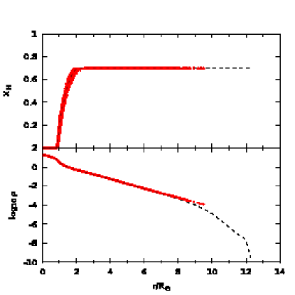
Figure 1: Structure of the 20 ${\rm M}_{\odot}$ primary at the end of the main sequence. The upper panel shows the hydrogen abundance and the lower panel shows the density (in g/cm³), both as a function of the enclosed radius. Dots indicate individual SPH particles (155k, but only 1 in 10 is plotted), the dashed line shows the one dimensional stellar evolution model.

2.2 The stellar evolution code

We use the stellar evolution code originally developed by Eggleton (1971) and later updated by others (e.g. Pols et al., 1995; Glebbeek et al., 2008), hereafter STARS. The STARS code solves the equations of stellar structure and the nuclear energy generation rate simultaneously on an adaptive non-Lagrangian non-Eulerian (“Eggletonian”) grid (Stancliffe, 2006). Chemical mixing due to convection is treated as a diffusion process (Böhm-Vitense, 1958; Eggleton, 1972), as is thermohaline convection (Kippenhahn et al., 1980; Stancliffe et al., 2007). Our mixing coefficient for thermohaline convection is based on the expression of (Kippenhahn et al., 1980),

$$D_{\mathrm{thm}}=C\frac{16acT^{3}}{c_{P}\rho^{2}\kappa}\frac{\nabla_{\mu}}{\nabla_{\mathrm{ad}}-\nabla}.$$ (2)

The efficiency parameter $C$ is set to $100$ to reproduce the efficiency calibration by Charbonnel & Zahn (2007).

Our reaction rates are the recommended rates from Angulo et al. (1999), with the exception of ${}^{14}\mathrm{N}(\mathrm{p},\gamma)^{15}\mathrm{O}$, for which we use the recommended rate from Herwig et al. (2006) and Formicola et al. (2004). Opacities are from Iglesias & Rogers (1996), with molecular opacities from Ferguson et al. (2005) and conductive opacities from Cassisi et al. (2007). Mass loss by stellar winds is included using the prescription of Vink et al. (2000, 2001) or de Jager et al. (1988) at cooler temperatures.

The conversion of the collision output to stellar evolution input is done using the method described by Glebbeek et al. (2008). Once a suitable input model has been constructed we follow the subsequent evolution of the merger remnant.

3 Initial conditions

The aim of this work is to understand the structure and the evolution of massive stellar collision products. The structure of the collision product is influenced by the masses and composition of the colliding (parent) stars as well as the parameters of the collision. We therefore need to span a section of the parameter space that encompasses a variety of initial conditions for the geometry of the collisions and the masses and ages of the parent stars. In this study we focus on head-on collisions, ignoring the complications associated with rotation in the merger product (e.g. Sills et al., 2005) in order to focus on the influence of the parent star masses and ages. We consider only collisions where the total orbital energy is zero (‘parabolic’ collisions). This limitation can be justified by the fact that the velocity dispersion in young star clusters is much smaller than the escape velocity from the stellar surface and therefore has little influence on the structure of the merger remnant.

3.1 Masses and ages of the parent stars

Figure 2: Hertzsprung-Russell diagram of our primary stars, with (from top to bottom) masses of 40, 20, 10 and 5 ${\rm M}_{\odot}$, showing the points chosen for our collisions. The HAMS by $\bullet$ and TAMS and CHEX by $\blacktriangle$ and $\blacktriangledown$ respectively. For completeness, the ZAMS is indicated by $\blacksquare$.

We systematically study collisions between massive stars of different masses and ages, but with the same initial composition. We vary the mass of the primary star $M_{1}$ and the mass ratio $q=M_{2}/M_{1}$ between the secondary and the primary.

We choose the ages of the parent stars based on the evolution stage of the primary, as illustrated in Figure 2: halfway through the main-sequence lifetime (HAMS), at the terminal-age main-sequence (TAMS) or at core hydrogen exhaustion (CHEX). Here TAMS refers to the reddest point before the hook at core hydrogen exhaustion. This normally corresponds to the moment where the star has $3$–$4\%$ by mass of hydrogen left in the core, but in some of our TAMS models the central hydrogen abundance is smaller ($1$–$0.1$%). The CHEX stage is shortly after this stage, at the bluest point after the TAMS stage but before the Hertzsprung gap. This corresponds to actual core hydrogen exhaustion, or a hydrogen abundance of about $0.01\%$ in the core depending on the mass of the star. The masses of the primaries are chosen to be $5$, $10$, $20$ and $40$ ${\rm M}_{\odot}$, whereas the masses of the secondary star are chosen according to the mass ratio $q$, which takes the values $0.1$, $0.4$, $0.7$ and $1.0$. This was done to get a reasonable coverage between equal masses and extreme mass ratios. For CHEX stars we choose $q=0.99$ rather than $1.0$, which roughly corresponds to a collision between a CHEX and a TAMS star. To simplify the notation later we will refer to a collision between a 10 ${\rm M}_{\odot}$ TAMS star and a 1 ${\rm M}_{\odot}$ star (say) as ‘TAMS 10+1’.

Table 1: This table presents an overview of the simulations presented in this work. The first and second columns show the mass of the primary and the secondary star respectively, the third column shows the mass ratio. The fifth and sixth columns display the number of SPH particles used in each of the stars, and the last column indicates the evolutionary stage of the primary. In most of the simulations we use $262\mathrm{k}$ particles. One of the CHEX models is also simulated with higher resolution ($560\mathrm{k}$ particles) to verify that the lower resolution simulations capture the essential details. All stellar models are of solar metallicity ($Z=0.02$).

$M_{1}$ [${\rm M}_{\odot}$]	$M_{2}$ [${\rm M}_{\odot}$]	$q$	$N_{1}/1000$	$N_{2}/1000$	Age
40	40	1.0	131	131	TAMS, HAMS
40	39.6	0.99	132	130	CHEX
40	28	0.7	155	107	CHEX, TAMS, HAMS
40	16	0.4	400	160	CHEX
40	16	0.4	187	75	CHEX, TAMS
40	4	0.1	239	23	CHEX, TAMS, HAMS
20	20	1.0	131	131	TAMS
20	19.8	0.99	132	130	CHEX
20	14	0.7	155	107	CHEX, TAMS, HAMS
20	8	0.4	187	75	CHEX, TAMS
20	2	0.1	239	23	CHEX, TAMS, HAMS
10	10	1.0	131	131	TAMS
10	9.9	0.99	132	130	CHEX
10	7	0.7	155	107	CHEX, TAMS, HAMS
10	4	0.4	187	75	CHEX, TAMS
10	1	0.1	239	23	CHEX, TAMS, HAMS
5	5	1.0	131	131	TAMS
5	4.95	0.99	132	130	CHEX
5	3.5	0.7	155	107	CHEX, TAMS, HAMS
5	2	0.4	187	75	CHEX, TAMS
5	0.5	0.1	239	23	CHEX, TAMS, HAMS

3.2 Stellar models and set-up of simulations

The full set of simulations that we carried out is presented in Table 1. Most of the simulations use $262\mathrm{k}$ equal mass SPH particles. This number was chosen such that we are able to accurately resolve the internal structure of the collision product (Sills et al., 2002; Gaburov et al., 2008b).

We prepare our 3D SPH models based on 1D stellar evolution models calculated with STARS. Our input models are non-rotating and start with an initial heavy element abundance (metallicity) $Z=0.02$ and a hydrogen abundance $X=0.70$. For each collision we calculate the evolution of the primary from the zero-age main-sequance (ZAMS) until the appropriate age (HAMS, TAMS or CHEX) and then evolve the secondary to the same age as the primary. We use the composition, density and temperature profiles of the 1D models to construct a quasi-hydrostatic equilibrium SPH model.

We use the resulting three-dimensional SPH models to prepare our collision simulations. The parent stars are initially separated by a distance that is equal to twice the sum of their radii and with the velocity of each star computed in such a way that the total orbital energy, angular momentum and velocity of the centre of mass is zero. The stellar velocities are directed towards each other.

3.3 Reduction of three-dimension data

In order to import the results of our collision calculations into the stellar evolution code the three-dimensional data has to be reduced to one dimension and converted into a format that is understandable by the stellar evolution code. A collision between stars is a complex hydrodynamic interaction of self-gravitating fluids, and such interactions do not posses apparent symmetries. Shocks together with turbulent heating result in mixing of the fluid that is intrinsically three-dimensional. However, the structure of a head-on collision product is spherically symmetric once the fluid has settled into hydrostatic equilibrium. This allows us to reduce the three-dimensional data to one dimension by averaging over isobaric surfaces.

The collision calculations do not have sufficient resolution to resolve the outer parts of the envelope near the photosphere, which means that we do not have information about the structure of the envelope at that point. However, for the stellar evolution code the input model needs to satisfy the photospheric boundary condition. Sills et al. (1997) extrapolated the entropy profile and used the condition of hydrostatic equilibrium to reconstruct the outer layers. Because our method to import the stellar evolution models is fully implicit we find it easier to allow the evolution code to simply adjust the unresolved layers in response to the stellar interior (Glebbeek et al., 2008), which is equivalent to assuming that the outer layers are in thermal equilibrium at the start of our evolution calculations. This is a reasonable approximation because the thermal timescale for these layers is short compared to the thermal timescale of the entire star. As noted by Sills et al. (1997), the long term evolution of the collision product is not sensitive to the treatment of the surface layers but the exact shape of the evolution track during the contraction phase is.

4 Results

4.1 Mass loss from the collision

Figure 3: Mass loss from the collisions as a function of the mass ratio $q$. The results from our simluations are indicated by $\bullet$, the prediction of Eq. (3) is shown as $\times$ and the prediction of Eq. (4) is shown with a dashed line.

For central collisions between low mass stars Lombardi et al. (2002) found that the fraction of mass ejected by the collision $\phi$ can be modelled using

$$\phi=C_{1}\frac{q}{(1+q)^{2}}\frac{R_{1,0.86}+R_{2,0.86}}{R_{1,0.5}+R_{2,0.5}}.$$ (3)

Here $R_{n,0.86}$ and $R_{n,0.5}$ are the radii containing 86% and 50% of the mass of parent star $n$ (1 or 2). The constant $C_{1}=0.157$. Glebbeek & Pols (2008) found that for a set of low mass collisions, the mass loss could also be modelled using the simpler prescription

$$\phi=C_{2}\frac{q}{(1+q)^{2}},$$ (4)

with $C_{2}=0.3$. The result from our simulations is shown in Figure 3 along with both of these prescriptions. As can be seen from the figure, Eq. (3) gives a better agreement for extreme mass ratio collisions but underpredicts the mass loss at more equal mass ratios. The simpler prescription Eq. (4) slightly overpredicts the mass loss at low mass ratios but gives a better estimate at more equal masses.

4.2 Structure of the collision products

It was shown by Lombardi et al. (2002) that there is a simple physical mechanism that determines the structure of a collision product, and this provides a quick method to obtain the approximate structure of the collision product as well as to understand the outcome of SPH calculations. The intricate details of shock and turbulent heating cannot be predicted by simple analytical models, but an empirical tabulation of shock heating, which is based on a number of simulations combined with conservation laws, provides an accurate estimate of the degree of shock heating (Lombardi et al., 2002, 2003; Gaburov et al., 2008b).

For a chemically homogeneous star in hydrostatic equilibrium the entropy increases outward. The idea behind the method is to find a function of entropy and composition that increases outward in stars that are not chemically homogeneous. Such a function is $A=P/\rho^{5/3}\exp[8(1-\beta)/3\beta]$ (Gaburov et al., 2008b). We call this function $A(m)$ the buoyancy, since for stable hydrostatic equilibrium the fluid with higher buoyancy should generally be above the fluid with lower buoyancy. It is related to the entropy of the gas and is also known in the literature as the entropic variable. The stability condition is (Gaburov et al., 2008b)

$$\frac{\,\mathrm{d}\log A}{\,\mathrm{d}{m}}>\frac{4}{3}\frac{\frac{5}{3}-\Gamma_{1}}{\Gamma_{1}-\frac{4}{3}}\displaystyle\frac{\,\mathrm{d}\log\mu}{\,\mathrm{d}{m}}.$$ (5)

Here $\mu$ is the mean molecular weight of the fluid element and $\Gamma_{1}=(\partial\log P/\partial\log\rho)_{\mathrm{ad}}$ is the adiabatic index of the element (Clayton, 1983; Kippenhahn & Weigert, 1990) and $m$ is the enclosed mass.

In the case of a monatomic ideal gas ($\Gamma_{1}=5/3$) or a chemically homogeneous fluid (${\rm d}\mu/{\rm d}m=0$) the stability condition simplifies to ${\rm d}A/{\rm d}m>0$. Heating is important because it modifies the entropy in each of the parent stars. Therefore, for proper modelling one needs to take into account the conversion of orbital kinetic energy into heat (Lombardi et al., 2002; Gaburov et al., 2008b).

For collisions between unevolved (ZAMS) stars equation Eq. (5) implies that the core of the lower mass star sinks to the centre of the collision product. For evolved stars the situation is more complicated because stellar evolution decreases $A$ in the core of the primary more quickly than in the core of the secondary, but it is still possible that the core of the secondary retains its identity and sinks to the centre of the collision product. Following the results of Glebbeek & Pols (2008) for collisions between low-mass stars we identify the cases ‘M’, ‘P’ and ‘S’ depending on whether the core of the collision product is a mixture of material from the progenitor stars, or predominantly comes from the primary or the secondary.

Case M

If the buoyancy in the cores of the two progenitor stars is similar, or if the two stars are very close in mass, the material in the core will be a mixture of the material in the cores of the two parent stars. After the collision the hydrogen abundance in the core will be in between the core hydrogen abundances in the progenitor stars. There can be a molecular weight inversion if the material just outside the core predominantly comes from the primary.

Case P

If the primary is sufficiently evolved, the core of the primary becomes the core of the collision product. This does not normally lead to a molecular weight inversion, but it does mean that the collision product has an anomalously small core for a star of its mass. If the core cannot grow, for instance because hydrogen has already been exhausted and there is no nuclear burning, the evolution path of the collision product can be very different from that of a normal star of the same mass, as will be discussed in section 4.3.

Case S

If stellar evolution has not decreased the buoyancy in the primary core sufficiently, the core of the secondary will displace the core of the primary and occupy the centre of the collision product. This can happen at moderate mass ratios if the primary is relatively unevolved, or it can happen at more extreme mass ratios even if the primary is already at the end of the main sequence. In either of these cases the core of the collision product will be hydrogen rich, with a helium rich layer just outside the core.

4.2.1 Half Age Main Sequence

Stars at half of their main-sequence age have converted a notable amount of hydrogen into helium. During the collision, the stellar interior is heated via shock waves, turbulent heating and tidal interactions. The result is that some of the helium-enriched material from the interior is mixed into the outer layers; at the same time, part of the weakly bound outer layers are ejected. The amount of mass loss in these collision is relatively small, as shown in Table 2.

Table 2: Mass lost from HAMS collisions. The first column is the ZAMS mass of the primary star and its mass at the moment of collision in brackets, the second column is the ZAMS mass of the secondary with the mass at the moment of collision given in brackets, the third column is the fractional mass loss as a percentage of the total mass and the last column identifies the collision case (M, P or S, see text).

$M_{1}$ [${\rm M}_{\odot}$]	$M_{2}$ [${\rm M}_{\odot}$]	$M_{\rm lost}$ [%]	Case
40 (39.3)	40 (39.3)	6.2	M
40 (39.3)	28 (27.7)	6.2	M
20 (19.8)	14 (14.0)	6.5	M
10 (9.98)	7 (7.00)	6.8	M
5 (5.00)	3.5 (3.50)	6.9	M
40 (39.3)	4 (4.00)	0.70	S
20 (19.8)	2 (2.00)	0.66	S
10 (9.98)	1 (1.00)	0.81	S
5 (5.00)	0.5 (0.50)	1.3	S

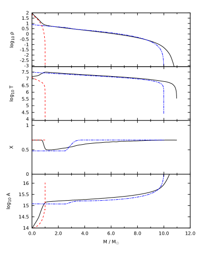
Figure 4: Structure of the HAMS 10+1 merger product. The upper panel shows the density profile as a function of enclosed mass, the second panel from the top presents the temperature profile and the two lowest panels display the hydrogen mass fraction and buoyancy profile as a function of enclosed mass respectively. The dashed line (blue) shows the structure of the secondary and the dash-dotted line (red) shows the structure of the primary.

In Figure 4 we show the structure of the HAMS 10+1 merger product, which is an example of case S that illustrates some of the characteristic features. The $1\,\mbox{${\rm M}_{\odot}$}$ star remains almost completely intact, as can be seen from the hydrogen profile. This results in a molecular weight inversion at the edge of the core at $1\,\mbox{${\rm M}_{\odot}$}$. Because the secondary retains its identity but now finds itself compressed in the interior of a more massive star, the core of the merger product is overdense and overheated compared to a $1\,\mbox{${\rm M}_{\odot}$}$ star. However, the entropy in the core is low compared to the entropy in a ZAMS star of the same mass and composition as the merger product. This results in a steepening of the density profile below $1\,\mbox{${\rm M}_{\odot}$}$ and a temperature inversion, with the maximum temperature occurring at 1 ${\rm M}_{\odot}$.

4.2.2 Terminal-age main sequence star (TAMS)

Table 3: As Table 2 for TAMS collisions.

$M_{1}$ (${\rm M}_{\odot}$)	$M_{2}$ (${\rm M}_{\odot}$)	$M_{\rm lost}$ (%)	Case
40 (36.7)	40 (36.7)	8.3	M
20 (19.4)	20 (19.4)	8.0	M
10 (9.98)	10 (9.98)	8.1	M
5 (5.00)	5.0 (5.00)	8.2	M
40 (36.7)	28 (27.2)	8.0	M
20 (19.4)	14 (13.9)	7.6	P
10 (9.98)	7 (7.00)	7.6	P
5 (5.00)	3.5 (3.5)	7.6	P
40 (36.7)	16 (15.9)	8.6	S
20 (19.4)	8 (8.00)	8.2	S
10 (9.98)	4 (4.00)	7.3	S
5 (5.00)	2 (2.00)	7.5	S
40 (36.7)	4 (4.00)	2.1	S
20 (19.4)	2 (2.00)	1.5	S
10 (9.98)	1 (1.00)	1.4	S
5 (5.00)	0.5 (0.50)	2.2	S

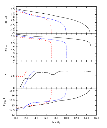
Figure 5: As Figure 4 for the TAMS 10+7 merger product.

Table 4: As Table 2 for CHEX collisions.

$M_{1}$ (${\rm M}_{\odot}$)	$M_{2}$ (${\rm M}_{\odot}$)	$M_{\rm lost}$ (%)	Case
40 (36.7)	39.6 (36.4)	8.0	M
20 (19.4)	19.8 (19.2)	8.0	M
10 (9.98)	9.9 (9.88)	8.0	M
5 (5.00)	4.95 (4.95)	8.1	M
40 (36.7)	28 (27.2)	7.8	M
20 (19.4)	14 (13.9)	7.7	P
10 (9.98)	7 (7.00)	7.7	P
5 (5.00)	3.5 (3.5)	7.7	P
40 (36.7)	16 (15.9)	8.6 (8.8)	S
20 (19.4)	8 (8.00)	8.2	S
10 (9.98)	4 (4.00)	7.8	S
5 (5.00)	2 (2.00)	7.5	M
40 (36.7)	4 (4.00)	2.1	S
20 (19.4)	2 (2.00)	1.5	S
10 (9.98)	1 (1.00)	1.5	S
5 (5.00)	0.5 (0.50)	2.3	S

For TAMS stars the envelope is less strongly bound compared to HAMS stars and therefore a larger fraction of mass is lost, as shown in Table 3. It can be seen that the mass loss fraction is also a decreasing function of the mass ratio $q$. This is because the orbital kinetic energy, which is dissipated into heat and used to eject the material, is proportional to the product of the masses of the parent stars $M_{1}M_{2}=qM_{1}^{2}$.

An example of a case P merger product is the TAMS 10+7 product shown in Figure 5. In this case the core of the primary contained $0.1\%$ by mass of hydrogen at the time of collision and the core of the secondary is unable to displace the core of the primary. The inner $0.5\,\mbox{${\rm M}_{\odot}$}$ of the remnant consists of hydrogen depleted material from the primary, while the material between $0.5\,\mbox{${\rm M}_{\odot}$}$ and $1\,\mbox{${\rm M}_{\odot}$}$ is a mixture of material from the primary and the secondary. The central density and temperature are again higher than in the core of the $10\,\mbox{${\rm M}_{\odot}$}$ primary, but in this case there is no temperature inversion.

4.2.3 Core Hydrogen Exhaustion (CHEX)

Stars that have completely exhausted hydrogen in their cores (CHEX stars) have a similar structure to TAMS stars. Therefore we expect that the structure of the merger products and mass loss are similar to TAMS collisions. Indeed, Table 4 shows that the mass lost in collisions between CHEX stars is quantitatively similar to the mass lost in collisions between TAMS stars.

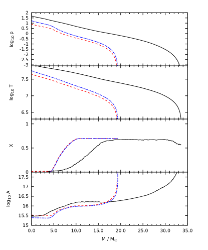
(a) 20 + 19.8

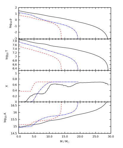
(b) 20 + 14

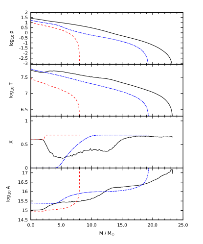
(c) 20 + 8

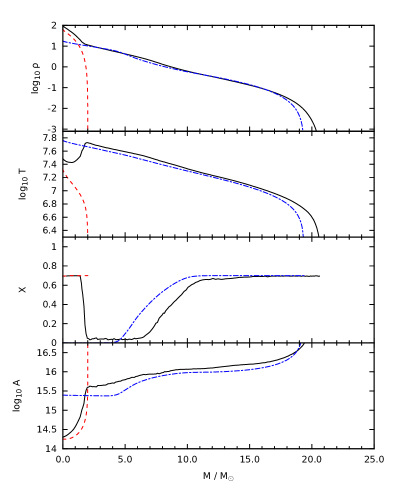
(d) 20 + 2

Figure 6: As Figure 4 for the CHEX collisions with a 20 ${\rm M}_{\odot}$ primary and 19.8 (upper left panel), 14 (upper right panel), 8 (lower left panel) and 2 (lower right panel) ${\rm M}_{\odot}$ secondaries. In all cases the dashed line (red) shows the structure of the secondary and the dash-dotted line (blue) shows the structure of the primary.

In Figure 6 we show the structure of the merger products of which the primary is a 20 ${\rm M}_{\odot}$ CHEX star and the secondary covers a mass range such that the mass ratio $q$ is 0.99 (6(a)), 0.7 (6(b)), 0.4 (6(c)) and 0.1 (6(d)). Each of the three cases occurs in one of these panels. The CHEX 20+19.8 collision is a clear example of case P, while CHEX 20+14 can be considered case M since a notable amount of hydrogen from the secondary has been mixed into the core. Despite this, the material in the core predominantly comes from the primary and is hydrogen poor. The CHEX 20+8 and CHEX 20+2 are both case S, although the differences are quite interesting. In both cases the inner $\sim 2\,\mbox{${\rm M}_{\odot}$}$ consists of hydrogen-rich material from the core of the secondary. In the CHEX 20+2 case, this means the entire star occupies the core of the merger product with a strong enhancement in the helium abundance of the envelope. In the CHEX 20+8 case there is an additional $6\,\mbox{${\rm M}_{\odot}$}$ of hydrogen-rich material that is mixed into the envelope, which dilutes the helium enhancement considerably. As with the HAMS 10+1 merger product, the CHEX 20+2 remnant shows a notable temperature inversion just outside the core and a clear kink in the density profile. No such kink appears in the CHEX 20+8 case, although there is a small temperature inversion. We will return to these features when considering the evolution in section 4.3.1.

4.3 Evolution of the merger remnants

We have calculated the evolution of the merger products listed in Table 1. The results of our evolution calculations are presented in Table 5. A few models are missing from this table: we were unable to follow the evolution of these models for more than a few timesteps before the evolution code broke down. Also missing is the Hertzsprung gap evolution for CHEX 5+0.5, which broke down shortly after the contraction phase.

Table 5: Evolution results for the merger products. The first three columns list the evolutionary stage of the primary (HAMS, ZAMS or CHEX), the mass of the primary $M_{1}$ and the mass of the secondary $M_{2}$ (both in ${\rm M}_{\odot}$). Column four identifies the collision case (M, S or P, see text) and column five gives the total mass of the remnant $M_{\mathrm{rmn}}$ at the beginning of the evolution. Columns six through thirteen give the amount of mass loss in the collision $\Delta M$, the total main sequence lifetimes $\tau_{\mathrm{ms,1}}$ and $\tau_{\mathrm{ms,2}}$ of the progenitor stars, the main sequence lifetime of a star born with the same mass as the merger product $\tau_{\mathrm{ms}}$, the actual main sequence (core hydrogen burning) lifetime $t_{\mathrm{ms}}$ of the merger product, the time $\tau_{\mathrm{HG}}$ spend in the Hertzsprung gap by a star born with the same mass, the time $t_{\mathrm{HG}}$ the merger product spends in this part of the Hertzsprung-Russell diagram and the time $t_{\mathrm{HSB}}$ between the end of core hydrogen burning and central helium ignition (i.e. the length of hydrogen shell burning). All times are given in Myr and masses are in solar units. The final two columns give the helium core mass $M_{\mathrm{He}}$ at the moment of helium ignition and helium core mass $M_{\mathrm{He,ms}}$ in a normal star at helium ignition.

Stage	$M_{1}$	$M_{2}$	Case	$M_{\mathrm{rmn}}$	$\Delta M$	$\tau_{\mathrm{ms,1}}$	$\tau_{\mathrm{ms,2}}$	$\tau_{\mathrm{ms}}$	$t_{\mathrm{ms}}$	$\tau_{\mathrm{HG}}$	$t_{\mathrm{HG}}$	$t_{\mathrm{HSB}}$	$M_{\mathrm{He}}$	$M_{\mathrm{He,ms}}$
HAMS	5	0.5	S	5.43	0.07	82.03	124027	81.92	57.43	0.52	0.52	0.64	0.98	0.94
HAMS	10	1	S	10.86	0.13	19.82	8646	19.87	13.44	0.07	0.07	0.07	2.67	2.53
HAMS	20	2	S	21.43	0.36	7.72	908	7.98	5.25	0.03	0.03	0.02	6.55	6.19
HAMS	40	4	S	41.90	1.40	4.28	141	4.48	2.81	0.01	0.01	0.01	16.78	15.34
HAMS	5	3.5	M	8.00	0.50	82.03	199	35.26	27.38	0.19	0.13	0.15	1.70	1.60
HAMS	10	7	M	16.00	0.99	19.82	38.89	11.17	8.43	0.06	0.04	0.02	4.24	3.91
HAMS	20	14	M	31.76	2.00	7.72	11.85	5.47	3.89	0.02	0.02	0.01	10.98	10.14
HAMS	40	28	M	63.10	3.91	4.28	5.62	3.53	2.36	0.01	0.01	0.01	28.22	26.42
TAMS	5	0.5	S	5.38	0.12	82.03	124027	83.84	22.09	0.52	0.66	0.79	0.92	0.93
TAMS	10	1	S	10.83	0.15	19.82	8646	19.86	4.67	0.08	0.08	0.07	2.43	2.38
TAMS	20	2	S	21.04	0.32	7.72	908	8.14	1.79	0.03	0.03	0.02	6.56	6.04
TAMS	40	4	S	39.85	0.85	4.28	141	4.63	0.78	0.01	0.01	0.01	15.73	14.28
TAMS	5	2	S	6.47	0.53	82.03	908	54.96	27.01	0.32	0.30	0.34	1.29	1.19
TAMS	10	4	S	12.96	1.02	19.82	141	14.92	6.54	0.06	0.05	0.04	3.64	3.02
TAMS	20	8	S	25.16	2.20	7.72	29.75	6.78	2.41	0.02	0.02	0.01	8.62	7.72
TAMS	40	16	S	48.09	4.52	4.28	9.96	4.11	1.18	0.01	0.02	0.01	22.11	18.28
TAMS	5	3.5	P	7.86	0.64	82.03	199	36.40	0.06	0.16	12.00	11.86	1.01	1.57
TAMS	10	7	P	15.70	1.28	19.82	38.89	11.42	0.01	0.06	4.11	3.16	1.49	3.78
TAMS	20	14	M	30.73	2.55	7.72	11.85	5.63	0.01	0.02	2.05	1.96	12.69	9.84
TAMS	40	28	M	58.81	5.09	4.28	5.62	3.68	0.02	0.01	0.00	0.85	30.17	28.47
TAMS	5	5	M	9.18	0.81	82.03	82.03	26.86	0.01	0.11	3.90	0.58	1.11	1.96
TAMS	10	10	M	18.35	1.61	19.82	19.82	9.49	0.02	0.04	2.89	2.87	6.39	4.94
TAMS	20	20	M	35.62	3.11	7.72	7.72	5.00	1.29	0.01	0.01	0.01	13.36	12.23
CHEX	5	0.5	S	5.37	0.13	82.03	124027	84.23	23.28	0.61	0.63	0.77	0.92	0.93
CHEX	10	1	S	10.81	0.17	19.82	8646	20.04	4.63	0.08	0.08	0.07	2.49	2.52
CHEX	20	2	S	21.04	0.32	7.72	908	8.14	1.76	0.03	0.03	0.02	6.49	6.04
CHEX	40	4	S	39.84	0.85	4.28	141	4.63	0.74	0.01	0.06	0.01	15.70	14.22
CHEX	5	2	M	6.47	0.53	82.03	908	54.96	26.04	0.32	0.29	0.34	1.31	1.19
CHEX	10	4	S	12.89	1.09	19.82	141	15.09	6.46	0.06	0.04	0.04	3.54	3.02
CHEX	20	8	S	25.13	2.23	7.72	29.75	6.79	2.34	0.02	0.02	0.02	8.47	7.71
CHEX	40	16	S	48.09	4.52	4.28	9.96	4.08	1.26	0.01	0.01	0.01	22.33	17.73
CHEX	5	3.5	P	7.85	0.65	82.03	199	0.00	0.00	0.00	12.55	11.24	0.98	0.00
CHEX	10	7	P	15.68	1.30	19.82	38.89	11.50	0.00	0.05	4.10	2.14	1.28	3.84
CHEX	20	14	P	30.71	2.57	7.72	11.85	5.63	0.00	0.02	1.94	1.86	12.68	9.85
CHEX	40	28	M	58.89	5.01	4.28	5.62	3.67	0.96	0.01	0.01	0.01	32.30	28.50
CHEX	5	4.95	M	9.14	0.81	82.03	102	23.18	0.00	0.09	2.20	2.05	1.14	2.22
CHEX	5	4.95	M	9.14	0.81	82.03	102	27.07	0.00	0.11	2.20	2.05	1.14	1.95
CHEX	20	19.8	M	35.46	3.08	7.72	8.65	5.02	0.00	0.02	1.43	1.39	16.39	12.16
CHEX	40	39.6	M	67.26	5.82	4.28	4.53	3.41	0.00	0.01	0.00	0.65	39.24	31.34

For completeness Table 5 gives the total remnant mass as well as the collision case. The table also lists the time $t_{\mathrm{ms}}$ that the merger product spends as a core hydrogen burning star and the time $t_{\mathrm{HG}}$ spend in the Hertzsprung gap, between the end of core hydrogen burning (CHEX) and the base of the giant branch. The duration of the hydrogen shell burning phase is given by $t_{\mathrm{HSB}}$. This phase ends with the ignition of helium in the core. Note that with these definitions the evolution in the Hertzsprung gap can include part of the core-helium burning phase, in which case $t_{\mathrm{HG}}>t_{\mathrm{HSB}}$. We discuss this in more detail in section 4.3.2. The table also gives the core mass $M_{\mathrm{He}}$ at helium ignition.

4.3.1 Contraction phase and core hydrogen burning

Figure 7: Evolution track of the HAMS 10+7 merger product in the Hertzsprung-Russel diagram (solid line). The dotted line shows the evolution track of a normal star of the same mass as the merger product.

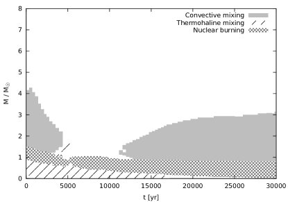
Figure 8: Kippenhahn diagram showing the evolution of the HAMS 10+1 merger product during the contraction phase. Note that initially, hydrogen is burning in a shell outside the core. Thermohaline mixing is responsible for mixing into the central hydrogen rich core while convection mixes the region just above the burning shell.

Figure 9: Evolution track of the HAMS 10+1 merger product in the $\log\rho$–$\log T$ plane. The solid line shows the evolution of the stellar centre while the dash-dotted line shows the evolution of the locus of highest temperature. The starting point of the evolution is indicated by $+\times$. The dotted line shows the transition of hydrogen shell burning to hydrogen core burning. For reference, the dashed line shows the evolution track of a normal star of the same initial mass as the merger product.

The first phase of evolution after the collision is the contraction phase, which progresses similarly to that for low-mass merger products, as studied in a previous paper (Glebbeek et al., 2008) and before by other authors (Sills et al., 1997). The evolution track for the HAMS 10+7 collision shown in Figure 7 shows the typical features for the merger product evolution tracks. During the contraction phase the merger product is inflated and over-luminous. In this example the stellar radius is inflated by a factor of 100 compared to the equilibrium radius, but the star contracts quickly and after only 200 years the radius is only five times the equilibrium radius. The initial radius is sensitive to the assumptions made about the surface layers (as discussed in Section 3.3). Most of the star’s luminosity is provided by the release of thermal energy and the envelope contracts on a thermal timescale. In all our merger products the envelope is enhanced in helium, which means it is brighter than a normal star of the same mass, as we found for low-mass mergers (Glebbeek et al., 2008, 2010; Glebbeek & Pols, 2008).

If the core of the merger product is made up of material from the primary (case P) or is a mixture of material from the progenitor stars (case M), the highest temperature occurs in the centre of the merger product. Because the core is hydrogen rich, hydrogen ignites in the centre. Temperature inversions like the one found in the HAMS 10+1 collision product can result in the formation of a hydrogen burning shell on top of a hydrogen-rich core if the hydrogen abundance in the region of maximum temperature is high enough. During the contraction phase these temperature inversions are removed and the burning front moves inward to the centre of the remnant. At the same time molecular weight inversions in the interior are removed by thermohaline mixing (Kippenhahn et al., 1980).

The evolution of the stellar interior for the HAMS 10+1 merger product (case S) is shown in Figure 8 and Figure 9. As discussed in section 4.2.1 the core of the merger product consists of material from the $1\,\mbox{${\rm M}_{\odot}$}$ secondary star and is overdense. This means that it needs to expand in order to reach thermal equilibrium. Because this requires work against the pressure exerted by the envelope and the expansion is nearly adiabatic the temperature in the core decreases. The highest temperature occurs in a helium rich hydrogen burning shell above the core. Local conditions in the burning shell are close to the prevailing conditions in the core of a normal $11\,\mbox{${\rm M}_{\odot}$}$ star (see the dash-dotted line in Figure 9). The burning shell becomes denser. Because the molecular weight in the burning shell is higher than the molecular weight in the core thermohaline mixing operates, which slowly homogenises the inner part of the star. Figure 8 shows the evolution in a Kippenhahn diagram. The burning front moves gradually inward on a thermal timescale while convection mixes the layers above the core.

The configuration of a contracting burning shell and an expanding core (both on a thermal timescale) leads to an instability because it drives the core to a density inversion. We were able to follow the transition from hydrogen shell burning to hydrogen core burning until the bottom of the burning shell was within $0.03\,\mbox{${\rm M}_{\odot}$}$ of the centre. At this point we expect the transition from shell burning to core burning to happen very shortly. The transition of (stable) hydrogen shell burning to central hydrogen burning that we find for some of our merger products is analogous to the transition of (unstable) off-centre helium shell burning to helium core burning in the helium flash. Although we were not able to follow the transition to core burning self-consistently, we can study the long term evolution of the merger product by constructing a ‘post core ignition’ model. This procedure is similar to the procedure that is commonly used to model stellar evolution after the helium flash (see Serenelli & Weiss 2005 for a description of this method and comparison with more detailed calculations). In Figure 9 this transition is indicated by a dotted line. After central hydrogen ignition the evolution of the merger product is very similar to that of a normal star of the same mass (dashed line), although the central density and pressure are a bit lower in the merger product for the same central temperature. The merger product has a slightly larger radius and the decrease in central pressure is in agreement with the scaling relation $P_{c}\sim GM^{2}/R^{4}$.

Two other interesting case S merger products are the CHEX 20+8 and 20+2 merger products (and the similar TAMS 20+8 and 20+2), described in section 4.2.3. In contrast to the HAMS 10+1 case, in these cases no hydrogen burning shell is formed because the hydrogen abundance at the location of maximum temperature is too low. Thermohaline mixing very quickly homogenises the core. In neither of these cases do we find significant mixing of the star due to convection outside the region of the stellar core. Although both merger remnants have a hydrogen rich core of about $2\,\mbox{${\rm M}_{\odot}$}$, the inner $7\,\mbox{${\rm M}_{\odot}$}$ (corresponding to the extent of the convective core) of the 20+2 remnant contains more helium than the inner $10\,\mbox{${\rm M}_{\odot}$}$ of the 20+8 remnant. As a result and as can be seen from Table 5 the 20+8 has a longer main sequence lifetime than the 20+2. The same effect can be seen for 40+16 and 40+4.

Core hydrogen burning in these merger products proceeds normally and these stars are very similar to normal stars of the same mass. After core hydrogen exhaustion, hydrogen continues to burn in a shell. Because the region of the burning shell can have an enhanced helium abundance compared to a normal star of the same mass, the core mass at which helium ignites in the centre is larger than in a normal star. As a result, the shell burning phase (lifetime in the Hertzsprung gap, $t_{\mathrm{HG}}$ in Table 5) is slightly shorter than for a normal star.

4.3.2 Merger products with hydrogen depleted cores

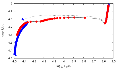
Figure 10: Evolution track of the TAMS 10+7 merger product (solid line) compared to the evolution track of a normal star of the same mass (dotted line). Points are plotted along the curves every $50\,000$ years. Note that the merger product spends a considerably longer time in the blue part of the region corresponding to the Hertzsprung gap than the normal star of the same mass.

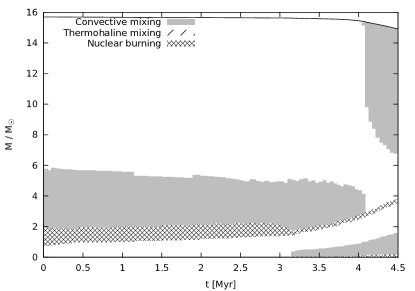
Figure 11: Kippenhahn diagram showing the evolution of the 10+7 ${\rm M}_{\odot}$TAMS merger product. Hydrogen burns in a shell around the helium core.

Figure 12: Core mass as functions of time for the TAMS 10+7 merger, in solar units. The dashed line represents the Schönberg-Chandrasekhar limit for the core mass. The merger product ignites helium after 3.1 Myr.

If the merger product has a hydrogen-depleted core (case P for TAMS or CHEX merger and some case M for TAMS or CHEX merger with $q\geq 0.99$) the evolution track can be very different from that of a normal star of the same mass or the merger products discussed in 4.3.1. These merger products do not have a core hydrogen-burning phase and begin their evolution with hydrogen shell burning on top of a helium core. After hydrogen exhaustion a normal star will quickly evolve through the Hertzsprung gap to the giant branch. Some of the merger products, however, have a long-lived phase of hydrogen shell burning in the blue part of the CMD and may even spend a significant part of their core helium burning lifetime while blue (Figures 10 and 13).

Figure 10 shows the evolution track of the TAMS 10+7 merger product. The location in the Hertzsprung-Russell diagram after the contraction phase is similar to that of a normal star of the same mass late on the main sequence but the evolution track lacks the distinctive hook that appears when the convective core disappears in a normal star. Helium ignition occurs in the Hertzsprung gap near $\log_{10}T_{\mathrm{eff}}=4.3$. The evolution of the interior is shown in Figure 11. The hydrogen burning shell is replenished by the thick convection zone above it. The extent of this convection zone is comparable to the extent of the convective core in a normal star of the same mass. As a result, the hydrogen burning shell mimics the hydrogen core of a normal star. Because of the presence of a convection zone above the burning shell the core mass grows slowly, increasing by only $0.5\,\mbox{${\rm M}_{\odot}$}$ in the first 3.1 Myr. After 3.1 Myr helium ignites in the centre. The convection zone that sustained the burning shell shrinks but does not disappear. This causes the core growth rate to increase after helium ignition.

An interesting aspect of this is that although the merger product is not a main sequence star, it would appear on the extension of the main sequence in a star cluster, and be counted as a blue straggler star. This is an exception to the result of Sills & Lombardi (1997) that mergers involving stars with hydrogen depleted cores do not produce blue stragglers.

The question of what allows a star to have an extended blue phase of hydrogen shell burning and what causes it to become a red giant instead has been debated extensively in the literature (Eggleton & Faulkner, 1981; Yahil & van den Horn, 1985; Applegate, 1988; Weiss, 1989; Eggleton & Cannon, 1991; Renzini et al., 1992; Sugimoto & Fujimoto, 2000; Stancliffe et al., 2009; Ball et al., 2012) and it is not clear that there is a single answer.

For hydrogen shell burning stars with an isothermal core the transition can be understood in terms of the maximum core mass, set by the virial theorem, for which the core can avoid contraction. While the core mass is below this limit the star remains in the blue part of the Hertzsprung-Russell diagram. This is the Schönberg-Chandrasekhar (SC) limit (Schönberg & Chandrasekhar, 1942; Kippenhahn & Weigert, 1990; Ball et al., 2012),

$$M_{\mathrm{SC}}=0.37\left(\frac{\mu_{\mathrm{env}}}{\mu_{\mathrm{c}}}\right)^{2}M.$$ (6)

Here $M$ is the total mass of the star, $\mu_{\mathrm{env}}$ the average mean molecular weight of the envelope and $\mu_{\mathrm{c}}$ the average mean molecular weight in the core. As long as the core mass is below the SC limit, the star can have an isothermal core and remain in thermal equilibrium. For normal stars in the mass range we consider here, the convective core on the main sequence is already more massive than this limit. However, this is not the case for the merger products.

In Figure 12 we show the core mass of the TAMS 10+7 merger product as a function of time. The dashed line shows the SC limit as calculated by Eq. (6). The core mass is below this limit until $3.1\,\mathrm{Myr}$. As the core mass approaches the SC limit the core contracts rapidly and heats up, leading to helium ignition. At this point the merger product is still in the blue part of the Hertzsprung-Russell diagram and becomes a blue supergiant, as can be seen from Figure 10. In Table 5 the merger products that form blue supergiants all have a helium core mass $M_{\mathrm{He}}$ smaller than the core mass $M_{\mathrm{He,ms}}$ of a normal star and $t_{\mathrm{HSB}}$ much smaller than $\tau_{\mathrm{HG}}$.

In addition to a prolonged blue phase of hydrogen shell burning some of our merger models also have a blue phase of helium core burning. The classical SC limit only applies to isothermal cores and is no longer relevant once a temperature gradient develops in the core and it cannot explain why some of these stars also stay blue during core helium burning. It is tempting to relate the occurrence of a blue phase of core helium burning to the occurrence of blue loops, which with our evolution code occur for stars below 12 $M_{\odot}$. The occurrence of blue loops has been linked to the efficiency of the hydrogen burning shell (Xu & Li, 2004) but as has been noted already by (Lauterborn et al., 1971), the presence of blue loops depends sensitively on the hydrogen profile in the envelope. Since the abundenace profile of our merger models can be very different from that of normal stars it is not surprising that the blue loops can be very different.

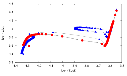
Figure 13: As Figure 10 for the TAMS 5+3.5 merger.

Not all stars with $M_{\mathrm{He}}<M_{\mathrm{He,ms}}$ form blue supergiants, however. The remnant of the TAMS 5+3.5 merger, shown in Figure 13, also stays in the blue part of the Hertzsprung-Russell diagram during a prolonged hydrogen shell burning phase, but in this case there is no blue phase of core helium burning. This is actually different from the main sequence reference model. In the reference model, helium ignition occurs near the tip of the giant branch ($L\approx 4.0L_{\odot}$) and the star then makes a blue loop before evolving up the AGB. The merger ignites helium in the Hertzsprung gap, before reaching the base of the giant branch, and continues to evolve up the giant branch until he exhaustion at $L\approx 4.2L_{\odot}$. It then evolves up the AGB.

4.3.3 An analytical recipe

An analytic recipe that can be used to predict merger product lifetimes and luminosities was developed by Glebbeek & Pols (2008) In brief, they found that the lifetime $t_{\mathrm{MS}}$ of the merger product can be found from $t_{\mathrm{MS}}=\tau_{\mathrm{MS}}(1-f_{\mathrm{app}}/\alpha)$, where

$$f_{\mathrm{app}}=\frac{1}{Q_{\mathrm{c}}(M)}\frac{1}{1-\phi}\frac{Q_{\mathrm{c},1}f_{1}+Q_{\mathrm{c},2}f_{2}q}{1+q}.$$ (7)

Here $\tau_{\mathrm{MS}}$ is the main sequence lifetime of a star of the same mass as the merger product, $f_{1}$ and $f_{2}$ are the ages of the primary and secondary star at the time of the merger, in units of their main sequence lifetimes, $\phi$ is the fraction of material lost in the collision, $Q_{\mathrm{c}}(M)$ is the fraction of hydrogen that is consumed during the main sequence by a star of mass $M$ (Glebbeek & Pols, 2008), $M$ is the total mass of the merger, $Q_{\mathrm{c},1}$ and $Q_{\mathrm{c},2}$ are the fractions of hydrogen consumed in the primary and secondary during their lifetime and $\alpha$ is a free parameter. Glebbeek & Pols (2008) found that a single value of $\alpha=1.67$ works well for mergers of low-mass stars. We find that $\alpha=1.14$ works well for the high-mass mergers discussed here (see Figure 14).

Some of our models have no main-sequence phase because they begin with hydrogen depleted cores. In Figure 14 these models fall along the bottom of the plot. Some of these have an extended blue phase of hydrogen shell burning, and we also plot these with the duration of the hydrogen shell burning phase in place of $t_{\mathrm{ms}}$. They then fall close to the predicted main-sequence lifetime.

Figure 14: Collision product lifetime compared to the prediction from Eq. (7). The models are indicated by $\circ$, the solid line is the prediction of Eq. (7) for $\alpha=1.14$. The dotted line is the lifetime according to the prescription of Hurley et al. (2000). Models with no main sequence but with an extended blue phase of hydrogen shell burning are plotted with $+\times$ for the duration of this phase.

4.4 Surface composition

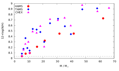
Figure 15: Surface abundance of nitrogen for our merger models, as a function of total mass. The dashed line represents our ZAMS composition.

Table 6: Surface abundances (by mass fraction) for the different merger products. The ZAMS line indicates the assumed ZAMS composition. The given abundance of CNO is multiplied by 1000.

stage	$M_{1}$	$M_{2}$	$X_{\mathrm{H}}$	$X_{\mathrm{He}}$	$X_{\mathrm{C}}$	$X_{\mathrm{N}}$	$X_{\mathrm{O}}$
	${\rm M}_{\odot}$	${\rm M}_{\odot}$			$\times 10^{3}$	$\times 10^{3}$	$\times 10^{3}$
ZAMS			0.700	0.280	3.52	1.04	10.04
HAMS	5	0.5	0.700	0.280	3.50	1.07	10.03
HAMS	10	1	0.699	0.281	3.43	1.22	9.95
HAMS	20	2	0.690	0.290	3.18	2.03	9.36
HAMS	40	4	0.683	0.297	3.04	2.71	8.77
HAMS	5	3.5	0.700	0.280	3.43	1.19	9.99
HAMS	10	7	0.698	0.282	3.27	1.59	9.74
HAMS	20	14	0.691	0.289	2.87	2.73	8.97
HAMS	40	28	0.662	0.318	2.39	4.97	7.06
TAMS	5	0.5	0.700	0.280	3.42	1.19	10.00
TAMS	10	1	0.697	0.283	3.37	1.35	9.88
TAMS	20	2	0.695	0.285	3.13	1.94	9.53
TAMS	40	4	0.682	0.298	3.05	2.64	8.85
TAMS	5	2	0.698	0.282	3.32	1.45	9.87
TAMS	10	4	0.689	0.291	2.60	3.31	8.70
TAMS	20	8	0.668	0.312	2.44	4.08	8.01
TAMS	40	16	0.625	0.355	1.85	6.85	5.63
TAMS	5	3.5	0.694	0.286	2.83	2.27	9.55
TAMS	10	7	0.691	0.289	2.53	3.23	8.86
TAMS	20	14	0.658	0.322	2.16	4.85	7.51
TAMS	40	28	0.615	0.365	1.81	7.03	5.50
TAMS	5	5	0.697	0.283	4.73	1.50	8.39
TAMS	10	10	0.687	0.293	3.11	2.90	8.59
TAMS	20	20	0.679	0.301	2.47	3.66	8.45
CHEX	5	0.5	0.700	0.280	3.66	1.09	9.86
CHEX	10	1	0.699	0.281	3.42	1.23	9.95
CHEX	20	2	0.696	0.284	3.31	1.59	9.69
CHEX	40	4	0.672	0.308	2.74	3.72	8.02
CHEX	5	2	0.697	0.283	3.32	1.40	9.90
CHEX	10	4	0.690	0.290	2.65	2.97	8.99
CHEX	20	8	0.665	0.315	2.16	4.83	7.53
CHEX	40	16	0.619	0.362	1.50	8.12	4.66
CHEX	5	3.5	0.696	0.284	3.13	1.78	9.72
CHEX	10	7	0.691	0.289	2.70	2.82	9.10
CHEX	20	14	0.665	0.315	2.24	4.61	7.67
CHEX	40	28	0.634	0.346	1.97	6.40	6.00
CHEX	5	5	0.694	0.286	4.51	1.94	8.19
CHEX	10	9.9	0.677	0.303	2.43	3.68	8.48
CHEX	20	19.8	0.649	0.331	2.17	4.98	7.37
CHEX	40	39.6	0.589	0.391	2.22	6.86	5.25
CHEX	5	5	0.694	0.286	4.51	1.94	8.19
CHEX	10	9.9	0.677	0.303	2.43	3.68	8.48
CHEX	20	19.8	0.649	0.331	2.17	4.98	7.37
CHEX	40	39.6	0.589	0.391	2.22	6.86	5.25

Although there is generally little or no mixing of hydrogen into the core of the merger product, the surface abundances can be strongly affected by material from the secondary star that is mixed into the envelope. In Table 6 we give the surface abundance (by mass fraction) for the main elements (H, He, C, N and O) and in Figure 15 we plot the surface nitrogen abundance as a function of total remnant mass. In both cases we list the abundances once the merger product has reached equilibrium and thermohaline convection has been allowed to modify the surface abundances.

Our lowest mass models show the least amount of mixing, in agreement with earlier findings in studies of mergers between low mass stars (Lombardi et al., 1996; Sills et al., 1997; Glebbeek et al., 2008). In contrast, our most massive merger products show much stronger mixing. The strongest enhancement is found for merger products resulting from more evolved parent stars.

It is clear from these results that substantial mixing can result from the merger process itself. In fact, the range of nitrogen enhancement is comparable for the range reported for B stars in the galactic field (Kilian, 1992; Nieva & Przybilla, 2012) and in the Magellanic Clouds (Hunter et al., 2007). It should be remembered, however, that the initial initial composition of our models is different from the derived compositions in these works and so our results are not directly comparable.

5 Summary & Conclusion

We have studied the evolution of stellar mergers formed by a collision involving massive stars. This is a first step in following the evolution of stellar merger runaways using detailed stellar models. Mass loss from the collisions is generally small, up to about 8% of the total mass for collisions involving equal mass stars at the end of the main sequence. The structure of these merger remnants can be well understood using a modification of the entropy sorting principle of Lombardi et al. (2002) presented by Gaburov et al. (2008b).

During the collision, the core of one of the parent stars can retain its identity and sink to the centre of the merger product. Whether this occurs for the core of the primary or the secondary depends on the buoyancy profile $A(m)$ in the parent stars. In cases with extreme mass ratio the secondary star as a whole can migrate to the centre of the merger product. In general we find that little hydrogen is mixed into the core of the merger product. However, the merger product can still have a hydrogen rich core if the core of the secondary displaces the core of the primary at the centre of the merger product. The shell with the location of highest temperature can initially be off-centre, resulting in a hydrogen-burning shell in the merger remnant. The burning front moves inward towards the centre on a thermal timescale. During the merger processed material can be mixed into the envelope of the merger product and produce strong nitrogen enhancement at the surface, especially for mergers involving evolved parent stars.

The main-sequence evolution of the merger remnant is qualitatively similar to the evolution of low mass collision products (Sills et al., 1997, 2001; Glebbeek et al., 2008; Glebbeek & Pols, 2008): in both cases helium enhancement of the lower envelope increases the star’s radius and luminosity. This increases the cross section of the merger remnant for a possible subsequent collision, which may be relevant when considering merger runaways. The main-sequence lifetime of massive merger products can be predicted in a similar manner to that of low mass merger products (Glebbeek & Pols, 2008).

Merger remnants that result from collisions with main-sequence stars at the end of the main sequence and where the core of the primary remains intact (case P) begin their evolution with an anomalously small hydrogen-depleted core and evolve differently from normal main-sequence stars or merger remnants that form with a hydrogen-rich core. The merger products can be in thermal equilibrium during hydrogen shell burning if the mass of the helium core is below the Schönberg-Chandrasekhar limit. In this case the star can appear as a blue straggler and ignite helium while still in the blue part of the Hertzsprung-Russell diagram. Observationally, many O and B stars appear to be in the Hertzsprung gap (Evans et al., 2006), between the end of the main sequence and the bluest part of the blue loop during core helium burning, although this conclusion is sensitive to the treatment of convective overshooting in the evolution tracks used for comparison. Stellar mergers involving turn-off stars, either through a collision as discussed in this work or by unstable case-B mass transfer in a binary, offer a mechanism to explain the presence of at least some stars in this part of the Hertzsprung-Russell diagram.

In this work we have manually coupled the stellar evolution calculations and the SPH calculations and performed a series of collision and subsequent evolution experiments. We coupled these codes by hand, because there was not yet an automated way to do this by the time we performed this research. The methods of converting stellar evolution code output to SPH realizations and vice versa, as described in this paper, have now been incorporated in the Astronomical Multipurpose Software Environment (AMUSE for short, see Portegies Zwart et al. 2009, 2013). AMUSE is a general-purpose framework for interconnecting scientific simulation programs using a homogeneous, unified software interface, and incorporates codes for stellar evolution, hydrodynamics, gravity and radiative transport. The entire software package including the scripts to perform the calculations in this paper can be downloaded for free from http://amusecode.org.

References

- Ahumada & Lapasset (1995) Ahumada, J. & Lapasset, E. 1995, AAPS, 109, 375
- Ahumada & Lapasset (2007) Ahumada, J. A. & Lapasset, E. 2007, A&A, 463, 789
- Angulo et al. (1999) Angulo, C., Arnould, M., Rayet, M., et al. 1999, Nuclear Physics A, 656, 3
- Antonini et al. (2011) Antonini, F., Lombardi, Jr., J. C., & Merritt, D. 2011, ApJ, 731, 128
- Applegate (1988) Applegate, J. H. 1988, ApJ, 329, 803
- Ball et al. (2012) Ball, W. H., Tout, C. A., & Żytkow, A. N. 2012, MNRAS, 421, 2713
- Bettwieser & Sugimoto (1984) Bettwieser, E. & Sugimoto, D. 1984, MNRAS, 208, 493
- Böhm-Vitense (1958) Böhm-Vitense, E. 1958, ZsAp, 46, 108
- Cassisi et al. (2007) Cassisi, S., Potekhin, A. Y., Pietrinferni, A., Catelan, M., & Salaris, M. 2007, ApJ, 661, 1094
- Charbonnel & Zahn (2007) Charbonnel, C. & Zahn, J.-P. 2007, A&A, 467, L15
- Chatterjee et al. (2013) Chatterjee, S., Rasio, F. A., Sills, A., & Glebbeek, E. 2013, ArXiv e-prints
- Clayton (1983) Clayton, D. D. 1983, Principles of stellar evolution and nucleosynthesis (Chicago: University of Chicago Press, 1983)
- Dale & Davies (2006) Dale, J. E. & Davies, M. B. 2006, MNRAS, 366, 1424
- Davies et al. (2004) Davies, M. B., Piotto, G., & de Angeli, F. 2004, MNRAS, 349, 129
- de Jager et al. (1988) de Jager, C., Nieuwenhuijzen, H., & van der Hucht, K. A. 1988, AAPS, 72, 259
- de Mink et al. (2013) de Mink, S. E., Langer, N., Izzard, R. G., Sana, H., & de Koter, A. 2013, ApJ, 764, 166
- Eggleton (1971) Eggleton, P. P. 1971, MNRAS, 151, 351
- Eggleton (1972) Eggleton, P. P. 1972, MNRAS, 156, 361
- Eggleton & Cannon (1991) Eggleton, P. P. & Cannon, R. C. 1991, ApJ, 383, 757
- Eggleton & Faulkner (1981) Eggleton, P. P. & Faulkner, J. 1981, in Astrophysics and Space Science Library, Vol. 88, Physical Processes in Red Giants, ed. I. Iben Jr. & A. Renzini, 179–182
- Evans et al. (2006) Evans, C. J., Lennon, D. J., Smartt, S. J., & Trundle, C. 2006, A&A, 456, 623
- Ferguson et al. (2005) Ferguson, J. W., Alexander, D. R., Allard, F., et al. 2005, ApJ, 623, 585
- Figer et al. (1998) Figer, D. F., Najarro, F., Morris, M., et al. 1998, ApJ, 506, 384
- Formicola et al. (2004) Formicola, A., Imbriani, G., Costantini, H., et al. 2004, Physics Letters B, 591, 61
- Freitag & Benz (2005) Freitag, M. & Benz, W. 2005, MNRAS, 358, 1133
- Gaburov et al. (2008a) Gaburov, E., Gualandris, A., & Portegies Zwart, S. 2008a, MNRAS, 384, 376
- Gaburov et al. (2008b) Gaburov, E., Lombardi, J. C., & Portegies Zwart, S. 2008b, MNRAS, 383, L5
- Glebbeek et al. (2009) Glebbeek, E., Gaburov, E., de Mink, S. E., Pols, O. R., & Portegies Zwart, S. F. 2009, A&A, 497, 255
- Glebbeek & Pols (2008) Glebbeek, E. & Pols, O. R. 2008, A&A, 488, 1017
- Glebbeek et al. (2008) Glebbeek, E., Pols, O. R., & Hurley, J. R. 2008, A&A, 488, 1007
- Glebbeek et al. (2010) Glebbeek, E., Sills, A., & Leigh, N. 2010, MNRAS, 408, 1267
- Herwig et al. (2006) Herwig, F., Austin, S. M., & Lattanzio, J. C. 2006, Phys. Rev. C, 73, 025802
- Hills & Day (1976) Hills, J. G. & Day, C. A. 1976, Astrophysical Letters, 17, 87
- Hunter et al. (2007) Hunter, I., Dufton, P. L., Smartt, S. J., et al. 2007, A&A, 466, 277
- Hurley et al. (2005) Hurley, J. R., Pols, O. R., Aarseth, S. J., & Tout, C. A. 2005, MNRAS, 363, 293
- Hurley et al. (2000) Hurley, J. R., Pols, O. R., & Tout, C. A. 2000, MNRAS, 315, 543
- Hurley et al. (2001) Hurley, J. R., Tout, C. A., Aarseth, S. J., & Pols, O. R. 2001, MNRAS, 323, 630
- Hut & Verbunt (1983) Hut, P. & Verbunt, F. 1983, Nature, 301, 587
- Iglesias & Rogers (1996) Iglesias, C. A. & Rogers, F. J. 1996, ApJ, 464, 943
- Johnson & Sandage (1955) Johnson, H. L. & Sandage, A. R. 1955, ApJ, 121, 616
- Kilian (1992) Kilian, J. 1992, A&A, 262, 171
- Kippenhahn et al. (1980) Kippenhahn, R., Ruschenplatt, G., & Thomas, H.-C. 1980, A&A, 91, 175
- Kippenhahn & Weigert (1990) Kippenhahn, R. & Weigert, A. 1990, Stellar Structure and Evolution (Stellar Structure and Evolution, XVI, 468 pp. 192 figs.. Springer-Verlag Berlin Heidelberg New York. Also Astronomy and Astrophysics Library)
- Lauterborn et al. (1971) Lauterborn, D., Refsdal, S., & Weigert, A. 1971, A&A, 10, 97
- Leigh et al. (2013) Leigh, N., Knigge, C., Sills, A., et al. 2013, MNRAS, 428, 897
- Leigh et al. (2007) Leigh, N., Sills, A., & Knigge, C. 2007, ApJ, 661, 210
- Leigh et al. (2011) Leigh, N., Sills, A., & Knigge, C. 2011, MNRAS, 415, 3771
- Lombardi et al. (2003) Lombardi, J. C., Thrall, A. P., Deneva, J. S., Fleming, S. W., & Grabowski, P. E. 2003, MNRAS, 345, 762
- Lombardi et al. (1996) Lombardi, Jr., J. C., Rasio, F. A., & Shapiro, S. L. 1996, ApJ, 468, 797
- Lombardi et al. (2002) Lombardi, Jr., J. C., Warren, J. S., Rasio, F. A., Sills, A., & Warren, A. R. 2002, ApJ, 568, 939
- Monaghan (2005) Monaghan, J. J. 2005, Reports on Progress in Physics, 68, 1703
- Nieva & Przybilla (2012) Nieva, M.-F. & Przybilla, N. 2012, A&A, 539, A143
- Piotto et al. (2004) Piotto, G., De Angeli, F., King, I. R., et al. 2004, ApJL, 604, L109
- Pols et al. (1995) Pols, O. R., Tout, C. A., Eggleton, P. P., & Han, Z. 1995, MNRAS, 274, 964
- Portegies Zwart et al. (2009) Portegies Zwart, S., McMillan, S., Harfst, S., et al. 2009, New A, 14, 369
- Portegies Zwart et al. (2013) Portegies Zwart, S., McMillan, S. L. W., van Elteren, E., Pelupessy, I., & de Vries, N. 2013, Computer Physics Communications, 183, 456
- Portegies Zwart et al. (2004) Portegies Zwart, S. F., Baumgardt, H., Hut, P., Makino, J., & McMillan, S. L. W. 2004, Nature, 428, 724
- Portegies Zwart et al. (1999) Portegies Zwart, S. F., Makino, J., McMillan, S. L. W., & Hut, P. 1999, A&A, 348, 117
- Renzini et al. (1992) Renzini, A., Greggio, L., Ritossa, C., & Ferrario, L. 1992, ApJ, 400, 280
- Rosswog (2009) Rosswog, S. 2009, New A Rev., 53, 78
- Sana et al. (2012) Sana, H., de Mink, S. E., de Koter, A., et al. 2012, Science, 337, 444
- Sandage (1953) Sandage, A. R. 1953, AJ, 58, 61
- Schönberg & Chandrasekhar (1942) Schönberg, M. & Chandrasekhar, S. 1942, ApJ, 96, 161
- Serenelli & Weiss (2005) Serenelli, A. & Weiss, A. 2005, A&A, 442, 1041
- Sills et al. (2005) Sills, A., Adams, T., & Davies, M. B. 2005, MNRAS, 358, 716
- Sills et al. (2002) Sills, A., Adams, T., Davies, M. B., & Bate, M. R. 2002, MNRAS, 332, 49
- Sills et al. (2001) Sills, A., Faber, J. A., Lombardi, Jr., J. C., Rasio, F. A., & Warren, A. R. 2001, ApJ, 548, 323
- Sills et al. (2013) Sills, A., Glebbeek, E., Chatterjee, S., & Rasio, F. A. 2013, ArXiv e-prints
- Sills & Lombardi (1997) Sills, A. & Lombardi, Jr., J. C. 1997, ApJL, 484, L51
- Sills et al. (1997) Sills, A., Lombardi, Jr., J. C., Bailyn, C. D., et al. 1997, ApJ, 487, 290
- Springel (2005) Springel, V. 2005, MNRAS, 364, 1105
- Stancliffe (2006) Stancliffe, R. J. 2006, MNRAS, 370, 1817
- Stancliffe et al. (2009) Stancliffe, R. J., Chieffi, A., Lattanzio, J. C., & Church, R. P. 2009, PASA, 26, 203
- Stancliffe et al. (2007) Stancliffe, R. J., Glebbeek, E., Izzard, R. G., & Pols, O. R. 2007, A&A, 464, L57
- Sugimoto & Fujimoto (2000) Sugimoto, D. & Fujimoto, M. Y. 2000, ApJ, 538, 837
- Suzuki et al. (2007) Suzuki, T. K., Nakasato, N., Baumgardt, H., et al. 2007, ApJ, 668, 435
- Vink et al. (2000) Vink, J. S., de Koter, A., & Lamers, H. J. G. L. M. 2000, A&A, 362, 295
- Vink et al. (2001) Vink, J. S., de Koter, A., & Lamers, H. J. G. L. M. 2001, A&A, 369, 574
- Weiss (1989) Weiss, A. 1989, A&A, 209, 135
- Xu & Li (2004) Xu, H. Y. & Li, Y. 2004, A&A, 418, 213
- Yahil & van den Horn (1985) Yahil, A. & van den Horn, L. 1985, ApJ, 296, 554