Power-Expected-Posterior Priors
for Variable Selection
in Gaussian Linear Models

Summary: In the context of the expected-posterior prior (EPP) approach to Bayesian variable selection in linear models, we combine ideas from power-prior and unit-information-prior methodologies to simultaneously (a) produce a minimally-informative prior and (b) diminish the effect of training samples. The result is that in practice our power-expected-posterior (PEP) methodology is sufficiently insensitive to the size $n^{*}$ of the training sample, due to PEP’s unit-information construction, that one may take $n^{*}$ equal to the full-data sample size $n$ and dispense with training samples altogether. This promotes stability of the resulting Bayes factors, removes the arbitrariness arising from individual training-sample selections, and greatly increases computational speed, allowing many more models to be compared within a fixed CPU budget. In this paper we focus on Gaussian linear models and develop our PEP methodology under two different baseline prior choices: the independence Jeffreys (or reference) prior, yielding the J-PEP posterior, and the Zellner $g$-prior, leading to Z-PEP. We find that, under the reference baseline prior, the asymptotics of PEP Bayes factors are equivalent to those of Schwartz’s BIC criterion, ensuring consistency of the PEP approach to model selection. We compare the performance of our method, in simulation studies and a real example involving prediction of air-pollutant concentrations from meteorological covariates, with that of a variety of previously-defined variants on Bayes factors (and other methods) for objective variable selection. Our PEP prior, due to its unit-information structure, leads to a variable-selection procedure that — in our empirical studies — (1) is systematically more parsimonious than the basic EPP with minimal training sample, while sacrificing no desirable performance characteristics to achieve this parsimony; (2) is robust to the size of the training sample, thus enjoying the advantages described above arising from the avoidance of training samples altogether; and (3) identifies maximum-a-posteriori models that achieve better out-of-sample predictive performance than that provided by standard EPPs, the $g$-prior, the hyper-$g$ prior, non-local priors, the LASSO and SCAD. Moreover, PEP priors are diffuse even when $n$ is not much larger than the number of covariates $p$, a setting in which EPPs can be far more informative than intended.

Keywords: Bayesian variable selection; Bayes factors; Consistency; Expected-posterior priors; Gaussian linear models; $g$-prior; Hyper-$g$ prior; LASSO; Non-local priors; Prior compatibility; Power-prior; Training samples; SCAD; Unit-information prior

Note: A glossary of abbreviations is given before the references at the end of the paper.

1 Introduction

A leading approach to Bayesian variable selection in regression models is based on posterior model probabilities and the corresponding posterior model odds, which are functions of Bayes factors. In the case of Gaussian regression models, on which we focus in this paper, an active area of research has emerged from attempts to use improper prior distributions in this approach; influential contributions include a variety of Bayes-factor variants (posterior, fractional and intrinsic: see, e.g., Aitkin (1991), O’Hagan (1995), and Berger and Pericchi (1996a, 1996b), respectively).

An important part of this work is focused on objective model selection methods (Casella and Moreno (2006); Moreno and Girón (2008); Casella et al. (2009)), having their source in the intrinsic priors originally introduced by Berger and Pericchi (1996b); these methods attempt to provide an approximate proper Bayesian interpretation for intrinsic Bayes factors (IBFs). Intrinsic priors can be considered as special cases of the expected-posterior prior (EPP) distributions of Pérez and Berger (2002), which have an appealing interpretation based on imaginary training data coming from prior predictive distributions. EPP distributions can accommodate improper baseline priors as a starting point, and the marginal likelihoods for all models are calculated up to the same normalizing constant; this overcomes the problem of indeterminacy of the Bayes factors. Moreover, as Consonni and Veronese (2008) note, “EPP is a method to make priors compatible across models, through their dependence on a common marginal data distribution; thus this methodology can be applied also with subjectively specified (proper) prior distributions.” However, in regression problems, the approach is based on one or more training samples chosen from the data, and this raises three new questions: how large should such training samples be, how should they be chosen, and how much do they influence the resulting posterior distributions?

In this paper we develop a minimally-informative prior and simultaneously diminish the effect of training samples on the EPP approach, by combining ideas from the power-prior method of Ibrahim and Chen (2000) and the unit-information-prior approach of Kass and Wasserman (1995): we raise the likelihood involved in the EPP distribution to the power $\frac{1}{n}$ (where $n$ denotes the sample size), to produce a prior information content equivalent to one data point. In this manner the effect of the imaginary/training sample is small with even modest $n$. Moreover, as will become clear in Section 5, in practice our power-expected-posterior (PEP) prior methodology, due to its low-information structure, is sufficiently insensitive to the size $n^{*}$ of the training sample that one may take $n^{*}=n$ and dispense with training samples altogether; this both removes the instability arising from the random choice of training samples and greatly reduces computation time.

As will be seen, PEP priors have an additional advantage over standard EPPs in settings, which arise with some frequency in disciplines such as bioinformatics/genomics (e.g., Council (2005)) and econometrics (e.g., Johnstone and Titterington (2009)), in which $n$ is not much larger than the number of covariates $p$: standard EPPs can be far more informative than intended in such situations, but the unit-information character of PEP priors ensures that this problem does not arise with the PEP approach.

PEP methodology can be implemented under any baseline prior choice, proper or improper. In this paper, results are presented for two different prior baseline choices: the Zellner $g$-prior and the independence Jeffreys prior. The conjugacy structure of the first of these choices (a) greatly increases calculation speed and (b) permits computation of the first two moments (see Section 1 of the web Appendix) of the resulting PEP prior, which offers flexibility in situations in which non-diffuse parametric prior information is available. When (on the other hand) little information, external to the present data set, about the parameters in the competing models is available, the PEP prior with the independence Jeffreys (or reference) baseline prior can be viewed as an objective model-selection technique, and the fact that the PEP posterior with the Jeffreys baseline is a special case of the posterior with the $g$-prior as baseline provides significant computational acceleration using the Jeffreys baseline.

With either choice of baseline prior, simple but efficient Monte-Carlo schemes for the estimation of the marginal likelihoods can be constructed in a straightforward manner. We find that the corresponding Bayes factors, under the reference baseline prior, are asymptotically equivalent to those of the BIC criterion (Schwarz, 1978); therefore the resulting PEP objective Bayesian variable-selection procedure is consistent.

We wish to emphasize two points, at the outset, regarding our intentions in developing PEP.

• The purpose of the paper is not to compare the performance of PEP priors with that of approaches such as mixtures of $g$-priors (e.g., Liang et al. (2008)) or BIC itself. The point here is to begin with EPPs, which are in wide use and which have the important property of compatibility across models (a feature that mixtures of $g$-priors lack), and to substantially improve EPPs by overcoming the difficulties that arise from their dependence on training samples.

• The paper focuses on a variable-selection problem in the class of linear models with fixed covariate space, where the number of available covariates is less than the sample size ($p<n$); we do not intend this method to be used in settings in which $p>n$.

The plan of the remainder of the paper is as follows. In the next two sub-Sections, to fix notation and ideas, we provide some preliminary details on the EPP approach, and we highlight difficulties that arise when implementing it in variable-selection problems. Our PEP prior methodology is described in detail in Section 2, and the resulting prior and posterior distributions are presented under the two different baseline prior choices mentioned above. In Section 3 we provide Monte-Carlo estimates of the marginal likelihood for our approach. Section 4 explores the limiting behavior of the resulting Bayes factors, under the reference baseline prior. In Section 5 we present illustrations of our method, under both baseline prior choices, in a simulation experiment and in a real-data example involving the prediction of atmospheric ozone levels from meteorological covariates; we also compare PEP with seven other variable-selection and coefficient-shrinkage methods on out-of-sample predictive performance. Finally, Section 6 concludes the paper with a brief summary and some ideas for further research.

1.1 Expected-posterior priors

Pérez and Berger (2002) developed priors for use in model comparison, through utilization of the device of “imaginary training samples” (Good (2004); Spiegelhalter and Smith (1988); Iwaki (1997)). They defined the expected-posterior prior (EPP) as the posterior distribution of a parameter vector for the model under consideration, averaged over all possible imaginary samples $\boldsymbol{y}^{*}$ coming from a “suitable” predictive distribution $m^{*}(\boldsymbol{y}^{*})$. Hence the EPP for the parameter vector $\boldsymbol{\theta}_{\ell}$ of any model $M_{\ell}\in\cal{M}$, with ${\cal M}$ denoting the model space, is

$$\pi^{E}_{\ell}(\boldsymbol{\theta}_{\ell})=\int\pi_{\ell}^{N}(\boldsymbol{\theta}_{\ell}|\boldsymbol{y}^{*})\,m^{*}(\boldsymbol{y}^{*})\,d\boldsymbol{y}^{*}\,,$$ (1)

where $\pi_{\ell}^{N}(\boldsymbol{\theta}_{\ell}|\boldsymbol{y}^{*})$ is the posterior $\boldsymbol{\theta}_{\ell}$ using a baseline prior $\pi_{\ell}^{N}(\boldsymbol{\theta}_{\ell})$ and data $\boldsymbol{y}^{*}$.

A question that naturally arises when using EPPs is which predictive distribution $m^{*}$ to employ for the imaginary data $\boldsymbol{y}^{*}$ in (1); Pérez and Berger (2002) discussed several choices for $m^{*}$. An attractive option, leading to the so-called base-model approach, arises from selecting a “reference” or “base” model $M_{0}$ for the training sample and defining $m^{*}(\boldsymbol{y}^{*})=m_{0}^{N}(\boldsymbol{y}^{*})\equiv f(\boldsymbol{y}^{*}|M_{0})$ to be the prior predictive distribution, evaluated at $\boldsymbol{y}^{*}$, for the reference model $M_{0}$ under the baseline prior $\pi_{0}^{N}(\boldsymbol{\theta}_{0})$. Then, for the reference model (i.e., when $M_{\ell}=M_{0}$), (1) reduces to $\pi^{E}_{0}(\boldsymbol{\theta}_{0})=\pi_{0}^{N}(\boldsymbol{\theta}_{0})$. Intuitively, the reference model should be at least as simple as the other competing models, and therefore a reasonable choice is to take $M_{0}$ to be a common sub-model of all $M_{\ell}\in{\cal M}$. This interpretation is close to the skeptical-prior approach described by Spiegelhalter et al. (2004, Section 5.5.2), in which a tendency toward the null hypothesis can be a-priori supported by centering the prior around values assumed by this hypothesis when no other information is available. In the variable-selection problem that we consider in this paper, the constant model (with no predictors) is clearly a good reference model that is nested in all the models under consideration. This selection makes calculations simpler, and additionally makes the EPP approach essentially equivalent to the arithmetic intrinsic Bayes factor approach of Berger and Pericchi (1996a).

One of the advantages of using EPPs is that impropriety of baseline priors causes no indeterminacy. There is no problem with the use of an improper baseline prior $\pi_{\ell}^{N}(\boldsymbol{\theta}_{\ell})$ in (1); the arbitrary constants cancel out in the calculation of any Bayes factor. Impropriety in $m^{*}$ also does not cause indeterminacy, because $m^{*}$ is common to the EPPs for all models. When a proper baseline prior is used, the EPP and the corresponding Bayes factors will be relatively insensitive to large values of the prior variances of the components of $\boldsymbol{\theta}_{\ell}$.

1.2 EPPs for variable selection in Gaussian linear models

In what follows, we examine variable-selection problems in Gaussian regression models. We consider two models $M_{\ell}$ (for $\ell=0,1$) with parameters $\boldsymbol{\theta}_{\ell}=(\boldsymbol{\beta}_{\ell}\,,\sigma_{\ell}^{2})$ and likelihood specified by

$$(\boldsymbol{Y}|\mathrm{X}_{\ell},\boldsymbol{\beta}_{\ell},\sigma_{\ell}^{2},M_{\ell})\sim N_{n}(\mathrm{X}_{\ell}\,\boldsymbol{\beta}_{\ell}\,,\sigma_{\ell}^{2}\,\mathrm{I}_{n})\,,$$ (2)

where $\boldsymbol{Y}=(Y_{1},\dots,Y_{n})$ is a vector containing the (real-valued) responses for all subjects, $\mathrm{X}_{\ell}$ is an $n\times d_{\ell}$ design matrix containing the values of the explanatory variables in its columns, $\mathrm{I}_{n}$ is the $n\times n$ identity matrix, $\boldsymbol{\beta}_{\ell}$ is a vector of length $d_{\ell}$ summarizing the effects of the covariates in model $M_{\ell}$ on the response $\boldsymbol{Y}$ and $\sigma_{\ell}^{2}$ is the error variance for model $M_{\ell}$. Variable selection based on EPP was originally presented by Pérez (1998); additional computational details have recently appeared in Fouskakis and Ntzoufras (2013a).

Suppose we have an imaginary/training data set $\boldsymbol{y}^{*}$, of size $n^{*}$, and design matrix $\mathrm{X}^{*}$ of size $n^{*}\times(p+1)\,$, where $p$ denotes the total number of available covariates. Then the EPP distribution, given by (1), will depend on $\mathrm{X}^{*}$ but not on $\boldsymbol{y}^{*}$, since the latter is integrated out. The selection of a minimal training sample has been proposed, to make the information content of the prior as small as possible, and this is an appealing idea. However, even the definition of minimal turns out to be open to question, since it is problem-specific (which models are we comparing?) and data-specific (how many variables are we considering?). One possibility is to specify the size of the minimal training sample either from (a) the dimension of the full model or (b) the dimension of the larger model in every pairwise model comparison performed. But, as will be seen below, when $n$ is not much larger than $p$, working with a minimal training sample can result in a prior that is far more influential than intended. Additionally, if the data derive from a highly structured situation, such as a randomized complete block experiment, most choices of a small part of the data to act as a training sample would be untypical.

Even if the minimal-training-sample idea is accepted, the problem of choosing such a subset of the full data set still remains. A natural solution involves computing the arithmetic mean (or some other summary of distributional center) of the Bayes factors over all possible training samples, but this approach can be computationally infeasible, especially when $n$ is much larger than $p$; for example, with $(n,p)=(100,50)$ and $(500,100)$ there are about $10^{29}$ and $10^{107}$ possible training samples, respectively, over which to average. An obvious choice at this point is to take a random sample from the set of all possible minimal training samples, but this adds an extraneous layer of Monte-Carlo noise to the model-comparison process. These difficulties have been well-documented in the literature, but the quest for a fully satisfactory solution is still on-going; for example, Berger and Pericchi (2004) note that they “were unable to define any type of ‘optimal’ training sample.”

An approach to choosing covariate values for the training sample has been proposed by researchers working with intrinsic priors (Casella and Moreno (2006); Girón et al. (2006); Moreno and Girón (2008); Casella et al. (2009)), since the same problem arises there too. They consider all pairwise model comparisons, either between the full model and each nested model, or between every model configuration and the null model, or between two nested models. They used training samples of size defined by the dimension of the full model in the first case, or by the dimension of the larger model in every pairwise comparison in the second and third cases. In all three settings, they proved that the intrinsic prior of the parameters of the larger model in each pairwise comparison, denoted here by $M_{k}$, depends on the imaginary covariate values only through the expression $\mathrm{W}_{k}^{-1}=(\mathrm{X}_{k}^{*^{T}}\mathrm{X}_{k}^{*})^{-1}$, where $\mathrm{X}_{k}^{*}$ is the imaginary design matrix of dimension $(d_{k}+1)\times d_{k}\,$ for a minimal training sample of size $(d_{k}+1)$. Then, driven by the idea of the arithmetic intrinsic Bayes factor, they avoid the dependence on the training sample by replacing $\mathrm{W}_{k}^{-1}$ with its average over all possible training samples of minimal size. This average can be proved to be equal to $\frac{n}{d_{k}+1}\left(\mathrm{X}_{k}^{T}\mathrm{X}_{k}\right)^{-1}$, where $\mathrm{X}_{k}$ is the design matrix of the larger model in each pairwise comparison, and therefore no subsampling from the $\mathrm{X}_{k}$ matrix is needed.

Although this approach seems intuitively sensible and dispenses with the extraction of the submatrices from $\mathrm{X}_{k}$, it is unclear if the procedure retains its intrinsic interpretation, i.e., whether it is equivalent to the arithmetic intrinsic Bayes factor. Furthermore, and more seriously, the resulting prior can be influential when $n$ is not much larger than $p$, in contrast to the prior we propose here, which has a unit-information interpretation.

2 Power-expected-posterior (PEP) priors

In this paper, starting with the EPP methodology, we combine ideas from the power-prior approach of Ibrahim and Chen (2000) and the unit-information-prior approach of Kass and Wasserman (1995). As a first step, the likelihoods involved in the EPP distribution are raised to the power $\frac{1}{\delta}$ and density-normalized. Then we set the power parameter $\delta$ equal to $n^{*}$, to represent information equal to one data point; in this way the prior corresponds to a sample of size one with the same sufficient statistics as the observed data. Regarding the size of the training sample, $n^{*}$, this could be any integer from $(p+2)$ (the minimal training sample size) to $n$. As will become clear below, we have found that significant advantages (and no disadvantages) arise from the choice $n^{*}=n$, from which $\mathrm{X}^{*}=\mathrm{X}$. In this way we completely avoid the selection of a training sample and its effects on the posterior model comparison, while still holding the prior information content at one data point. Sensitivity analysis for different choices of $n^{*}$ is performed as part of the first set of experimental results below (see Section 5.1).

For any $M_{\ell}\in{\cal M}$, we denote by $\pi_{\ell}^{N}(\boldsymbol{\beta}_{\ell},\sigma_{\ell}^{2}|\mathrm{X}_{\ell}^{*})$ the baseline prior for model parameters $\boldsymbol{\beta}_{\ell}$ and $\sigma_{\ell}^{2}$. Then the power-expected-posterior (PEP) prior $\pi_{\ell}^{PEP}(\boldsymbol{\beta}_{\ell},\sigma_{\ell}^{2}|\,\mathrm{X}_{\ell}^{*}\,,\delta)$ takes the following form:

$$\pi_{\ell}^{PEP}(\boldsymbol{\beta}_{\ell},\sigma_{\ell}^{2}\,|\,\mathrm{X}_{\ell}^{*}\,,\delta)=\int\pi_{\ell}^{N}(\boldsymbol{\beta}_{\ell},\sigma_{\ell}^{2}\,|\boldsymbol{y}^{*},\delta)\,m_{0}^{N}(\boldsymbol{y}^{*}|\,\mathrm{X}_{0}^{*}\,,\delta)\,d\boldsymbol{y}^{*}\,,$$ (3)

where

$$\pi_{\ell}^{N}(\boldsymbol{\beta}_{\ell},\sigma_{\ell}^{2}\,|\boldsymbol{y}^{*},\delta)=\frac{f(\boldsymbol{y}^{*}|\,\boldsymbol{\beta}_{\ell}\,,\sigma_{\ell}^{2},M_{\ell}\,;\mathrm{X}_{\ell}^{*}\,,\delta)\pi_{\ell}^{N}(\boldsymbol{\beta}_{\ell},\sigma_{\ell}^{2}|\mathrm{X}_{\ell}^{*})}{m_{\ell}^{N}(\boldsymbol{y}^{*}|\,\mathrm{X}_{\ell}^{*}\,,\delta)},$$ (4)

and $f(\boldsymbol{y}^{*}|\,\boldsymbol{\beta}_{\ell}\,,\sigma_{\ell}^{2},M_{\ell}\,;\mathrm{X}_{\ell}^{*}\,,\delta)\propto f(\boldsymbol{y}^{*}|\boldsymbol{\beta}_{\ell}\,,\sigma_{\ell}^{2},M_{\ell}\,;\mathrm{X}_{\ell}^{*})^{\frac{1}{\delta}}$ is the EPP likelihood raised to the power $\frac{1}{\delta}$ and density-normalized, i.e.,

$$f(\boldsymbol{y}^{*}|\,\boldsymbol{\beta}_{\ell}\,,\sigma_{\ell}^{2},M_{\ell}\,;\mathrm{X}_{\ell}^{*}\,,\delta) = \frac{f(\boldsymbol{y}^{*}|\boldsymbol{\beta}_{\ell},\sigma_{\ell}^{2},M_{\ell}\,;\mathrm{X}_{\ell}^{*})^{\frac{1}{\delta}}}{\int f(\boldsymbol{y}^{*}|\boldsymbol{\beta}_{\ell},\sigma_{\ell}^{2},M_{\ell}\,;\mathrm{X}_{\ell}^{*})^{\frac{1}{\delta}}d\boldsymbol{y}^{*}}=\frac{f_{N_{n^{*}}}(\boldsymbol{y}^{*}\,;\,\mathrm{X}_{\ell}^{*}\boldsymbol{\beta}_{\ell}\,,\sigma_{\ell}^{2}\,\mathrm{I}_{n^{*}})^{\frac{1}{\delta}}}{\int f_{N_{n^{*}}}(\boldsymbol{y}^{*}\,;\,\mathrm{X}_{\ell}^{*}\boldsymbol{\beta}_{\ell}\,,\sigma_{\ell}^{2}\,\mathrm{I}_{n^{*}})^{\frac{1}{\delta}}d\boldsymbol{y}^{*}}$$ (5)

$$= f_{N_{n^{*}}}(\boldsymbol{y}^{*}\,;\,\mathrm{X}_{\ell}^{*}\boldsymbol{\beta}_{\ell}\,,\delta\,\sigma_{\ell}^{2}\mathrm{I}_{n^{*}})\,;$$

here $f_{N_{d}}(\boldsymbol{y}\,;\,\boldsymbol{\mu},\boldsymbol{\Sigma})$ is the density of the $d$-dimensional Normal distribution with mean $\boldsymbol{\mu}$ and covariance matrix $\boldsymbol{\Sigma}$, evaluated at $\boldsymbol{y}$.

The distribution $m_{\ell}^{N}(\boldsymbol{y}^{*}|\,\mathrm{X}_{\ell}^{*}\,,\delta)$ appearing in (3) (for $\ell=0$) and (4) is the prior predictive distribution (or the marginal likelihood), evaluated at $\boldsymbol{y}^{*}$, of model $M_{\ell}$ with the power likelihood defined in (5) under the baseline prior $\pi^{N}_{\ell}(\boldsymbol{\beta}_{\ell},\sigma_{\ell}^{2}\,|\,\mathrm{X}_{\ell}^{*})$, i.e.,

$$m_{\ell}^{N}(\boldsymbol{y}^{*}|\,\mathrm{X}_{\ell}^{*}\,,\delta)=\int\!\!\int f_{N_{n^{*}}}(\boldsymbol{y}^{*}\,;\,\mathrm{X}_{\ell}^{*}\,\boldsymbol{\beta}_{\ell}\,,\delta\,\sigma_{\ell}^{2}\,\mathrm{I}_{n^{*}})\,\pi^{N}_{\ell}(\boldsymbol{\beta}_{\ell}\,,\sigma_{\ell}^{2}\,|\,\mathrm{X}_{\ell}^{*})\,d\boldsymbol{\beta}_{\ell}\,d\sigma_{\ell}^{2}\,.$$ (6)

From (3) and (4), the PEP prior can be re-written as

$$\pi_{\ell}^{PEP}(\boldsymbol{\beta}_{\ell},\sigma_{\ell}^{2}\,|\,\mathrm{X}_{\ell}^{*}\,,\delta)=\pi_{\ell}^{N}(\boldsymbol{\beta}_{\ell},\sigma_{\ell}^{2}|\mathrm{X}_{\ell}^{*})\int\frac{m_{0}^{N}(\boldsymbol{y}^{*}|\,\mathrm{X}_{0}^{*}\,,\delta)}{m_{\ell}^{N}(\boldsymbol{y}^{*}|\,\mathrm{X}_{\ell}^{*}\,,\delta)}\,f(\boldsymbol{y}^{*}|\,\boldsymbol{\beta}_{\ell}\,,\sigma_{\ell}^{2},M_{\ell}\,;\mathrm{X}_{\ell}^{*}\,,\delta)\,d\boldsymbol{y}^{*}\,.$$ (7)

Under the PEP prior distribution (7), the posterior distribution of the model parameters $(\boldsymbol{\beta}_{\ell}\,,\sigma_{\ell}^{2})$ is

$$\pi_{\ell}^{PEP}(\boldsymbol{\beta}_{\ell},\sigma_{\ell}^{2}|\boldsymbol{y};\mathrm{X}_{\ell},\mathrm{X}_{\ell}^{*},\delta) \propto \int\pi_{\ell}^{N}(\boldsymbol{\beta}_{\ell},\sigma_{\ell}^{2}|\boldsymbol{y},\boldsymbol{y}^{*};\mathrm{X}_{\ell},\mathrm{X}_{\ell}^{*},\delta)\times$$ (8)

$$\hskip 18.06749pt\,m_{\ell}^{N}(\boldsymbol{y}|\boldsymbol{y}^{*};\mathrm{X}_{\ell},\mathrm{X}_{\ell}^{*}\,,\delta)\,m_{0}^{N}(\boldsymbol{y}^{*}|\mathrm{X}_{0}^{*}\,,\delta)\,d\boldsymbol{y}^{*},$$

where $\pi_{\ell}^{N}(\boldsymbol{\beta}_{\ell},\sigma_{\ell}^{2}|\boldsymbol{y},\boldsymbol{y}^{*};\mathrm{X}_{\ell},\mathrm{X}_{\ell}^{*},\delta)$ and $m_{\ell}^{N}(\boldsymbol{y}|\boldsymbol{y}^{*};\mathrm{X}_{\ell},\mathrm{X}_{\ell}^{*}\,,\delta)$ are the posterior distribution of $(\boldsymbol{\beta}_{\ell},\sigma_{\ell}^{2})$ and the marginal likelihood of model $M_{\ell}$, respectively, using data $\boldsymbol{y}$ and design matrix $\mathrm{X}_{\ell}$ under prior $\pi_{\ell}^{N}(\boldsymbol{\beta}_{\ell}\,,\sigma_{\ell}^{2}|\boldsymbol{y}^{*};\,\mathrm{X}_{\ell}^{*}\,,\delta)$ — i.e., the posterior of $(\boldsymbol{\beta}_{\ell}\,,\sigma_{\ell}^{2})$ with power Normal likelihood (5) and baseline prior $\pi_{\ell}^{N}(\boldsymbol{\beta}_{\ell},\sigma_{\ell}^{2}|\mathrm{X}_{\ell}^{*})$.

In what follows we present results for the PEP prior using two specific baseline prior choices: the independence Jeffreys prior (improper) and the $g$-prior (proper). The first is the usual choice among researchers developing objective variable-selection methods, but the posterior results using this first baseline-prior choice can also be obtained as a limiting case of the results using the second baseline prior (see Section 2.3); usage of this second approach can lead to significant computational acceleration with the Jeffreys baseline prior.

2.1 PEP-prior methodology with the Jeffreys baseline prior: J-PEP

Here we use the independence Jeffreys prior (or reference prior) as the baseline prior distribution. Hence for $M_{\ell}\in{\cal M}$ we have

$$\pi_{\ell}^{N}(\boldsymbol{\beta}_{\ell}\,,\sigma^{2}\,|\,\mathrm{X}_{\ell}^{*})=\frac{c_{\ell}}{\sigma_{\ell}^{2}}\,,$$ (9)

where $c_{\ell}$ is an unknown normalizing constant; we refer to the resulting PEP prior as J-PEP.

2.1.1 Prior setup

Following (7) for the baseline prior (9) and the power likelihood specified in (5), the PEP prior, for any model $M_{\ell}\,$, now becomes

$$\pi_{\ell}^{\textit{J-PEP}}(\boldsymbol{\beta}_{\ell},\sigma_{\ell}^{2}|\mathrm{X}_{\ell}^{*}\,,\delta) = \int f_{N_{d_{\ell}}}\!\left[\boldsymbol{\beta}_{\ell}\,;\,\widehat{\boldsymbol{\beta}}_{\ell}^{*},\delta\,(\mathrm{X}_{\ell}^{*^{T}}\mathrm{X}_{\ell}^{*})^{-1}\sigma_{\ell}^{2}\right]\times$$ (10)

$$\hskip 18.06749ptf_{IG}\Big{(}\sigma_{\ell}^{2}\,;\,\frac{n^{*}-d_{\ell}}{2},\frac{RSS_{\ell}^{*}}{2\delta}\Big{)}\,m_{0}^{N}(\boldsymbol{y}^{*}|\mathrm{X}_{0}^{*}\,,\delta)\,d\boldsymbol{y}^{*}\,,$$

where $f_{IG}\left(y\,;\,a,b\right)$ is the density of the Inverse-Gamma distribution with parameters $a$ and $b$ and mean $\frac{b}{a-1}$, evaluated at $y$. Here $\widehat{\boldsymbol{\beta}}_{\ell}^{*}=(\mathrm{X}_{\ell}^{*^{T}}\mathrm{X}_{\ell}^{*})^{-1}\mathrm{X}_{\ell}^{*^{T}}\boldsymbol{y}^{*}$ is the MLE with outcome vector $\boldsymbol{y}^{*}$ and design matrix $\mathrm{X}_{\ell}^{*}$, and $RSS_{\ell}^{*}=\boldsymbol{y}{{}^{*}{{}^{T}}}\big{[}\mathrm{I}_{n^{*}}-\mathrm{X}_{\ell}^{*}(\mathrm{X}_{\ell}{{}^{*}{{}^{T}}}\mathrm{X}_{\ell}^{*})^{-1}\mathrm{X}_{\ell}{{}^{*}{{}^{T}}}\big{]}\boldsymbol{y}^{*}$ is the residual sum of squares using $(\boldsymbol{y}^{*},\mathrm{X}_{\ell}^{*})$ as data. The prior predictive distribution of any model $M_{\ell}$ with power likelihood defined in (5) under the baseline prior (9) is given by

$$m_{\ell}^{N}(\boldsymbol{y}^{*}\,|\,\mathrm{X}_{\ell}^{*}\,,\delta)=c_{\ell}\,\pi^{\frac{1}{2}(d_{\ell}-n^{*})}\,|\mathrm{X}_{\ell}^{*^{T}}\mathrm{X}_{\ell}^{*}|^{-\frac{1}{2}}\,\Gamma\left(\frac{n^{*}-d_{\ell}}{2}\right)RSS_{\ell}^{*^{-\left(\tfrac{n^{*}-d_{\ell}}{2}\right)}}\,.$$ (11)

2.1.2 Posterior distribution

For the PEP prior (10), the posterior distribution of the model parameters $(\boldsymbol{\beta}_{\ell}\,,\sigma_{\ell}^{2})$ is given by (8) with $f(\boldsymbol{\beta}_{\ell},\sigma_{\ell}^{2}|\boldsymbol{y},\boldsymbol{y}^{*},M_{\ell}\,;\mathrm{X}_{\ell},\mathrm{X}_{\ell}^{*},\delta)$ and $m_{\ell}^{N}(\boldsymbol{y}|\boldsymbol{y}^{*};\mathrm{X}_{\ell},\mathrm{X}_{\ell}^{*}\,,\delta)$ as the posterior distribution of $(\boldsymbol{\beta}_{\ell},\sigma_{\ell}^{2})$ and the marginal likelihood of model $M_{\ell}$, respectively, using data $\boldsymbol{y}$, design matrix $\mathrm{X}_{\ell}$, and the Normal-Inverse-Gamma distribution appearing in (10) as prior. Hence

$$\pi_{\ell}^{N}(\boldsymbol{\beta}_{\ell}|\sigma_{\ell}^{2},\boldsymbol{y},\boldsymbol{y}^{*};\mathrm{X}_{\ell},\mathrm{X}_{\ell}^{*},\delta) = f_{N_{d_{\ell}}}\big{(}\boldsymbol{\beta}_{\ell}\,;\,\widetilde{\boldsymbol{\beta}}^{N},\;\widetilde{\mathrm{\Sigma}}^{N}\sigma_{\ell}^{2}\big{)}\ \mbox{and}$$

$$\pi_{\ell}^{N}(\sigma_{\ell}^{2}|\boldsymbol{y},\boldsymbol{y}^{*};\mathrm{X}_{\ell},\mathrm{X}_{\ell}^{*},\delta) = f_{IG}(\sigma_{\ell}^{2}\,;\,\widetilde{a}_{\ell}^{N},\widetilde{b}_{\ell}^{N})\,,$$ (12)

with

$$\widetilde{\boldsymbol{\beta}}^{N} = \widetilde{\mathrm{\Sigma}}^{N}(\mathrm{X}_{\ell}^{T}\boldsymbol{y}+\delta^{-1}\mathrm{X}_{\ell}^{*^{T}}\boldsymbol{y}^{*}),\ \widetilde{\mathrm{\Sigma}}^{N}=\left[\mathrm{X}_{\ell}^{T}\mathrm{X}_{\ell}+\,\delta^{-1}\mathrm{X}_{\ell}^{*^{T}}\mathrm{X}_{\ell}^{*}\right]^{-1}\,\ \mbox{and}$$

$$\widetilde{a}_{\ell}^{N} = \frac{n+n^{*}-d_{\ell}}{2}\,,\ \widetilde{b}_{\ell}^{N}=\frac{SS_{\ell}^{N}+\delta^{-1}RSS_{\ell}^{*}}{2}\,.$$ (13)

Here

$$SS_{\ell}^{N} = \big{(}\boldsymbol{y}-\mathrm{X}_{\ell}\,\widehat{\boldsymbol{\beta}}_{\ell}^{*})^{T}\left[\mathrm{I}_{n}+\delta\,\mathrm{X}_{\ell}(\mathrm{X}_{\ell}^{*^{T}}\mathrm{X}_{\ell}^{*})^{-1}\mathrm{X}_{\ell}^{T}\right]^{-1}\big{(}\boldsymbol{y}-\mathrm{X}_{\ell}\,\widehat{\boldsymbol{\beta}}_{\ell}^{*})$$ (14)

and

$$m_{\ell}^{N}(\boldsymbol{y}|\boldsymbol{y}^{*};\mathrm{X}_{\ell},\mathrm{X}_{\ell}^{*}\,,\delta)=f_{St_{n}}\left\{\boldsymbol{y}\,;\,n^{*}-d_{\ell},\,\mathrm{X}_{\ell}\widehat{\boldsymbol{\beta}}_{\ell}^{*},\,\frac{RSS^{*}_{\ell}}{\delta(n^{*}-d_{\ell})}\left[\mathrm{I}_{n}+\delta\,\mathrm{X}_{\ell}(\mathrm{X}_{\ell}^{*^{T}}\mathrm{X}_{\ell}^{*})^{-1}\mathrm{X}_{\ell}^{T}\right]\right\}\,,$$ (15)

in which $St_{n}(\cdot\,;d,\boldsymbol{\mu},\Sigma)$ is the multivariate Student distribution in $n$ dimensions with $d$ degrees of freedom, location $\boldsymbol{\mu}$ and scale $\Sigma$. Thus the posterior distribution of the model parameters $(\boldsymbol{\beta}_{\ell}\,,\sigma_{\ell}^{2})$ under the PEP prior (10) is

$$\pi_{\ell}^{\textit{J-PEP}}(\boldsymbol{\beta}_{\ell},\sigma_{\ell}^{2}|\boldsymbol{y};\mathrm{X}_{\ell},\mathrm{X}_{\ell}^{*},\delta) \propto \int f_{N_{d_{\ell}}}\big{(}\boldsymbol{\beta}_{\ell}\,;\,\widetilde{\boldsymbol{\beta}}^{N},\;\widetilde{\mathrm{\Sigma}}^{N}\sigma_{\ell}^{2}\big{)}\,f_{IG}(\sigma_{\ell}^{2}\,;\,\widetilde{a}_{\ell}^{N},\widetilde{b}_{\ell}^{N})\times$$ (16)

$$\hskip 18.06749ptm_{\ell}^{N}(\boldsymbol{y}|\boldsymbol{y}^{*};\,\mathrm{X}_{\ell},\mathrm{X}_{\ell}^{*}\,,\delta)\,m_{0}^{N}(\boldsymbol{y}^{*}|\mathrm{X}_{0}^{*}\,,\delta)\,d\boldsymbol{y}^{*}\,,$$

with $m_{0}^{N}(\boldsymbol{y}^{*}|\mathrm{X}_{0}^{*}\,,\delta)$ given in (11). A detailed MCMC scheme for sampling from this distribution is presented in Section 2 of the web Appendix.

2.2 PEP-prior methodology with the $g$-prior as baseline: Z-PEP

Here we use the Zellner $g$-prior as the baseline prior distribution; in other words, for any $M_{\ell}\in{\cal M}$

$$\pi_{\ell}^{N}(\boldsymbol{\beta}_{\ell}|\sigma_{\ell}^{2}\,;\,\mathrm{X}_{\ell}^{*})=f_{N_{d_{\ell}}}\left[\boldsymbol{\beta}_{\ell}\,;\,\boldsymbol{0},g\,(\mathrm{X}_{\ell}^{*^{T}}\mathrm{X}_{\ell}^{*})^{-1}\sigma_{\ell}^{2}\right]\textrm{ and }\pi_{\ell}^{N}(\sigma_{\ell}^{2})=f_{IG}\left(\sigma_{\ell}^{2}\,;\,a_{\ell},b_{\ell}\right)\,.$$ (17)

We refer to the resulting PEP prior as Z-PEP. Note that the usual improper reference prior for $\sigma_{\ell}$ could easily be used instead, but for computational reasons we prefer here to use the Inverse-Gamma prior (recall that for $a_{\ell}$ and $b_{\ell}$ approximately equal to zero, the Inverse-Gamma prior degenerates to the improper reference prior).

2.2.1 Prior setup

For any model $M_{\ell}$, under the baseline prior setup (17) and the power likelihood (5), the prior predictive distribution is

$$m_{\ell}^{N}(\boldsymbol{y}^{*}\,|\,\mathrm{X}_{\ell}^{*}\,,\delta)=f_{St_{n^{*}}}\Big{(}\boldsymbol{y}^{*}\,;2\,a_{\ell},\boldsymbol{0},\frac{b_{\ell}}{a_{\ell}}{\Lambda_{\ell}^{*}}^{-1}\Big{)}\,,$$ (18)

where

$${\Lambda_{\ell}^{*}}^{-1}=\delta\left[\mathrm{I}_{n^{*}}-\frac{g}{g+\delta}\mathrm{X}_{\ell}^{*}\left({\mathrm{X}_{\ell}^{*}}^{T}\mathrm{X}_{\ell}^{*}\right)^{-1}{\mathrm{X}_{\ell}^{*}}^{T}\right]^{-1}=\delta\,\mathrm{I}_{n^{*}}+g\,\mathrm{X}_{\ell}^{*}\left({\mathrm{X}_{\ell}^{*}}^{T}\mathrm{X}_{\ell}^{*}\right)^{-1}{\mathrm{X}_{\ell}^{*}}^{T}\,.$$ (19)

In the special case of the constant model, (19) simplifies to $\left(\delta\,\mathrm{I}_{n^{*}}+\frac{g}{n}\boldsymbol{1}_{n^{*}}\boldsymbol{1}_{n^{*}}^{T}\right)$, where $\boldsymbol{1}_{n^{*}}$ is a vector of length $n^{*}$ with all elements equal to one.

Following (7) for the baseline prior (17) and the power likelihood specified in (5), the Z-PEP prior, for any model $M_{\ell}\,$, now becomes

$$\pi_{\ell}^{\textit{Z-PEP}}(\boldsymbol{\beta}_{\ell},\sigma_{\ell}^{2}|\mathrm{X}_{\ell}^{*}\,,\delta) = \int f_{N_{d_{\ell}}}\left[\boldsymbol{\beta}_{\ell}\,;\,w\,\widehat{\boldsymbol{\beta}}_{\ell}^{*},w\,\delta\,(\mathrm{X}_{\ell}^{*^{T}}\mathrm{X}_{\ell}^{*})^{-1}\sigma_{\ell}^{2}\right]\times$$ (20)

$$\hskip 18.06749ptf_{IG}\Big{(}\sigma_{\ell}^{2}\,;\,a_{\ell}+\frac{n^{*}}{2},b_{\ell}+\frac{SS_{\ell}^{*}}{2}\Big{)}\,m_{0}^{N}(\boldsymbol{y}^{*}|\mathrm{X}_{0}^{*}\,,\delta)\,d\boldsymbol{y}^{*}\,.$$

Here $w=\frac{g}{g+\delta}$ is the shrinkage weight, $\widehat{\boldsymbol{\beta}}_{\ell}^{*}=(\mathrm{X}_{\ell}^{*^{T}}\mathrm{X}_{\ell}^{*})^{-1}\mathrm{X}_{\ell}^{*^{T}}\boldsymbol{y}^{*}$ is the MLE with outcome vector $\boldsymbol{y}^{*}$ and design matrix $\mathrm{X}_{\ell}^{*}$, and $SS_{\ell}^{*}=\boldsymbol{y}^{*^{T}}\Lambda_{\ell}^{*}\,\boldsymbol{y}^{*}$ is the posterior sum of squares.

The prior mean vector and covariance matrix of $\boldsymbol{\beta}_{\ell}$, and the prior mean and variance of $\sigma_{\ell}^{2}$, can be calculated analytically from these expressions; details are available in Theorems 1 and 2 in Section 1 of the web Appendix.

2.2.2 Posterior distribution

The distributions $\pi_{\ell}^{N}(\boldsymbol{\beta}_{\ell},\sigma_{\ell}^{2}|\boldsymbol{y},\boldsymbol{y}^{*};\mathrm{X}_{\ell},\mathrm{X}_{\ell}^{*},\delta)$ and $m_{\ell}^{N}(\boldsymbol{y}|\boldsymbol{y}^{*};\mathrm{X}_{\ell},\mathrm{X}_{\ell}^{*}\,,\delta)$ involved in the calculation of the posterior distribution (8) are now the posterior distribution of $(\boldsymbol{\beta}_{\ell},\sigma_{\ell}^{2})$ and the marginal likelihood of model $M_{\ell}$, respectively, using data $\boldsymbol{y}$, design matrix $\mathrm{X}_{\ell}$, and $\pi_{\ell}^{N}(\boldsymbol{\beta}_{\ell}\,,\sigma_{\ell}^{2}|\boldsymbol{y}^{*};\,\mathrm{X}_{\ell}^{*}\,,\delta)$ as a prior density (which is the Normal-Inverse-Gamma distribution appearing in (20)). Therefore the posterior distribution of the model parameters $(\boldsymbol{\beta}_{\ell}\,,\sigma_{\ell}^{2})$ under the Z-PEP prior (20) is given by

$$\pi_{\ell}^{\textit{Z-PEP}}(\boldsymbol{\beta}_{\ell},\sigma_{\ell}^{2}|\boldsymbol{y};\mathrm{X}_{\ell},\mathrm{X}_{\ell}^{*},\delta) \propto \int f_{N_{d_{\ell}}}\big{(}\boldsymbol{\beta}_{\ell}\,;\,\widetilde{\boldsymbol{\beta}}^{N},\;\widetilde{\mathrm{\Sigma}}^{N}\sigma_{\ell}^{2}\big{)}\,f_{IG}(\sigma_{\ell}^{2}\,;\,\widetilde{a}_{\ell}^{N},\widetilde{b}_{\ell}^{N})\times$$ (21)

$$\hskip 18.06749ptm_{\ell}^{N}(\boldsymbol{y}|\boldsymbol{y}^{*};\,\mathrm{X}_{\ell},\mathrm{X}_{\ell}^{*}\,,\delta)\,m_{0}^{N}(\boldsymbol{y}^{*}|\mathrm{X}_{0}^{*}\,,\delta)\,d\boldsymbol{y}^{*}\,,$$

with

$$\widetilde{\boldsymbol{\beta}}^{N} = \widetilde{\mathrm{\Sigma}}^{N}(\mathrm{X}_{\ell}^{T}\boldsymbol{y}+\delta^{-1}\mathrm{X}_{\ell}^{*^{T}}\boldsymbol{y}^{*}),\ \widetilde{\mathrm{\Sigma}}^{N}=\left[\mathrm{X}_{\ell}^{T}\mathrm{X}_{\ell}+(w\,\delta)^{-1}\mathrm{X}_{\ell}^{*^{T}}\mathrm{X}_{\ell}^{*}\right]^{-1}\,\ \textrm{and}$$

$$\widetilde{a}_{\ell}^{N} = \frac{n+n^{*}}{2}+a_{\ell}\,,\ \widetilde{b}_{\ell}^{N}=\frac{SS_{\ell}^{N}+SS_{\ell}^{*}}{2}+b_{\ell}\,.$$ (22)

Here

$$SS_{\ell}^{N}=\big{(}\boldsymbol{y}-w\,\mathrm{X}_{\ell}\,\widehat{\boldsymbol{\beta}}_{\ell}^{*})^{T}\left[\mathrm{I}_{n}+\delta\,w\,\mathrm{X}_{\ell}(\mathrm{X}_{\ell}^{*^{T}}\mathrm{X}_{\ell}^{*})^{-1}\mathrm{X}_{\ell}^{T}\right]^{-1}\big{(}\boldsymbol{y}-w\,\mathrm{X}_{\ell}\,\widehat{\boldsymbol{\beta}}_{\ell}^{*})\,,$$ (23)

while

$$m_{\ell}^{N}(\boldsymbol{y}|\boldsymbol{y}^{*};\mathrm{X}_{\ell},\mathrm{X}_{\ell}^{*}\,,\delta)=f_{St_{n}}\left\{\boldsymbol{y}\,;\,2\,a_{\ell}+n^{*},w\,\mathrm{X}_{\ell}\widehat{\boldsymbol{\beta}}_{\ell}^{*},\,\frac{2b_{\ell}+SS^{*}_{\ell}}{2\,a_{\ell}+n^{*}}\left[\mathrm{I}_{n}+w\,\delta\,\mathrm{X}_{\ell}(\mathrm{X}_{\ell}^{*^{T}}\mathrm{X}_{\ell}^{*})^{-1}\mathrm{X}_{\ell}^{T}\right]\right\}\,,$$ (24)

and $m_{0}^{N}(\boldsymbol{y}^{*}|\mathrm{X}_{0}^{*}\,,\delta)$ is given in (18). A detailed MCMC scheme for sampling from this distribution is presented in Section 2 of the web Appendix.

2.2.3 Specification of hyper-parameters

The marginal likelihood for the Z-PEP prior methodology, using the $g$-prior as a baseline, depends on the selection of the hyper-parameters $g$, $a_{\ell}$ and $b_{\ell}$. We make the following proposals for specifying these quantities, in settings in which strong prior information about the parameter vectors in the models is not available.

The parameter $g$ in the Normal baseline prior is set to $\delta\,n^{*}$, so that with $\delta=n^{*}$ we use $g=(n^{*})^{2}$. This choice will make the $g$-prior contribute information equal to one data point within the posterior $\pi_{\ell}^{N}(\boldsymbol{\beta}_{\ell}\,,\sigma_{\ell}^{2}|\boldsymbol{y}^{*};\,\mathrm{X}_{\ell}^{*}\,,\delta)$. In this manner, the entire Z-PEP prior contributes information equal to $\left(1+\frac{1}{\delta}\right)$ data points.

We set the parameters $a_{\ell}$ and $b_{\ell}$ in the Inverse-Gamma baseline prior to 0.01, yielding a baseline prior mean of 1 and variance of 100 (i.e., a large amount of prior uncertainty) for the precision parameter; our method yields similar results across a broad range of small values of $a_{\ell}$ and $b_{\ell}$. (If strong prior information about the model parameters is available, Theorems 1 and 2 in Section 1 of the web Appendix can be used to guide the choice of $a_{\ell}$ and $b_{\ell}$.)

2.3 Connection between the J-PEP and Z-PEP distributions

By comparing the posterior distributions under the two different baseline schemes described in Sections 2.1 and 2.2, it is straightforward to prove that they coincide under the following conditions $(*)$: large $g$ (and therefore $w\approx 1$), $a_{\ell}=-\frac{d_{\ell}}{2}$ and $b_{\ell}=0$.

To be more specific, the posterior distribution in both cases takes the form of equation (16). The parameters of the Normal-Inverse-Gamma distribution (see equations (2.2.2)) involved in the posterior distribution using the $g$-prior as baseline become equal to the corresponding parameters for the Jeffreys baseline (see equations (2.1.2)) with parameter values $(*)$. Similarly, the conditional marginal likelihood $m_{\ell}^{N}(\boldsymbol{y}|\boldsymbol{y}^{*};\,\mathrm{X}_{\ell},\mathrm{X}_{\ell}^{*}\,,\delta)$ under the two baseline priors (see equations (15) and (24)) becomes the same under conditions $(*)$.

Finally, the prior predictive densities $m_{0}^{N}(\boldsymbol{y}^{*}|\mathrm{X}_{0}^{*}\,,\delta)$ involved in equations (16) and (21) can be written as $m_{0}^{N}(\boldsymbol{y}^{*}|\mathrm{X}_{0}^{*}\,,\delta)\propto(2\,b_{\ell}\,+\,SS_{\ell}^{*})^{-\frac{n^{*}+a_{\ell}}{2}}$ for the $g$-prior baseline and as $m_{0}^{N}(\boldsymbol{y}^{*}|\mathrm{X}_{0}^{*}\,,\delta)\propto RSS_{\ell}^{*^{-\frac{n^{*}-d_{\ell}}{2}}}$ for the Jeffreys baseline. For large values of $g$, $SS_{\ell}^{*}\rightarrow\delta^{-1}RSS_{\ell}^{*}$, and the two un-normalized prior predictive densities clearly become equal if we further set $a_{\ell}=-\frac{d_{\ell}}{2}$ and $b_{\ell}=0$. Any differences in the normalizing constants of $m_{0}^{N}(\boldsymbol{y}^{*}|\mathrm{X}_{0}^{*}\,,\delta)$ cancel out when normalizing the posterior distributions (16) and (21).

For these reasons, the posterior results using the Jeffreys prior as baseline can be obtained as a special (limiting) case of the results using the $g$-prior as baseline. This can be beneficial for the computation of the posterior distribution, which is detailed in Section 2 of the web Appendix, and for the estimation of the marginal likelihood presented in Section 3.

3 Marginal-likelihood computation

Under the PEP-prior approach, it is straightforward to show that the marginal likelihood of any model $M_{\ell}\in{\cal M}$ is

$$m^{PEP}_{\ell}(\boldsymbol{y}|\mathrm{X}_{\ell}\,,\mathrm{X}_{\ell}^{*}\,,\delta)=m_{\ell}^{N}(\boldsymbol{y}|\mathrm{X}_{\ell}\,,\mathrm{X}_{\ell}^{*}\,)\int\frac{m_{\ell}^{N}(\boldsymbol{y}^{*}|\boldsymbol{y},\mathrm{X}_{\ell},\mathrm{X}_{\ell}^{*}\,,\delta)}{m_{\ell}^{N}(\boldsymbol{y}^{*}|\mathrm{X}_{\ell}^{*}\,,\delta)}\,m_{0}^{N}(\boldsymbol{y}^{*}|\mathrm{X}_{0}^{*}\,,\delta)\,d\boldsymbol{y}^{*}\,.$$ (25)

Note that in the above expression $m_{\ell}^{N}(\boldsymbol{y}|\mathrm{X}_{\ell}\,,\mathrm{X}_{\ell}^{*})$ is the marginal likelihood of model $M_{\ell}$ for the actual data under the baseline prior and therefore, under the baseline $g$-prior (17), is given by

$$m_{\ell}^{N}(\boldsymbol{y}|\mathrm{X}_{\ell}\,,\mathrm{X}_{\ell}^{*})=f_{St_{n}}\left\{\boldsymbol{y}\,;2\,a_{\ell},\boldsymbol{0},\frac{b_{\ell}}{a_{\ell}}\left[\mathrm{I}_{n}+g\,\mathrm{X}_{\ell}\left(\mathrm{X}_{\ell}^{*^{T}}\mathrm{X}_{\ell}^{*}\right)^{-1}{\mathrm{X}_{\ell}}^{T}\right]\right\}\,;$$ (26)

under the Jeffreys baseline prior (9), $m_{\ell}^{N}(\boldsymbol{y}|\mathrm{X}_{\ell}\,,\mathrm{X}_{\ell}^{*})$ is given by equation (11) with data $(\boldsymbol{y},\mathrm{X}_{\ell})$.

In settings in which the marginal likelihood (25) is not analytically tractable, we have obtained four possible Monte-Carlo estimates. In Section 5.1.1 we show that two of these possibilities are far less accurate than the other two; we detail the less successful approaches in Section 3 of the web Appendix. The other two (more accurate) methods are as follows:

1. Generate $\boldsymbol{y}^{*(t)}\,(t=1,\dots,T)$ from $m_{\ell}^{N}(\boldsymbol{y}^{*}|\boldsymbol{y},\,\mathrm{X}_{\ell},\mathrm{X}_{\ell}^{*}\,,\delta)$ and estimate the marginal likelihood by

   $$\hat{m}^{PEP}_{\ell}(\boldsymbol{y}|\mathrm{X}_{\ell}\,,\mathrm{X}_{\ell}^{*}\,,\delta)=m_{\ell}^{N}(\boldsymbol{y}|\mathrm{X}_{\ell},\mathrm{X}_{\ell}^{*})\left[\frac{1}{T}\sum_{t=1}^{T}\frac{m_{0}^{N}(\boldsymbol{y}^{*(t)}|\mathrm{X}_{0}^{*}\,,\delta)}{m_{\ell}^{N}(\boldsymbol{y}^{*(t)}|\mathrm{X}_{\ell}^{*}\,,\delta)}\right]\,.$$ (27)

2. Generate $\boldsymbol{y}^{*(t)}\,(t=1,\dots,T)$ from $m_{\ell}^{N}(\boldsymbol{y}^{*}|\,\boldsymbol{y};\mathrm{X}_{\ell}\,,\mathrm{X}_{\ell}^{*}\,,\delta)$ and estimate the marginal likelihood by

   $$\hat{m}^{PEP}_{\ell}(\boldsymbol{y}|\mathrm{X}_{\ell}\,,\mathrm{X}_{\ell}^{*}\,,\delta)=m_{0}^{N}(\boldsymbol{y}|\mathrm{X}_{0},\mathrm{X}_{0}^{*})\left[\frac{1}{T}\sum_{t=1}^{T}\frac{m_{\ell}^{N}(\boldsymbol{y}|\,\boldsymbol{y}^{*(t)};\mathrm{X}_{\ell},\mathrm{X}_{\ell}^{*}\,,\delta)}{m_{0}^{N}(\boldsymbol{y}|\,\boldsymbol{y}^{*(t)};\mathrm{X}_{0},\mathrm{X}_{0}^{*}\,,\delta)}\frac{m_{0}^{N}(\boldsymbol{y}^{*(t)}|\,\boldsymbol{y};\mathrm{X}_{0},\mathrm{X}_{0}^{*}\,,\delta)}{m_{\ell}^{N}(\boldsymbol{y}^{*(t)}|\,\boldsymbol{y};\mathrm{X}_{\ell},\mathrm{X}_{\ell}^{*}\,,\delta)}\right]\,.$$ (28)

Monte-Carlo schemes (1) and (2) generate imaginary data from the posterior predictive distribution of the model under consideration, and thus we expect them to be relatively accurate. Moreover, in the second Monte-Carlo scheme, when we estimate Bayes factors we only need to evaluate posterior predictive distributions, which are available even in the case of improper baseline priors. Closed-form expressions for the posterior predictive distributions can be found in Section 2 of the web Appendix.

Using arguments similar to those in Section 2.3, it is clear that the marginal likelihoods $m^{PEP}_{\ell}(\boldsymbol{y}|\mathrm{X}_{\ell}\,,\mathrm{X}_{\ell}^{*}\,,\delta)$ under the two baseline prior choices considered in this paper will yield the same posterior odds and model probabilities for $g\rightarrow\infty$, $a_{\ell}=-\frac{d_{\ell}}{2}$ and $b_{\ell}=0$. This is because the posterior predictive densities involved in the expressions for $m^{PEP}_{\ell}(\boldsymbol{y}|\mathrm{X}_{\ell}\,,\mathrm{X}_{\ell}^{*}\,,\delta)$ become the same for the above-mentioned prior parameter values, while the corresponding prior predictive density will be the same up to normalizing constants (common to all models) that cancel out in the calculation.

4 Consistency of the J-PEP Bayes factor

Here we present a condensed version of a proof that Bayes factors based on the J-PEP approach are consistent for model selection; additional details are available in Fouskakis and Ntzoufras (2013b).

The PEP prior (7) can be rewritten as

$$\pi_{\ell}^{PEP}(\boldsymbol{\beta}_{\ell},\sigma_{\ell}^{2}|\mathrm{X}_{\ell}^{*},\delta) = \int\!\!\int\pi_{\ell}^{PEP}(\boldsymbol{\beta}_{\ell},\sigma_{\ell}^{2}|\boldsymbol{\beta}_{0},\sigma_{0}^{2};\mathrm{X}_{\ell}^{*},\delta)\,\pi_{0}^{N}(\boldsymbol{\beta}_{0},\sigma_{0}^{2}|{\mathrm{X}}_{0}^{*})\,d\boldsymbol{\beta}_{0}\,d\sigma_{0}^{2}\,,$$ (29)

in which the conditional PEP prior is given by

$$\pi_{\ell}^{PEP}(\boldsymbol{\beta}_{\ell},\sigma_{\ell}^{2}|\boldsymbol{\beta}_{0},\sigma_{0}^{2};\mathrm{X}_{\ell}^{*},\delta)=\int\frac{f(\boldsymbol{y}^{*}|\boldsymbol{\beta}_{\ell},\sigma_{\ell}^{2},M_{\ell};\mathrm{X}_{\ell}^{*},\delta)\,f(\boldsymbol{y}^{*}|\boldsymbol{\beta}_{0},\sigma_{0}^{2},M_{0};\mathrm{X}_{0}^{*},\delta)\,\pi^{N}(\boldsymbol{\beta}_{\ell},\sigma_{\ell}^{2}|\mathrm{X}_{\ell}^{*})}{m_{\ell}^{N}(\boldsymbol{y}^{*}|\mathrm{X}_{\ell}^{*},\delta)}\,d\boldsymbol{y}^{*}\,.$$ (30)

For the J-PEP prior, resulting from the baseline prior (9), it can be shown — following a line of reasoning similar to that in Moreno et al. (2003) — that

$$\pi_{\ell}^{\textit{J-PEP}}(\boldsymbol{\beta}_{\ell},\sigma_{\ell}^{2}|\boldsymbol{\beta}_{0},\sigma_{0}^{2};\mathrm{X}_{\ell}^{*},\delta) = \frac{\Gamma(n^{*}-d_{\ell})}{\Gamma(\frac{n^{*}-d_{\ell}}{2})^{2}}(\sigma_{0}^{2})^{-\frac{n^{*}-d_{\ell}}{2}}(\sigma_{\ell}^{2})^{\frac{n^{*}-d_{\ell}}{2}-1}\left(1+\frac{\sigma_{\ell}^{2}}{\sigma_{0}^{2}}\right)^{-(n^{*}-d_{\ell})}\,\times$$ (31)

$$\hskip 18.06749ptf_{N_{n^{*}}}\!\left[\boldsymbol{\beta}_{\ell};\overline{\overline{\boldsymbol{\beta}}}_{0},\delta(\sigma_{\ell}^{2}+\sigma_{0}^{2})\big{(}{\mathrm{X}_{\ell}^{*}}^{T}\mathrm{X}_{\ell}^{*}\big{)}^{-1}\right]\,;$$

here $\overline{\overline{\boldsymbol{\beta}}}_{0}=(\boldsymbol{\beta}_{0}^{T},\boldsymbol{0}_{d_{\ell}-d_{0}}^{T})^{T}$ and $\boldsymbol{0}_{k}$ is a vector of zeros of length $k$.

Following steps similar to those in Moreno et al. (2003), we find that the Bayes factor of model $M_{\ell}$ versus the reference model $M_{0}$ (with $M_{0}$ nested in $M_{\ell}$) is given by

$$BF_{\ell\,0}^{\textit{J-PEP}}=2\,\frac{\Gamma\left(n-d_{\ell}\right)}{\Gamma\left(\frac{n-d_{\ell}}{2}\right)^{2}}\bigints_{0}^{\frac{\pi}{2}}\frac{(\sin\phi)^{n-d_{0}-1}(\cos\phi)^{n-d_{\ell}-1}(n+\sin^{2}\phi)^{\frac{n-d_{\ell}}{2}}}{\left(n\frac{RSS_{\ell}}{RSS_{0}}+\sin^{2}\phi\right)^{\frac{n-d_{0}}{2}}}\,d\phi\,.$$ (32)

Theorem 1:

For any two models $M_{\ell}$, $M_{k}\in{\cal M}\setminus\{M_{0}\}$ and for large $n$, we have that

$$-2\,\log BF_{\ell\,k}^{\textit{J-PEP}}\approx n\log\frac{RSS_{\ell}}{RSS_{k}}+(d_{\ell}-d_{k})\log n=BIC_{\ell}-BIC_{k}\,.$$ (33)

Proof.

For large $n$ we have that

$$(n+\sin^{2}\phi)^{\frac{n-d_{\ell}}{2}} \approx n^{\frac{n-d_{\ell}}{2}}\exp\left(\frac{\sin^{2}\phi}{2}\right)\,,$$

$$\left(n\frac{RSS_{\ell}}{RSS_{0}}+\sin^{2}\phi\right)^{\frac{n-d_{0}}{2}} \approx \left(n\frac{RSS_{\ell}}{RSS_{0}}\right)^{\frac{n-d_{0}}{2}}\exp\left(\frac{1}{2}\sin^{2}\phi\frac{RSS_{0}}{RSS_{\ell}}\right)\,,\ \ \textrm{and}$$ (34)

$$\log\Gamma(n-d_{\ell})-2\log\Gamma\left(\frac{n-d_{\ell}}{2}\right) \approx \frac{1}{2}\log n+n\log 2\,.$$

From the above we obtain (33), because of the integral inequality

$$\bigint_{0}^{\frac{\pi}{2}}\frac{(\sin\phi)^{n-d_{0}-1}(\cos\phi)^{n-d_{\ell}-1}\exp\left(\frac{\sin^{2}\phi}{2}\right)}{\exp\left(\frac{1}{2}\sin^{2}\phi\,\frac{RSS_{0}}{RSS_{\ell}}\right)}\,d\phi\leq\int_{0}^{\frac{\pi}{2}}\exp\left[\frac{\sin^{2}\phi}{2}\left(1-\frac{RSS_{0}}{RSS_{\ell}}\right)\right]\,d\phi\,,$$ (35)

which is true for any $n\geq(d_{0}+1)$ and $n\geq(d_{\ell}+1)$. Casella et al. (2009, p. 1216) have shown that the right-hand integral in (35) is finite for all $n$; therefore the left-hand integral in (35), which arises in the computation of $BF_{\ell\,0}^{\textit{J-PEP}}$ via equation (32), is also finite for all $n$. ∎

Therefore the J-PEP approach has the same asymptotic behavior as the BIC-based variable-selection procedure. The following Lemma is a direct result of (a) Theorem 1 above and (b) Theorem 4 of Casella et al. (2009).

Lemma 1:

Let $M_{\ell}\in{\cal M}$ be a Gaussian regression model of type (2) such that

$$\lim\limits_{n\rightarrow\infty}\frac{\mathrm{X}_{T}\left[\mathrm{I}_{n}-\mathrm{X}_{\ell}(\mathrm{X}_{\ell}^{T}\,\mathrm{X}_{\ell})^{-1}\mathrm{X}_{\ell}^{T}\right]\mathrm{X}_{T}}{n}\mbox{ is a positive semi-definite matrix},$$

in which $X_{T}$ is the design matrix of the true data-generating regression model $M_{T}\neq M_{j}$. Then the variable selection procedure based on the J-PEP Bayes factor is consistent, since $BF^{J-PEP}_{jT}\rightarrow 0$ as $n\rightarrow\infty$.

5 Experimental results

In this Section we illustrate the PEP-prior methodology with two case studies — one simulated, one real — and we perform sensitivity analyses to verify the stability of our findings; results are presented for both Z-PEP and J-PEP. In both cases, the marginal likelihood (25) is not analytically tractable, and therefore initially we evaluate the four Monte-Carlo marginal-likelihood approaches given in Section 3 above and in Section 3 of the web Appendix. Then we present results for $n^{*}=n$, followed by an extensive sensitivity analysis over different values of $n^{*}$. Our results are compared with those obtained using (a) the EPP with minimal training sample, power parameter $\delta=1$ and the independence Jeffreys prior as baseline (we call this approach J-EPP) and (b) the expected intrinsic Bayes factor (EIBF), i.e., the arithmetic mean of the IBFs over different minimal training samples (in Section 5.1.3 we also make some comparisons between the Z-PEP, J-PEP and IBF methods). Implementation details for J-EPP can be found in Fouskakis and Ntzoufras (2013a), while computational details for the EIBF approach are provided in Section 4 of the web Appendix. In all illustrations the design matrix $\mathrm{X}^{*}$ of the imaginary/training data is selected as a random subsample of size $n^{*}$ of the rows of $\mathrm{X}$.

Note that, since Pérez and Berger (2002) have shown that Bayes factors from the J-EPP approach become identical to those from the EIBF method as the sample size $n\rightarrow\infty$ (with the number of covariates $p$ fixed), it is possible (for large $n$) to use EIBF as an approximation to J-EPP that is computationally much faster than the full J-EPP calculation. We take advantage of this fact below: for example, producing the results in Table 2 would have taken many days of CPU time with J-EPP; instead, essentially equivalent results were available in hours with EIBF. For this reason, one can regard the labels “J-EPP” and “EIBF” as more or less interchangeable in what follows.

5.1 A simulated example

Here we illustrate the PEP method by considering, as a case study, the simulated data set of Nott and Kohn (2005). This data set consists of $n=50$ observations with $p=15$ covariates. The first 10 covariates are generated from a multivariate Normal distribution with mean vector $\boldsymbol{0}$ and covariance matrix $\mathrm{I}_{10}$, while

$$X_{ij}\sim N\big{(}0.3X_{i1}+0.5X_{i2}+0.7X_{i3}+0.9X_{i4}+1.1X_{i5},1\big{)}\mbox{ for }(j=11,\dots,15;i=1,\dots,50)\,,$$ (36)

and the response is generated from

$$Y_{i}\sim N\big{(}4+2X_{i1}-X_{i5}+1.5X_{i7}+X_{i,11}+0.5X_{i,13},2.5^{2}\big{)}\mbox{ for }i=1,\dots,50\,.$$ (37)

With $p=15$ covariates there are only 32,768 models to compare; we were able to conduct a full enumeration of the model space, obviating the need for a model-search algorithm in this example.

5.1.1 PEP prior results

To check the efficiency of the four Monte-Carlo marginal-likelihood estimates (the first two of which are detailed in Section 3 above, and the second two in Section 3 of the web Appendix), we initially performed a small experiment. For Z-PEP, we estimated the logarithm of the marginal likelihood for models $(X_{1}+X_{5}+X_{7}+X_{11})$ and $(X_{1}+X_{7}+X_{11})$, by running each Monte-Carlo technique 100 times for 1,000 iterations and calculating the Monte-Carlo standard errors. For both models the first and second Monte-Carlo schemes produced Monte-Carlo standard errors of approximately 0.03, while the Monte-Carlo standard errors of the third and fourth schemes were larger by multiplicative factors of 30 and 20, respectively. In what follows, therefore, we used the first and second schemes; in particular we employed the first scheme for Z-PEP and the second scheme for J-PEP, holding the number of iterations constant at 1,000.

Table 1: Posterior model probabilities for the best models, together with Bayes factors for the Z-PEP MAP model ($M_{1}$) against $M_{j},j=2,\dots,7$, for the Z-PEP and J-PEP prior methodologies, in the simulated example of Section 5.1.

		Z-PEP		J-PEP
		Posterior Model	Bayes		Posterior Model	Bayes
$M_{j}$	Predictors	Probability	Factor	Rank	Probability	Factor
1	$X_{1}+X_{5}+X_{7}+X_{11}$	0.0783	1.00	(2)	0.0952	1.00
2	$X_{1}+X_{7}+X_{11}$	0.0636	1.23	(1)	0.1054	0.90
3	$X_{1}+X_{5}+X_{6}+X_{7}+X_{11}$	0.0595	1.32	(3)	0.0505	1.88
4	$X_{1}+X_{6}+X_{7}+X_{11}$	0.0242	3.23	(4)	0.0308	3.09
5	$X_{1}+X_{7}+X_{10}+X_{11}$	0.0175	4.46	(5)	0.0227	4.19
6	$X_{1}+X_{5}+X_{7}+X_{10}+X_{11}$	0.0170	4.60	(9)	0.0146	6.53
7	$X_{1}+X_{5}+X_{7}+X_{11}+X_{13}$	0.0163	4.78	(10)	0.0139	6.87

Table 1 presents the posterior model probabilities (with a uniform prior on the model space) for the best models in (a single realization of) the Nott-Kohn model, together with Bayes factors, for the Z-PEP and J-PEP prior methodologies. The maximum a-posteriori (MAP) model for the Z-PEP prior includes four of the five true effects; the data-generating model is seventh in rank due to the small effect of $X_{13}$. Moreover, note that when using the J-PEP prior the methodology is more parsimonious; the MAP model is now $X_{1}+X_{7}+X_{11}$, which is the second-best model under the Z-PEP approach. When we focus on posterior inclusion probabilities (results omitted for brevity) rather than posterior model probabilities and odds, J-PEP supports systematically more parsimonious models than Z-PEP, but no noticeable differences between the inclusion probabilities using the two priors are observed (with the largest difference seen in the inclusion probabilities of $X_{5}$; these are about 0.5 for Z-PEP and about 0.4 for J-PEP).

5.1.2 Sensitivity analysis for the imaginary/training sample size $n^{*}$

To examine the sensitivity of the PEP approach to the sample size $n^{*}$ of the imaginary/training data set, we present results for $n^{*}=17,\dots,50$: Figure 1 displays posterior marginal variable-inclusion probabilities (in the same single realization of the Nott-Kohn model that led to Table 1). As noted previously, to specify $\mathrm{X}^{*}$ when $n^{*}<n$ we randomly selected a subsample of the rows of the original matrix $\mathrm{X}$. Results are presented for Z-PEP; similar results for J-PEP have been omitted for brevity. It is evident that posterior inclusion probabilities are quite insensitive to a wide variety of values of $n^{*}$, while more variability is observed for smaller values of $n^{*}$; this arises from the selection of the subsamples used for the construction of $\mathrm{X}^{*}$. The picture for the posterior model probabilities (not shown) is similar.

Figure 1: Posterior marginal inclusion probabilities, for $n^{*}$ values from $17$ to $n=50$, with the Z-PEP prior methodology, in the simulated example of Section 5.1.

\psfrag{nstar}[c][c][0.9]{Imaginary/Training Data Sample Size ($n^{*}$)}\includegraphics[scale={0.7}]{plot3b_black_and_white.ps}

To further examine the stability of this conclusion, we generated an additional 50 data sets from the Nott-Kohn sampling scheme (36, 37) and repeated the analysis that led to Figure 1, in this case for all of the true non-zero effects in this model ($X_{1},X_{5},X_{7},X_{11}$ and $X_{13}$). The evolution of the posterior marginal inclusion probabilities as a function of $n^{*}$ for each of the non-zero effects is presented in the right-hand column of Figure 2; in the left-hand column the corresponding medians and quartiles of the same quantities (over all 50 samples) are depicted. The results are similar to those in Figure 1: for each data set, posterior marginal inclusion probabilities are remarkably insensitive to a wide variety of values of $n^{*}$. We draw the key conclusion from these analyses that one can use $n^{*}=n$ and dispense with training samples altogether in the PEP methodology; this yields all the advantages mentioned earlier (increased stability of the resulting Bayes factors, removal of the arbitrariness arising from individual training-sample selections, and substantial increases in computational speed, allowing many more models to be compared within a fixed CPU budget).

Figure 2: Posterior marginal inclusion probabilities $P(\gamma_{j}=1|\boldsymbol{y})$ (right column) together with their medians and quartiles (left column) over the 50 additional samples from the Nott-Kohn model, for each of the non-zero effects ($j\in\{1,5,7,11,13\}$) and for $n^{*}$ varying from 17 to 50.

\psfrag{n*}[c][c][0.9]{$n^{*}$}\psfrag{PIPX1}[c][c][0.8]{$P(\gamma_{1}=1|\boldsymbol{y})$}\psfrag{PIPX5}[c][c][0.8]{$P(\gamma_{5}=1|\boldsymbol{y})$}\psfrag{PIPX7}[c][c][0.8]{$P(\gamma_{7}=1|\boldsymbol{y})$}\psfrag{PIPX11}[c][c][0.8]{$P(\gamma_{11}=1|\boldsymbol{y})$}\psfrag{PIPX13}[c][c][0.8]{$P(\gamma_{13}=1|\boldsymbol{y})$}\includegraphics[scale={0.725}]{sens_nstar.ps}

One of the main features of PEP is its unit-information property, an especially important consideration when $p$ is a substantial fraction of $n$; as noted in Section 1, this situation arises with some frequency in disciplines such as economics and genomics. In contrast to PEP, the EPP — which is equivalent to the intrinsic prior — can be highly influential when $n$ is not much larger than $p$. To illustrate this point we kept the first $n=20$ observations from the single simulated data set that led to Figure 1 and considered a randomly selected training sample of minimal size ($n^{*}=17$). Figure 3 presents the posterior distribution of the regression coefficients for PEP ($\delta=n^{*}$) and for EPP ($\delta=1$), in comparison with the MLEs (solid horizontal lines). From this figure it is clear that the PEP prior produces posterior results identical to the MLEs, while EPP has a substantial unintended impact on the posterior distribution (consider in particular the marginal posteriors for $\beta_{2},\beta_{7},\beta_{9},\beta_{11}$ and $\beta_{12}$). Moreover, the variability of the resulting posterior distributions using the PEP approach is considerably smaller (in this regard, consider especially the marginal posteriors for $\beta_{5},\beta_{7}$ and $\beta_{11}$).

Figure 3: Boxplots of the posterior distributions of the regression coefficients. For each coefficient, the left-hand boxplot summarizes the EPP results and the right-hand boxplot displays the Z-PEP posteriors; solid lines in both posteriors identify the MLEs. We used the first 20 observations from the simulated data-set, in the example of Section 5.1.1 that led to Figure 1, and a randomly selected training sample of size $n^{*}=17$.

5.1.3 Comparisons with the intrinsic-Bayes-factor (IBF) and J-EPP approaches

Here we compare the PEP Bayes factor between the two best models ($(X_{1}+X_{5}+X_{7}+X_{11})$ and $(X_{1}+X_{7}+X_{11})$) with the corresponding Bayes factors using J-EPP and IBF. For IBF and J-EPP we randomly selected 100 training samples of size $n^{*}=6$ (the minimal training sample size for the estimation of these two models) and $n^{*}=17$ (the minimal training sample size for the estimation of the full model with all $p=15$ covariates), while for Z-PEP and J-PEP we randomly selected 100 training samples of sizes $n^{*}=\{6,17,30,40,50\}$. Each marginal-likelihood estimate in PEP was obtained with 1,000 iterations, using the first and second Monte-Carlo schemes for Z-PEP and J-PEP, respectively, and in J-EPP with 1,000 iterations, using the second Monte-Carlo scheme. Figure 4 presents the results as parallel boxplots, and motivates the following observations:

Figure 4: Boxplots of the Intrinsic Bayes Factor (IBF) and Bayes factors using the J-EPP, Z-PEP and J-PEP approaches, on a logarithmic scale, in favor of model $(X_{1}+X_{5}+X_{7}+X_{11})$ over model $(X_{1}+X_{7}+X_{11})$ in the simulated example of Section 5.1.1. For IBF and J-EPP, training samples of size $n^{*}=$ 6 and 17 were used; for both PEP priors we used $n^{*}=\{6,17,30,40,50\}$. In the boxplot labels on the vertical axis, letters indicate methods and numbers signify training sample sizes.

\psfrag{PEPP_J50}[c][c][0.9]{\footnotesize\sf J-PEP 50 \hskip 8.00002pt}\psfrag{PEPP_J40}[c][c][0.9]{\footnotesize\sf J-PEP 40 \hskip 8.00002pt}\psfrag{PEPP_J30}[c][c][0.9]{\footnotesize\sf J-PEP 30 \hskip 8.00002pt}\psfrag{PEPP_J17}[c][c][0.9]{\footnotesize\sf J-PEP 17 \hskip 8.00002pt}\psfrag{PEPP_J6}[c][c][0.9]{\footnotesize\sf J-PEP 6 \hskip 8.00002pt}\psfrag{PEPP_Z50}[c][c][0.9]{\footnotesize\sf Z-PEP 50 \hskip 8.00002pt}\psfrag{PEPP_Z40}[c][c][0.9]{\footnotesize\sf Z-PEP 40 \hskip 8.00002pt}\psfrag{PEPP_Z30}[c][c][0.9]{\footnotesize\sf Z-PEP 30 \hskip 8.00002pt}\psfrag{PEPP_Z17}[c][c][0.9]{\footnotesize\sf Z-PEP 17 \hskip 8.00002pt}\psfrag{PEPP_Z6}[c][c][0.9]{\footnotesize\sf Z-PEP 6 \hskip 8.00002pt}\psfrag{EPP_J17}[c][c][0.9]{\footnotesize\sf J-EPP 17 \hskip 8.00002pt}\psfrag{EPP_J6}[c][c][0.9]{\footnotesize\sf J-EPP 6 \hskip 8.00002pt}\psfrag{EPP_J17}[c][c][0.9]{\footnotesize\sf J-EPP 17 \hskip 8.00002pt}\psfrag{EPP_J6}[c][c][0.9]{\footnotesize\sf J-EPP 6 \hskip 8.00002pt}\psfrag{IBF_17}[c][c][0.9]{\footnotesize\sf IBF 17 \hskip 8.00002pt}\psfrag{IBF_6}[c][c][0.9]{\footnotesize\sf IBF 6 \hskip 8.00002pt}\psfrag{Log Bayes Factor}[c][c][1.0]{\sf Log Bayes Factor}\includegraphics[scale={0.6},angle={-90}]{plot1a-version4.ps}

• For $n^{*}=$ 6 and 17, although there are some differences between the median log Bayes factors across the four approaches, the variability across random training samples is so large as to make these differences small by comparison; none of the methods finds a marked difference between the two models.

• With modest $n^{*}$ values, which would tend to be favored by users for their advantage in computing speed, the IBF method exhibited an extraordinary amount of instability across the particular random training samples chosen: with $n^{*}=6$ the observed variability of IBF estimated Bayes factors across the 100 samples was from $e^{-5.16}\doteq 0.005$ to $e^{+2.48}\doteq 11.89$, a multiplicative range of more than 2,300, and with $n^{*}=17$ the corresponding span was from $e^{-2.90}\doteq 0.055$ to $e^{+2.03}\doteq 7.61$, a multiplicative variation of about 138. (This instability was observed by the original authors of IBF (Berger and Pericchi, 1996b), and for this reason they recommended the use of either the Median IBF or theoretical intrinsic priors. These recommendations were combined with the Cauchy-Binet Theorem in order to compute an average of determinants of sub-matrices required for these quantities; see, e.g., Berger and Pericchi (2004).)

  The instability of the J-EPP approach across training samples was smaller than with IBF but still large: for J-EPP the range of estimated Bayes factors for $n^{*}=6$ was from $e^{-2.72}\doteq 0.065$ to $e^{+2.09}\doteq 8.08$ (a multiplicative span of about 125); the corresponding values for $n^{*}=17$ were from 0.61 to 4.51, a multiplicative range of 7.4. The analogous multiplicative spans for Z-PEP were considerably smaller: 60.22, 2.41 and 1.24, respectively, for $n^{*}=6,17$ and 50; similarly for J-PEP the corresponding multiplicative ranges were 28.01, 2.21 and 1.30.

• Figure 4 highlights the advantage of using $n^{*}=n$ with the PEP approach over the IBF and J-EPP methods with modest training samples: the Monte-Carlo uncertainty introduced in the IBF and J-EPP methods by the need to choose a random training sample creates a remarkable degree of sensitivity in those approaches to the particular samples chosen, and this undesirable behavior is entirely absent with the $n^{*}=n$ version of the PEP method. The observed variability for $n^{*}=n$ in the PEP approach is due solely to Monte-Carlo noise in the marginal-likelihood computation.

5.2 Variable selection in the Breiman-Friedman ozone data set

In this Section we use, as a second case study, a data set often examined in variable-selection studies — the ozone data of Breiman and Friedman (1985) — to implement the Z-PEP and J-PEP approaches and make comparisons with other methods. The scientific purpose of building this data set was to study the relationship between ozone concentration and a number of meteorological variables, including temperature, wind speed, humidity and atmospheric pressure; the data are from a variety of locations in the Los Angeles basin in 1976. The data set we used was slightly modified from its form in other studies, based on preliminary exploratory analyses we performed; our version of the data set has $n=330$. As a response we used a standardized version of the logarithm of the ozone variable of the original data set. The standardized versions of 9 main effects, 9 quadratic terms, 2 cubic terms, and 36 two-way interactions (a total of 56 explanatory variables) were included as possible covariates. (Further details concerning the final data set used in this Section are provided in Section 5 of the web Appendix.)

5.2.1 Searching the model space

Full-enumeration search for the full space with 56 covariates was computationally infeasible, so we used a model-search algorithm (based on $MC^{3}$), given in Section 6 of the web Appendix, for the Z-PEP prior methodology and the EIBF approach. For Z-PEP we used the first Monte-Carlo marginal-likelihood scheme with 1,000 iterations; for EIBF we employed 30 randomly-selected minimal training samples ($n^{*}=58$).

With such a large number of predictors, the model space in our problem was too large for the $MC^{3}$ approach to estimate posterior model probabilities with high accuracy in a reasonable amount of CPU time. For this reason, we implemented the following two-step method:

1. First we used $MC^{3}$ to identify variables with high posterior marginal inclusion probabilities $P(\gamma_{j}=1|\boldsymbol{y})$, and we then created a reduced model space consisting only of those variables whose marginal probabilities were above a threshold value. According to Barbieri and Berger (2004), this method of selecting variables may lead to the identification of models with better predictive abilities than approaches based on maximizing posterior model probabilities. Although Barbieri and Berger proposed 0.5 as a threshold value for $P(\gamma_{j}=1|\boldsymbol{y})$, we used the lower value of 0.3, since our aim was only to identify and eliminate variables not contributing to models with high posterior probabilities. The inclusion probabilities were based on the marginal-likelihood weights for the visited models.

2. Then we used the same model search algorithm as in step (1) in the reduced space to estimate posterior model probabilities (and the corresponding odds).

Initially we ran $MC^{3}$ for 100,000 iterations for both the Z-PEP and EIBF approaches. The reduced model space was formed from those variables that had posterior marginal inclusion probabilities above 0.3 in either run. With this approach we reduced the initial list of $p=56$ available candidates down to 22 predictors; Section 7 in the web Appendix lists these covariates.

In the reduced model space we then ran $MC^{3}$ for 220,000 iterations for the J-PEP, Z-PEP and EIBF approaches. For J-PEP we used the second Monte-Carlo scheme with 1,000 iterations, for Z-PEP we employed the first Monte-Carlo scheme (also with 1,000 iterations), and for EIBF we used 30 randomly-selected minimal training samples ($n^{*}=24$). The resulting posterior model odds for the five best models under each approach are given in Table 2. The MAP model under the Z-PEP approach was the only one that appeared in the five most probable models in all approaches (with rank 2 in J-PEP and rank 5 in EIBF). From this table it is clear that the J-PEP approach supports the most parsimonious models; at the other extreme, EIBF gives the least support to the most parsimonious models. When attention is focused on posterior inclusion probabilities (not shown here), the conclusions are similar: the three methods give approximately equal support to the most prominent covariates, while for the less important predictors the posterior inclusion probabilities are highest for EIBF, lower for Z-PEP, and lowest for J-PEP. This confirms that the PEP methodology supports more parsimonious models than the EIBF approach.

Table 2: Posterior odds ($PO_{1k}$) of the five best models within each analysis versus the current model $k$, for the reduced model space of the ozone data set. Variables common in all three analyses were $X_{1}+X_{2}+X_{8}+X_{9}+X_{10}+X_{15}+X_{16}+X_{18}+X_{43}$.

J-PEP
Ranking							Number of	Posterior
J-PEP	Z-PEP	EIBF	Additional Variables				Covariates	Odds $PO_{1k}$
1	($>$5)	($>$5)					9	1.00
2	(1)	(5)		$X_{7}+X_{12}+X_{13}$	$+X_{20}$		13	1.29
3	($>$5)	($>$5)		$X_{7}~{}~{}~{}~{}~{}~{}~{}~{}~{}+X_{13}$	$+X_{20}$		12	1.46
4	($>$5)	($>$5)		$~{}~{}~{}~{}~{}~{}~{}~{}~{}X_{12}~{}~{}~{}~{}~{}~{}~{}~{}~{}$	$+X_{20}$		11	1.87
5	($>$5)	($>$5)		$~{}~{}~{}~{}~{}~{}~{}~{}~{}X_{12}~{}~{}~{}~{}~{}~{}~{}~{}~{}$			10	2.08
Z-PEP
Ranking							Number of	Posterior
Z-PEP	J-PEP	EIBF	Additional Variables				Covariates	Odds $PO_{1k}$
1	(2)	(5)		$X_{7}+X_{12}+X_{13}$	$+X_{20}$		13	1.00
2	($>$5)	($>$5)	$X_{5}+$	$X_{7}+X_{12}+X_{13}$	$+X_{20}$		14	1.19
3	($>$5)	(3)	$X_{5}+$	$X_{7}+X_{12}+X_{13}$	$+X_{20}$	$+X_{42}$	15	1.77
4	($>$5)	(1)		$X_{7}+X_{12}+X_{13}$	$+X_{20}$	$+X_{42}$	14	1.94
5	($>$5)	($>$5)		$X_{7}+X_{12}+X_{13}$			12	2.30
EIBF
Ranking							Number of	Posterior
EIBF	J-PEP	Z-PEP	Additional Variables				Covariates	Odds $PO_{1k}$
1	($>$5)	(4)		$X_{7}+X_{12}+X_{13}$	$+X_{20}$	$+X_{42}$	14	1.00
2	($>$5)	($>$5)	$X_{5}+$	$X_{7}+X_{12}+X_{13}$	$+X_{20}$	$+X_{26}+X_{42}$	16	1.17
3	($>$5)	(3)	$X_{5}+$	$X_{7}+X_{12}+X_{13}$	$+X_{20}$	$+X_{42}$	15	1.30
4	($>$5)	($>$5)		$X_{7}+X_{12}+X_{13}$	$+X_{20}$	$+X_{39}+X_{42}$	15	1.44
5	(2)	(1)		$X_{7}+X_{12}+X_{13}$	$+X_{20}$		13	1.58

Table 3: Comparison of the predictive performance of the PEP and J-EPP methods, using the full and MAP models in the reduced model space of the ozone data set.

				$RMSE^{*}$
Model	$d_{\ell}$	$R^{2}$	$R^{2}_{adj}$	J-PEP	Z-PEP	J-EPP	Jeffreys Prior
Full	22	0.8500	0.8392	0.5988	0.5935	0.6194	0.5972
				(0.0087)	(0.0097)	(0.0169)	(0.0104)
J-PEP MAP	9	0.8070	0.8016	0.5975	0.6161	0.7524	0.6165
				(0.0063)	(0.0051)	(0.0626)	(0.0052)
Z-PEP MAP	13	0.8370	0.8303	0.5994	0.5999	0.6982	0.5994
				(0.0071)	(0.0060)	(0.0734)	(0.0049)
EIBF MAP	14	0.8398	0.8326	0.6182	0.5961	0.6726	0.5958
				(0.0066)	(0.0072)	(0.0800)	(0.0061)
Comparison with the full model (percentage changes)
				$RMSE$
Model	$d_{\ell}$	$R^{2}$	$R^{2}_{adj}$	J-PEP	Z-PEP	J-EPP	Jeffreys Prior
J-PEP MAP	$-59\%$	$-5.06\%$	$-4.48\%$	$-0.22\%$	$+3.81\%$	$+21.5\%$	$+3.23\%$
Z-PEP MAP	$-41\%$	$-1.50\%$	$-1.06\%$	$+0.10\%$	$+1.01\%$	$+12.7\%$	$+0.37\%$
EIBF MAP	$-36\%$	$-1.20\%$	$-0.78\%$	$+3.24\%$	$+0.44\%$	$+10.9\%$	$-0.23\%$

Note: ^∗Mean (standard deviation) over 50 different split-half out-of-sample evaluations.

Figure 5: Distribution of $RMSE$ across 50 random partitions of the ozone data set, for the Jeffreys-prior, J-EPP, Z-PEP and J-PEP methods, in (a) the full model, (b) the Z-PEP MAP model, (c) the J-EPP MAP model, and (d) the J-PEP MAP model.

\psfrag{PEPP_J}[c][c][0.9]{\footnotesize\sf J-PEP \hskip 8.00002pt}\psfrag{PEPP_Z}[c][c][0.9]{\footnotesize\sf Z-PEP \hskip 8.00002pt}\psfrag{EPP_J}[c][c][0.9]{\footnotesize\sf J-EPP \hskip 8.00002pt}\psfrag{Jeffreys}[c][c][0.9]{\footnotesize{Jeffreys} \hskip 8.00002pt}\includegraphics[scale={0.65}]{all_plots_v2.ps}

5.2.2 Comparison of predictive performance

Here we examine the out-of-sample predictive performance of J-PEP, Z-PEP and J-EPP on the full model and the three MAP models found by each method implemented in the previous analysis. To do so, we randomly partitioned the data in half 50 times, referring to the partition sets as modeling ($\mathbb{M}$) and validation ($\mathbb{V}$) subsamples. For each partition, we generated an MCMC sample of $T=1,000$ iterations from the model of interest $M_{\ell}$ (fit to the modeling data $\mathbb{M}$) and then computed the following measure of predictive accuracy:

$$RMSE_{\ell}=\sqrt{\frac{1}{T}\sum_{t=1}^{T}\frac{1}{n_{V}}\sum_{i\in\mathbb{V}}\big{(}y_{i}-\widehat{y}_{i|M_{\ell}}^{\,(t)}\big{)}^{2}}\,,$$ (38)

the root mean squared error for the validation data set $\mathbb{V}$ of size $n_{V}=\lceil\,\frac{n}{2}\,\rceil$; here $\widehat{y}_{i|M_{\ell}}^{\,(t)}=\mathrm{X}_{\ell(i)}\,\boldsymbol{\beta}_{\ell}^{(t)}$ is the predicted value of $y_{i}$ according to the assumed model $\ell$ for iteration $t$, $\boldsymbol{\beta}_{\ell}^{(t)}$ is the vector of model $M_{\ell}$ parameters for iteration $t$ and $\mathrm{X}_{\ell(i)}$ is the $i$th row of the matrix $\mathrm{X}_{\ell}$ of model $M_{\ell}$.

Results for the full model and the MAP models are given in Table 3. For comparison purposes, we have also included the split-half $RMSE$ measures for these three models using predictions based on direct fitting of model (2) with the independence Jeffreys prior $f(\boldsymbol{\beta}_{\ell}\,,\sigma_{\ell}^{2})\propto\frac{1}{\sigma_{\ell}^{2}}$, which can be viewed as a parametric bootstrap approach around the MLE for $\boldsymbol{\beta}_{\ell}$ and the unbiased estimate of $\sigma_{\ell}^{2}$, allowing for variability based on their standard errors.

Table 3 shows that all $RMSE$ values for the PEP and Jeffreys-prior approaches are similar, indicating that PEP provides predictive performance equivalent to that offered by the Jeffreys prior; also note that the PEP and the Jeffreys-prior $RMSE$s for the two PEP MAP models are close to the corresponding values for the full model, which has considerably higher dimension. (The point of this comparison is to demonstrate that the PEP approach, which can be used for variable selection, achieves a level of predictive accuracy comparable to that of the Jeffreys-prior approach, which cannot be used for variable selection because of its impropriety.)

In contrast, with the J-EPP approach the $RMSE$ values of all four models are noticeably higher than the corresponding values for the Jeffreys-prior and PEP approaches. Figure 5 provides the explanation, by showing the distribution of $RMSE$ values across the 50 random data splits, for each of the four implementations in each of the four models examined in Table 3. The J-EPP approach is predictively unstable as a function of its training samples, an undesirable behavior that PEP’s performance does not share.

To round out the full picture, we also examined the predictive ability of median probability (MP) models. The MP models under both the Z-PEP and EIBF approaches turned out to be the same as the corresponding MAP models. Under the J-PEP approach, the MP model was of a slightly higher dimension than the corresponding J-PEP MAP model (it coincided with the Z-PEP MAP model except for the addition of covariate $X_{20}$). Thus, in this empirical study, the predictive performance of MP models was similar to that of the MAP models depicted in Figure 5.

5.3 A simulation comparison with other methods

We conclude our experimental results with a simulation comparison of Z-PEP with a variety of other variable-selection and shrinkage methods, as follows: the $g$-prior (Zellner, 1976), the hyper-$g$ prior (Liang et al., 2008), non-local priors (Johnson and Rossell, 2010), the LASSO (least absolute shrinkage and selection operator; Tibshirani (1996)) and SCAD (smoothly-clipped absolute deviations; Fan and Li (2001)). (Note that LASSO and SCAD are not focused on model selection but on the shrinkage of coefficients; this feature can produce good point estimates and prediction, but it precludes selection of a best subset (for a similar argument see Womack et al. (2014).)) For the $g$-prior and hyper-$g$ prior we used the BAS package in R; we set $g=n$ in the former to correspond to the unit information prior (Kass and Wasserman, 1995), and with the hyper-$g$ prior we used $\alpha=3$, as recommended by Liang et al. (2008). For the implementation of SCAD and LASSO we used the R packages ncvreg and parcor, respectively; in both cases the shrinkage parameters were specified using 10-fold-cross-validation. Finally, following Johnson and Rossell (2012), for the non-local prior densities we used the product moment (pMOM) densities of the first and second orders ($r=1$ and 2, respectively) and the product inverse moment (piMOM) density, as implemented in the R package mombf. All of these R routines are available at http://cran.r-project.org/web/packages.

We compared all eight methods on the Nott-Kohn case study (36, 37) with the 50 additional data sets examined in Section 5.1.2, by calculating the out-of-sample predictive $RMSE$ (equation 38), using for each sample an additional simulated set of data of the same size ($n_{V}=50$). The $RMSE$ was computed for each data set based on posterior estimates of the MAP model for each variable-selection method. For Z-PEP, the $g$-prior and the hyper-$g$ prior we used the posterior means; for the non-local priors we employed the posterior modes; and for the shrinkage methods we used the final estimates produced. Figure 7 depicts the distribution of $RMSE$ across the 50 samples for all methods under comparison, and Figure 7 presents the distribution of pairwise differences between the Z-PEP $RMSE$s and those of the other methods. It is evident that Z-PEP exhibited somewhat better predictive performance in relation to all the other approaches in this simulation study: the proportions of data sets in which Z-PEP had smaller $RMSE$s were (56%, 60%, 62%, 64%, 66%, 70% and 76%) in relation to (the hyper-$g$ prior, pMOM with $r=1$, SCAD, LASSO, the $g$-prior, piMOM and pMOM with $r=2$), respectively.

Figure 6: Boxplots (over 50 simulated Nott-Kohn samples) comparing the out-of-sample $RMSE$s for eight variable selection and shrinkage methods.

Figure 7: Boxplots (over 50 simulated Nott-Kohn data sets) of the differences between the out-of-sample $RMSE$s of seven variable selection and shrinkage methods and the out-of-sample $RMSE$ of Z-PEP.

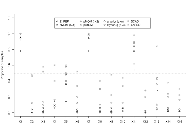
Figure 8: Proportions (across 50 simulated Nott-Kohn data sets) of instances in which each covariate was identified with a non-zero effect by the eight variable-selection and shrinkage methods under consideration.

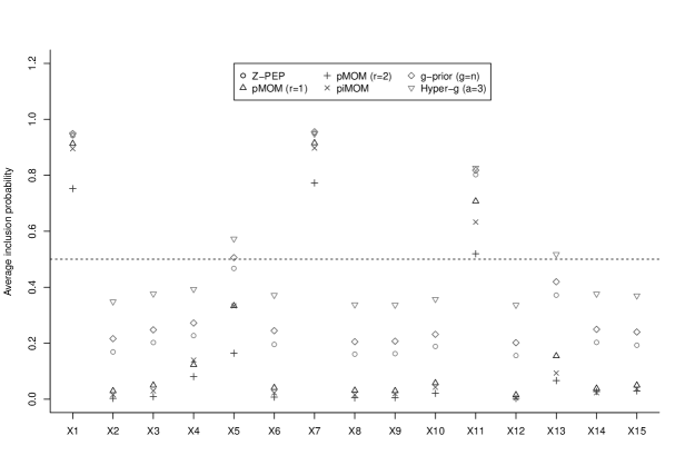
Figure 9: Averages of posterior inclusion probabilities (across 50 simulated Nott-Kohn samples) for the six variable-selection methods under consideration.

We also examined all eight of the methods compared here with respect to their variable-selection performance, in two ways: Figure 9 presents the proportions (across the 50 simulated Nott-Kohn data sets) of instances in which each covariate was identified with a non-zero effect (i.e., the cases where (a) the effect was not restricted to zero in the shrinkage methods and (b) the posterior inclusion probabilities were found to be greater than 0.5 in the variable-selection methods), and Figure 9 gives the mean posterior variable-inclusion probabilities across the 50 replicate data sets. In the following, we define the convention for each method that a variable is selected if either its proportion (Figure 9) or mean inclusion probability (Figure 9) exceeded 0.5. Under this convention, all methods did well in finding the “true” covariates $X_{1},X_{7}$ and $X_{11}$, and in avoiding selection of the “false” covariates $X_{2},X_{8},X_{9},X_{10},X_{12},X_{14}$ and $X_{15}$. Predictors $X_{5}$ and $X_{13}$, which are built into the data-generating model with smaller coefficients than those given to $X_{1}$ and $X_{7}$, were correctly selected only by the LASSO and the hyper-$g$ prior (in the case of $X_{5}$ and $X_{13}$) and the $g$-prior (in the case of $X_{5}$); covariates $X_{3},X_{4}$ and $X_{6}$, which have data-generating coefficients of 0 in the Nott-Kohn setting, were falsely selected by the LASSO and SCAD. Evidently the LASSO achieves its superior true-positive behavior in this case study only at the expense of an undesirably high false-positive rate. Z-PEP’s selection rates were nearly 50% for $X_{5}$ and 30–40% for $X_{13}$, making it competitive with (though somewhat inferior to) the hyper-$g$ prior and the $g$-prior on variable-selection behavior in this example, but (as noted above) this is balanced by Z-PEP’s better predictive performance.

6 Discussion

The major contribution of the research presented here is to simultaneously produce a minimally-informative prior and sharply diminish the effect of training samples on previously-studied expected-posterior-prior (EPP) methodology, resulting in a prior for variable selection in Gaussian regression models with very good variable-selection accuracy and excellent out-of-sample predictive behavior. As noted in the introduction, one of the main advantages of EPPs is that they achieve prior compatibility across models; the proposed prior in this paper also has this property (in contrast to other priors that have been developed in the Bayesian model selection literature, such as mixtures of $g$-priors), and in addition our prior has a unit-information structure and is robust to the size of the training sample. By combining ideas from the power-prior approach of Ibrahim and Chen (2000) and the unit-information prior of Kass and Wasserman (1995), we raise the likelihood involved in EPP to a power proportional to the inverse of the training sample size, resulting in prior information equivalent to one data point. In this way, with our power-expected-posterior (PEP) methodology, the effect of the training sample is minimal, regardless of its sample size, and we can choose training samples with size $n^{*}$ equal to the sample size $n$ of the original data, thus eliminating the need for training samples altogether. This choice promotes stability of the resulting Bayes factors, removes the arbitrariness arising from individual training-sample selections, and avoids the computational burden of averaging over many training samples. Additional advantages of our approach over methods that depend on training samples include the following.

• In variable-selection problems in linear models, the training data refer to both $y$ and $X$. Under the base-model approach (see Section 1.1), we can simulate training data $y^{*}$ directly from the prior predictive distribution of a reference model, but we still need to consider a subsample $X^{*}$ of the original design matrix $X$. The number of possible subsamples of $X$ can be enormous, inducing large variability, since some of those subsamples can be highly influential for the posterior analysis. By using our approach, and working with training-sample sizes equal to the size of the full data set, we avoid the selection of such subsamples by choosing $X^{*}=X$.

• The number $p$ of covariates in the full model is usually regarded as specifying the minimal training sample. This selection makes inference within the current data set coherent, but the size of the minimal training sample will change if additional covariates are added, meaning that the EPP distribution will depend incoherently on $p$. Moreover, if the data derive from a highly structured situation (such as an analysis of covariance in a factorial design), most choices of a small part of the data to act as a training sample would be untypical. Finally, the effect of the minimal training sample will be large in settings where the sample size $n$ is not much larger than $p$. This type of data set is common in settings (in disciplines such as bioinformatics and economics) in which (i) cases (rows in the data matrix) are expensive to obtain (bioinformatics) or limited by the number of available quarters of data (economics) but (ii) many covariates are inexpensive and readily available once the process of measuring the cases begins.

It is worth noting that our method, which is intended for settings in which there is a fixed covariate space of $p<n$ predictor variables, works in a totally different fashion than fractional Bayes factors. In the latter, the likelihood is partitioned based on two data subsets; one is used for building the prior within each model and the other is employed for model evaluation and comparison. In contrast, with our approach, the original likelihood is used only once, for simultaneous variable selection and posterior inference. Moreover, the fraction of the likelihood (power likelihood) — used in the expected-posterior expression of our prior distribution — refers solely to the imaginary data coming from a prior predictive distribution based on the reference model.

Our PEP approach can be implemented under any baseline prior choice; results using the $g$-prior and the independence Jeffreys prior as baseline choices are presented here. The conjugacy structure of the $g$-prior in Gaussian linear models makes calculations simpler and faster, and also offers flexibility in situations in which non-diffuse parametric prior information is available. When, by contrast, strong information about the parameters of the competing models external to the present data set is not available, the independence Jeffreys baseline prior can be viewed as a natural choice, and noticeable computational acceleration is provided by the fact that the posterior with the Jeffreys baseline is a special case of the posterior with the $g$-prior as baseline. In the Jeffreys case we have proven that the resulting variable-selection procedure is consistent; we conjecture that the same is true with the $g$-prior, but the proof has so far been elusive.

From our empirical results in two case studies — one involving simulated data, the other a real example based on the prediction of air pollution levels from meteorological covariates — we conclude that our method

• is systematically more parsimonious (under either baseline prior choice) than the EPP approach using the Jeffreys prior as a baseline prior and minimal training samples, while sacrificing no desirable performance characteristics to achieve this parsimony;

• is robust to the size of the training sample, thus supporting the use of the entire data set as a “training sample” — thereby eliminating the need for random sampling over different training sub-samples, which promotes inferential stability and fast computation;

• identifies maximum a-posteriori models that achieve better out-of-sample predictive performance than that attained by a wide variety of previously-studied variable-selection and coefficient-shrinkage methods, including standard EPPs, the $g$-prior, the hyper-$g$ prior, non-local priors, the LASSO and SCAD; and

• has low impact on the posterior distribution even when $n$ is not much larger than $p$.

Our PEP approach could be applied to any prior distribution that is defined via imaginary training samples. Additional future extensions of our method include implementation in generalized linear models, where computation is more demanding.

Supplementary material

The Appendix is available in a web supplement at ***.

Abbreviations used in the paper

BIC = Bayesian information criterion, EIBF = expected intrinsic Bayes factor, EPP = expected-posterior prior, IBF = intrinsic Bayes factor, J-EPP = EPP with Jeffreys baseline prior, J-PEP = PEP prior with Jeffreys-prior baseline, LASSO = least absolute shrinkage and selection operator, PEP = power-expected-posterior, Z-PEP = PEP prior with Zellner $g$-prior baseline, SCAD = smoothly-clipped absolute deviations.

References

- (1)
- Aitkin (1991) Aitkin, M. (1991), ‘Posterior Bayes factors’, Journal of the Royal Statistical Society B, 53, 111–142.
- Barbieri and Berger (2004) Barbieri, M. and Berger, J. (2004), ‘Optimal predictive model selection’, Annals of Statistics, 32, 870–897.
- Berger and Pericchi (1996a) Berger, J. and Pericchi, L. (1996a), The intrinsic Bayes factor for linear models, in ‘Bayesian Statistics (Volume 5)’, J. Bernardo, J. Berger, A. Dawid, and A. Smith, eds., Oxford University Press, pp. 25–44.
- Berger and Pericchi (1996b) Berger, J. and Pericchi, L. (1996b), ‘The intrinsic Bayes factor for model selection and prediction’, Journal of the American Statistical Association, 91, 109–122.
- Berger and Pericchi (2004) Berger, J. and Pericchi, L. (2004), ‘Training samples in objective model selection’, Annals of Statistics, 32, 841–869.
- Breiman and Friedman (1985) Breiman, L. and Friedman, J. (1985), ‘Estimating optimal transformations for multiple regression and correlation’, Journal of the American Statistical Association, 80, 580–598.
- Casella et al. (2009) Casella, G., Girón, F., Martínez, M. and Moreno, E. (2009), ‘Consistency of Bayesian procedures for variable selection’, Annals of Statistics, 37, 1207–1228.
- Casella and Moreno (2006) Casella, G. and Moreno, E. (2006), ‘Objective Bayesian variable selection’, Journal of the American Statistical Association, 101, 157–167.
- Consonni and Veronese (2008) Consonni, G. and Veronese, P. (2008), ‘Compatibility of prior specifications across linear models’, Statistical Science, 23, 332–353.
- Council (2005) Council, N. R. (2005), Mathematics and 21st Century Biology, Committee on Mathematical Sciences Research for Computational Biology, The National Academies Press.
- Fan and Li (2001) Fan, J. and Li, R. (2001), ‘Variable selection via nonconcave penalized likelihood and its oracle properties’, Journal of the American Statistical Association, 96, 1348–1360.
- Fouskakis and Ntzoufras (2013a) Fouskakis, D. and Ntzoufras, I. (2013a), ‘Computation for intrinsic variable selection in normal regression models via expected-posterior prior’, Statistics and Computing 23, 491–499.
- Fouskakis and Ntzoufras (2013b) Fouskakis, D. and Ntzoufras, I. (2013b), Limiting behavior of the Jeffreys Power-Expected-Posterior Bayes factor in Gaussian linear models, Technical report, Department of Mathematics, National Technical University of Athens.
- Girón et al. (2006) Girón, F., Martínez, M., Moreno, E. and Torres, F. (2006), ‘Objective testing procedures in linear models: Calibration of the p-values’, Scandinavian Journal of Statistics, 33, 765–784.
- Good (2004) Good, I. (2004), Probability and the Weighting of Evidence, Haffner, New York, USA.
- Ibrahim and Chen (2000) Ibrahim, J. and Chen, M. (2000), ‘Power prior distributions for regression models’, Statistical Science, 15, 46–60.
- Iwaki (1997) Iwaki, K. (1997), ‘Posterior expected marginal likelihood for testing hypotheses’, Journal of Economics, Asia University, 21, 105–134.
- Johnson and Rossell (2010) Johnson, V. and Rossell, D. (2010), ‘On the use of non-local prior densities in Bayesian hypothesis tests’, Journal of the Royal Statistical Society B, 72, 143–170.
- Johnson and Rossell (2012) Johnson, V. and Rossell, D. (2012), ‘Bayesian model selection in high-dimensional settings’, Journal of the American Statistical Association, 107, 649–660.
- Johnstone and Titterington (2009) Johnstone, I. M. and Titterington, M. (2009), ‘Statistical challenges of high-dimensional data’, Philosophical Transactions of the Royal Society A, 367, 4237–4253.
- Kass and Wasserman (1995) Kass, R. and Wasserman, L. (1995), ‘A reference Bayesian test for nested hypotheses and its relationship to the Schwarz criterion’, Journal of the American Statistical Association, 90, 928–934.
- Liang et al. (2008) Liang, F., Paulo, R., Molina, G., Clyde, M. and Berger, J. (2008), ‘Mixtures of g priors for Bayesian variable selection’, Journal of the American Statistical Association, 103, 410–423.
- Moreno and Girón (2008) Moreno, E. and Girón, F. (2008), ‘Comparison of Bayesian objective procedures for variable selection in linear regression’, Test, 17, 472–490.
- Moreno et al. (2003) Moreno, E., Girón, F. and Torres, F. (2003), ‘Intrinsic priors for hypothesis testing in normal regression models’, Revista de la Real Academia de Ciencias Exactas, Fisicas y Naturales. Serie A. Matematicas, 97, 53–61.
- Nott and Kohn (2005) Nott, D. and Kohn, R. (2005), ‘Adaptive sampling for Bayesian variable selection’, Biometrika, 92, 747–763.
- O’Hagan (1995) O’Hagan, A. (1995), ‘Fractional Bayes factors for model comparison’, Journal of the Royal Statistical Society B, 57, 99–138.
- Pérez (1998) Pérez, J. (1998), Development of Expected Posterior Prior Distribution for Model Comparisons, PhD thesis, Department of Statistics, Purdue University, USA.
- Pérez and Berger (2002) Pérez, J. and Berger, J. (2002), ‘Expected-posterior prior distributions for model selection’, Biometrika, 89, 491–511.
- Schwarz (1978) Schwarz, G. (1978), ‘Estimating the dimension of a model’, Annals of Statistics, 6, 461–464.
- Spiegelhalter et al. (2004) Spiegelhalter, D., Abrams, K. and Myles, J. (2004), Bayesian Approaches to Clinical Trials and Health-Care Evaluation, Statistics in Practice, Wiley, Chichester, UK.
- Spiegelhalter and Smith (1988) Spiegelhalter, D. and Smith, A. (1988), ‘Bayes factors for linear and log-linear models with vague prior information’, Journal of the Royal Statistical Society B, 44, 377–387.
- Tibshirani (1996) Tibshirani, R. (1996), ‘Regression shrinkage and selection via the lasso’, Journal of the Royal Statistical Society B, 58, 267–288.
- Womack et al. (2014) Womack, A., Novelo, L. and Casella, G. (2014), ‘Inference from intrinsic Bayes’ procedures under model selection and uncertainty’, Journal of the American Statistical Association, forthcoming .
- Zellner (1976) Zellner, A. (1976), “Bayesian and non-Bayesian analysis of the regression model with multivariate Student-t error terms”, Journal of the American Statistical Association, 71, 400–405.