Testing experiments on synchronized Petri nets

Abstract

Synchronizing sequences have been proposed in the late 60’s to solve testing problems on systems modeled by finite state machines. Such sequences lead a system, seen as a black box, from an unknown current state to a known final one.

This paper presents a first investigation of the computation of synchronizing sequences for systems modeled by bounded synchronized Petri nets. In the first part of the paper, existing techniques for automata are adapted to this new setting. Later on, new approaches, that exploit the net structure to efficiently compute synchronizing sequences without an exhaustive enumeration of the state space, are presented.

I Introduction

Due to increasingly larger size and rising complexity, the need of checking systems’ performance increases and testing problems periodically resurface.

These problems have been introduced by the pioneering paper of Moore [moore56], where the main focus is to understand what can be inferred about the internal conditions of a system under test from external experiments. In his gedanken-experiment, the system under investigation is a fixed semi-automaton seen as a black box. Lee and Yannakakis [Lee-survey] have widely reviewed those problems and the techniques to solve them. They have stated five fundamental problems of testing: i) determining the final state after a test; ii) state identification; iii) state verification; iv) conformance testing; v) machine identification. Among these, the problem of determining the final state after a test is considered. This problem has been addressed and essentially completely solved using Mealy machines around 1960, using homing sequences (HS) and synchronizing sequences (SS).

The synchronization problem is the problem the reader deals with in this work. It concerns how to drive a system to a known state when its current state it is not known and when the outputs are not observable. This problem has many important applications and is of general interest. It is of relevant importance for robotics and robotic manipulation [Natarajan86, Natarajan89, ananichev2003], when dealing with part handling and orienting problems in industrial automation such as part feeding, loading, assembly and packing. The reader can easily see that for example every device part, when arriving at manufacturing sites, needs to be sorted and oriented before assembly. Synchronization protocols have been developed to address global resource sharing in hierarchical real-time scheduling frameworks [Heuvel99, Behnam_07]. An interesting automotive application can be found in [Nolte09]. Synchronization experiments have been done also in biocomputing, where Benenson et al. [Benenson01, Benenson03] have used DNA molecules as both software and hardware for finite automata of nano-scaling size. They have produced a solution of $3\times 10^{12}$ identical automata working in parallel. In order to synchronously bring each automaton to its ”ready-to-restart” state, they have spiced it with a DNA molecule whose nucleotide sequence encodes a reset word. Jürgensen [Jurgensen2008] has surveyed synchronization issues from the point of view of coding theory in real life communication systems. He has presented the concept of synchronization in information channels, both in the absence and in the presence of noise. Synchronization is an important issue in network time protocol [Gaderer10, Mills91], where sharing of time information guaranties the correct internet system functioning. Most of real systems, natural or man-built, have no integrated reset or cannot be equipped with. That is the case of digital circuits, where a reset circuit not only involves human intervention but increases the cost of the device itself reducing its effectiveness. In this field Cho et al. [Cho93] have shown how to generate test cases for synchronous circuits with no reset. When classic procedures fail due to large circuit size or because a synchronizing sequence does not exist, Lu et al. [Pomeranz96] propose a technique based on partial reset, i.e., special inputs that reset a subset of the flip-flops in the circuit leaving the other flip-flops at their current values. Hierons [Hierons04] has presented a method to produce a test sequence with the minimum number of resets. Nowadays the synchronizing theory is a field of very intensive research, motivated also by the famous C̆erný conjecture [cernia64]. In 1964 Ján C̆erný has conjectured that $(n-1)^{2}$ is the upper bound for the length of the shortest SS for any $n-$state machine. The conjecture is still open except for some special cases [eppstein90],[ananichev2003],[trahtman90]. Synchronization allows simple error recovery since, if an error is detected, a SS can be used to initialize the machine into a known state. That is why synchronization plays a key rôle in scientific contexts, without which all system behavior observations may become meaningless. Thus the problem of determining which conditions admit a synchronization is an interesting challenge. This is the case of the road coloring problem, where one is asked whether there exists a coloring, i.e., an edge labeling, such that the resulting automaton can be synchronized. It was first stated by Adler in [Adler77]. It has been investigated in various special cases and finally a positive solution has been presented by Trahtman in [Trahtman09], for which complexity analysis are provided [Roman11].

At present the problem of determining a synchronizing sequence has not yet been investigated for Petri net (PN) models and only few works have addressed the broad area of testing in the PN framework.

The question of automatically testing PNs has been investigated by Jourdan and Bochmann in [JourdanBochmann09]. They have adapted methods originally developed for Finite State Machines (FSMs) and, classifying the possible occurring types of error, identified some cases where free choice and $1$-safe PNs [Murata] provide more significant results especially in concurrent systems. Later the authors have extended their results also to $k$-safe PNs [Bochmann09]. Zhu and He have given an interesting classification of testing criteria [ZhuHe02] — without testing algorithms — and presented a theory of testing high-level Petri nets by adapting some of their general results in testing concurrent software systems.

In the PN modeling framework, one of the main supervisory control tasks is to guide the system from a given initial marking to a desired one similarly to the synchronization problem. Yamalidou et al. have presented a formulation based on linear optimization [Yamalidou91, Yamalidou92]. Giua et al. have investigated the state estimation problem, proposing an algorithm to calculate an estimate — and a corresponding error bound — for the actual marking of a given PN based on the observation of a word. A different state estimation approach has been presented by Corona et al. [Giuaseatzu07], for labelled PNs with silent transitions, i.e., transitions that do not produce any observation. Similar techniques have been proposed by Lingxi et al. in [Lingxi09] to get a minimum estimate of initial markings, aiming to characterize the minimum number of resources required at the initialization for a variety of systems.

This paper is focused on bounded synchronized PNs and the SS problem here is first investigated. The paper shows how the Mealy machine approach [Lee-survey] can be easily adapted to systems represented by the class of bounded synchronized PNs. Synchronized PNs, as introduced by Moalla et al. in [Moalla78], are nets where a label associated with each transition corresponds to an external input event whose occurrence causes the firing of all marking enabled transitions having this label. Note that SSs are independent of the output and this makes the synchronized PN a suitable model for such an analysis. Then the authors consider a special class of Petri nets called state machines (SMs) [Murata], characterized by the fact that each transition has a single input and a single output arc. Note that this model, albeit simple, is more general an automaton. In fact, while the reachability graph of a state machine with a single token is isomorphic — assuming all places can be marked — to the net itself, as the number of tokens $k$ in the net increases the reachability graph grows as $k^{m-1}$, where $m$ is the number of places in the net. It is shown that for strongly connected SM even in the case of multiple tokens, the existence of SS can be efficiently determined by just looking at the net structure, thus avoiding the state explosion problem. These results are also extended to SMs that are not strongly connected and to PN containing SM subnets. The effectiveness of the technique is proved via a toolbox we developed on Matlab [Pocciweb].

The paper is organized as follows. In Section II the background on automata with inputs and PNs is provided. Section III presents the classic SS construction method for automata with inputs. Section IV shows how to obtain SSs by adapting the classic method developed for automata with inputs to bounded synchronized PNs, via reachability graph construction. Section LABEL:SMPN proposes an original technique, based on path analysis, for efficiently determining SSs on strongly connected SMs. Section LABEL:complexity presents a short discussion of algorithm complexity. The case of non-strongly connected SMs is investigated in Section LABEL:NSCPN. In Section LABEL:sec:subSMs our approaches are extended to nets containing state machine subnets. In Section LABEL:sec:ex_results numerical results are presented, applying our tool to randomly generated SMs. Finally, in Section LABEL:conclusion, conclusions are drawn and open areas of research are outlined.

II Background

II-A Automata with inputs

An automaton with inputs $\Lambda$ is a structure

$$\Lambda=(\chi,E,\delta),$$

where $\chi$ and $E$ are finite and nonempty sets of states and input events respectively, and $\delta:\chi\times E\rightarrow\chi$ is the state transition function.

When the automaton is in the current state $x\in\chi$ and receives an event $e\in E$, it reaches the next state specified by $\delta(x,e)$.

Note that $\delta$ is usually assumed to be a total function, i.e., a function defined on each element $(x,e)$ of its domain. In such a case the automaton is called completely specified.

The number of states and input events are respectively denoted by $n=|\chi|$, $p=|E|$. One can extend the transition function $\delta$ from input events to sequences of input events as follows: a) if $\varepsilon$ denotes the empty input sequence, $\delta(x,\varepsilon)=x$ for all $x\in\chi$; b) for all $e\in E$ and for all $w\in E^{*}$ it holds that $\delta(x,we)=\delta(\delta(x,w),e)$.

The transition function $\delta$ can also be extended to a set of states as follows: for a set of states $\chi^{\prime}\subseteq\chi$, an input event $e\in E$ yields the set of states $\chi^{\prime\prime}=\delta(\chi^{\prime},e)=\bigcup_{x\in\chi^{\prime}}\delta(x,e).$

A simple way to represent any automaton is a graph, where states and input events are respectively depicted as nodes and labelled arcs.

An automaton with inputs is said strongly connected if there exists a directed path from any node of its graph to any other node.

The set of nodes of a non-strongly connected automaton can be partitioned into its maximal strongly connected components. A component is called ergodic, if its set of output arcs is included in its set of input arcs, transient, otherwise.

An automaton contains at least one ergodic component and a strongly connected automaton consists of a single ergodic component.

II-B Place/Transition nets

In this section, it is recalled the PN formalism used in the paper. For more details on PNs the reader is referred to [Murata, BODavid04].

A Petri net (PN), or more properly a Place/Transition net, is a structure

$$N=\left(P,T,Pre,Post\right),$$

where $P$ is the set of $m$ places, $T$ is the set of $q$ transitions, $Pre:\,P\times T\rightarrow\mathbb{N}$ and $Post:\,P\times T\rightarrow\mathbb{N}$ are the pre and post incidence functions that specify the weighted arcs.

A marking is a vector $M:\,P\rightarrow\mathbb{N}$ that assigns to each place a nonnegative integer number of tokens; the marking of a place $p$ is denoted with $M(p)$. A marked PN is denoted $\langle N,M_{0}\rangle$.

A transition $t$ is enabled at $M$ iff $M\geq Pre(\cdot,t)$. An enabled transition may be fired yielding the marking $M^{\prime}=M+Post(\cdot,t)-Pre(\cdot,t)$. The set of enabled transitions at $M$ is denoted ${\cal E}(M)$.

$M[\sigma\rangle$ denotes that the sequence of transitions $\sigma=t_{1}\ldots t_{k}$ is enabled at $M$ and $M[\sigma\rangle M^{\prime}$ denotes that the firing of $\sigma$ from $M$ yields $M^{\prime}$.

A marking $M$ is said to be reachable in $\langle N,M_{0}\rangle$ iff there exists a firing sequence $\sigma$ such that $M_{0}[\sigma\rangle M$. The set of all markings reachable from $M_{0}$ defines the reachability set of $\langle N,M_{0}\rangle$ and is denoted with $R(N,M_{0})$.

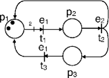
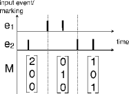
Figure 1: A synchronized PN (a) and a possible behavior (b).

The $preset$ and $postset$ of a place $p$ are respectively denoted ${}^{\bullet}p$ and $p^{\bullet}$. One can define the set of input transitions for a set of places $\hat{P}$ as the set ${}^{\bullet}\hat{P}=\{t:\forall p\in\hat{P},\ t\in\ ^{\bullet}{p}\}$. Analogously the set of output transitions for a set of places $\hat{P}$ is the set $\hat{P}^{\bullet}=\{t:\forall p\in\hat{P},\ t\in\ {p}^{\bullet}\}$.

II-C Synchronized Petri nets

A synchronized PN [BODavid04] is a structure $\langle N,E,f\rangle$ such that: i) $N$ is a P/T net; ii) $E$ is an input alphabet of external events; iii) $f:T\to E$ is a labeling function that associates with each transition $t$ an input event $f(t)$.

Given an initial marking $M_{0}$, a marked synchronized PN is a structure $\langle N,M_{0},E,f\rangle$.

One extends the labeling function to sequences of transitions as follows: if $\sigma=t_{1}t_{2}\ldots t_{k}$ then $f^{*}(\sigma)=f(t_{1})f(t_{2})\ldots f(t_{k})$.

The set $T_{e}$ of transitions associated with input event $e$ is defined as follows: $T_{e}=\{t\mid\;t\in T,f(t)=e\}$. Equivalently all transitions in $T_{e}$ are said to be receptive to input event $e$.

The evolution of a synchronized PN is driven by input sequences as it follows. At marking $M$, transition $t\in T$ is fired iff:

1. it is enabled, i.e., $t\in{\cal E}(M)$;

2. the event $e=f(t)$ occurs.

On the contrary, the occurrence of an event associated with a transition $t\not\in{\cal E}(M)$ does not produce any firing. Note that a single server semantic is here adopted, i.e., when input event $e$ occurs, the enabled transitions in $T_{e}$ fire only once regardless of their enabling degree.

One writes $M\xrightarrow{w}M^{\prime}$ to denote the fact that the application of input event sequence $w=e_{1}\ldots e_{k}$ from $M$ drives the net to $M^{\prime}$.

In Figure 1 is shown an example of synchronized PN. Note that labels next to each transition denote its name and the associated input event. In Figure 1 the net evolution is presented over a possible input sequence $w=e_{2}e_{1}e_{1}e_{2}e_{2}$ starting from marking $M_{0}$.

In the rest of the paper, the reader will only deal with the class of bounded synchronized PNs that also satisfy the following structural restriction, that is common in the literature to ensure the determinism of the model:

$$\nexists p\;s.t.\qquad t,t^{\prime}\in p^{\bullet}\;and\;f(t)=f(t^{\prime}).$$ (1)

When an event occurs in a deterministic net, all enabled transitions receptive to that event can simultaneously fire. Thus an input sequence $w=e_{1}e_{2}\cdots e_{k}\in E^{*}$ drives a deterministic net through the sequence of markings $M_{0}$, $M_{1}$, $M_{2}$, $\cdots$, $M_{k}$ where $M_{0}$ is the initial marking and

$$M_{i+1}=M_{i}+\sum_{t\in T_{e_{i+1}}\bigcap{\cal E}(M_{i})}\left(Post(\cdot,t)-Pre(\cdot,t)\right).$$

Example 1

Consider the PN of Figure 1 and let $M=[2\,0\,1]^{T}$ be the current marking. Transitions $t_{1}$ and $t_{3}$ are enabled and upon the occurrence of event $e_{1}$ will simultaneously fire, yielding marking $M^{\prime}=[1\,1\,0]^{T}$. Note that markings $[0\,1\,1]^{T}$ and $[3\,0\,0]^{T}$, respectively obtained by the independent firing of $t_{1}$ and $t_{3}$, are never reachable. $\blacksquare$

A marked PN $\langle N,M_{0}\rangle$ is said to be bounded if there exists a positive constant $k$ such that for all $M\in R(N,M_{0})$, $M(p)\leq k\,\,\forall p\in P$. Such a net has a finite reachability set. In this case, the behavior of the net can be represented by the reachability graph (RG), a directed graph whose vertices correspond to reachable markings and whose edges correspond to the transitions and the associated event causing a change of marking.

The graph in Figure 3 (disregarding the dashed edges) is the reachability graph of the PN in Figure 1.

II-D State machine Petri nets

Let first recall the definition of a state machine PN.

Definition 2 (State machine PN)

[Murata] A state machine (SM) PN is an ordinary PN such that each transition $t$ has exactly one input place and exactly one output place, i.e.,

$$\hskip 69.70915pt|^{\bullet}t|=|t^{\bullet}|=1\qquad(\forall t\in T)\hskip 69.70915pt\blacksquare$$

Observe that a SM $N=\left(P,T,Pre,Post\right)$ may also be represented by an associated graph ${\cal G}_{N}=(V,A)$ whose set of vertices $V=P$ coincides with set of places of the net, and whose set of arcs $A$ corresponds to the set of transitions of the net, i.e., $A\subseteq P\times P=\{(p_{i},p_{j})\mid\exists t\in T,p_{i}={{}^{\bullet}t},p_{j}=t^{\bullet}\}.$

Such a graph can be partitioned into its maximal strongly connected components, analogously to the automata with inputs. These components induce also a partition of the set of places of the corresponding SM.

Definition 3 (Associated graph)

Given a SM $N=\left(P,T,Pre,Post\right)$, let ${\cal G}_{N}=(P,A)$ be its associated graph. $P$ can be partitioned into components as follows:

$$P=P_{1}\cupdot\cdots\cupdot P_{k}$$

such that for all $i=1,\ldots,k$ and $A_{i}=A\cap(P_{i}\times P_{i})$ it holds that $(P_{i},A_{i})$ is a maximal strongly connected sub-graph of ${\cal G}_{N}$. $\blacksquare$

As discussed in Section II-A, components $P_{1},\ldots P_{k}$ can be classified as transient or ergodic components.

Definition 4 (Condensed graph)

Given a SM $N=(P,T,$ $Pre,Post)$, its corresponding condensed graph ${\cal C}(N)$ is defined as a graph where each node represents a maximal strongly connected component and whose edges represent the transitions connecting these components. $\blacksquare$

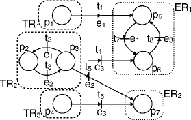
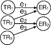
Figure 2: A not strongly connected PN (a) and its condensed graph (b).

In Figure 2 it is shown an example of a synchronized SM which is not strongly connected. Transient and ergodic components are respectively identified by dashed and dotted boxes. For such a net the transient components are $TR_{1}=\{p_{1}\}$, $TR_{2}=\{p_{2},\ p_{3}\}$, $TR_{3}=\{p_{4}\}$ and the ergodic components are $ER_{1}=\{p_{5},\ p_{6}\}$ and $ER_{2}=\{p_{7}\}$. The corresponding ${\cal C}(N)$ is shown in Figure 2, where subnets induced by each component are represented by single nodes.

III Synchronizing sequences for automata with inputs

In this section, the SS classic construction is presented by the aid of finite automata.

Definition 5 (SSs on automata)

Consider an automaton with inputs $\Lambda=(\chi,E,\delta)$ and a state $\bar{x}\in\chi$. The input sequence $\bar{w}$ is called synchronizing for state $\bar{x}$ if it drives the automaton to $\bar{x}$, regardless of the initial state, i.e., $\forall x\in\chi$ it holds that $\delta(x,w)=\bar{x}$. $\blacksquare$

The information about the current state of $\Lambda$ after applying an input sequence $w$ is defined by the set $\phi(w)=\delta(\chi,w)$, called the current state uncertainty of $w$. In other words $w$ is a synchronizing sequence (SS) that takes the automaton to the final state $\bar{x}$ iff $\phi(w)=\{\bar{x}\}$.

The synchronizing tree method [Hennie68, kohavi2] has been proposed to provide shortest SSs. Such a method is suitable only for small size systems, since the memory required to build up the tree is high, and becomes useless when the size grows. As a matter of fact the problem of finding shortest SSs is known to be NP-complete [eppstein90].

Two polynomial algorithms have been mainly used to provide SSs that are not necessarily the shortest. The so-called greedy and cycle algorithms, respectively of Eppstein [eppstein90] and Trahtman [trahtman04], that have equivalent complexity.

The greedy algorithm [eppstein90] determines an input sequence that takes a given automaton, regardless of its initial state, to a known target state: note that the target state is determined by the algorithm and cannot be specified by the user. Here we propose a slightly different implementation of the greedy algorithm (see Algorithm 7), that takes as input also a state $\bar{x}$ and determines a sequence that synchronizes to that state.

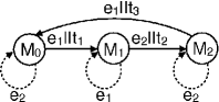
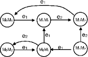
Figure 3: The completely specified RG (a) and the corresponding auxiliary graph (b) of the PN in Figure 1.

This algorithm is later used as a building block to determine a SS to reach a given marking among those in the reachability set of a bounded PN.

Definition 6 (Auxiliary graph)

Given an automaton with inputs $\Lambda$ with $n$ states, let ${\cal A}(\Lambda)$ be its auxiliary graph. ${\cal A}(\Lambda)$ contains $n(n+1)/2$ nodes, one for every unordered pair $(x^{\prime},x^{\prime\prime})$ of states of $\Lambda$, including pairs $(x,x)$ of identical states. There exists an edge from node $(x^{\prime},x^{\prime\prime})$ to $(\hat{x}^{\prime},\hat{x}^{\prime\prime})$ labeled with an input event $e\in E$ iff $\delta(x^{\prime},e)=\hat{x}^{\prime}$ and $\delta(x^{\prime\prime},e)=\hat{x}^{\prime\prime}$.                    $\blacksquare$

Algorithm 7

(Greedy computation of SSs on automata with inputs)
Input: An auxiliary graph ${\cal A}(\Lambda)$, associated with an automaton with inputs $\Lambda=(\chi,E,\delta)$, and a target state $\bar{x}\in\chi$.
Ouput: A SS $\bar{w}$ for state $\bar{x}$.

1. Let $i=0$.

2. Let $w_{0}=\varepsilon$, the empty initial input sequence.

3. Let $\phi(w_{0})=\chi$, the initial current state uncertainty.

4. While $\phi(w_{i})\neq\{\bar{x}\}$, do

   1. $i=i+1$.

   2. Pick two states $x,x^{\prime}\in\phi(w_{i-1})$ such that $x\neq x^{\prime}$.

   3. If there does not exist any path in ${\cal A}(\Lambda)$ from node $(x^{\prime},x^{\prime\prime})$ to $(\bar{x},\bar{x})$, stop the computation, there exists no SS for $\bar{x}$.

   4. Else find the shortest path from node $(x^{\prime},x^{\prime\prime})$ to $(\bar{x},\bar{x})$ and let $w$ be the input sequence along this path, do

      1. 4.3.1. $w_{i}=w_{i-1}w$

      2. 4.3.2. $\phi(w_{i})=\delta(\phi(w_{i-1}),w)$.

5. $\bar{w}=w_{i}$. $\blacksquare$

The following theorem provides a necessary and sufficient condition for the existence of a SS for a target final state.

Theorem 8

The following three propositions are equivalent.

1. Given an automaton with inputs $\Lambda=(\chi,E,\delta)$, there exists a SS for state $\bar{x}\in\chi$;

2. ${\cal A}(\Lambda)$ contains a path from every node $(x^{\prime},x^{\prime\prime})$, where $x^{\prime},x^{\prime\prime}\in\chi$, to node $(\bar{x},\bar{x})$;

3. Algorithm 7 determines a SS $\bar{w}$ for state $\bar{x}\in\chi$ at step 5., if there exists any SS.

$M_{0}$	$[2\,0\,0]^{T}$
$M_{1}$	$[0\,1\,0]^{T}$
$M_{2}$	$[1\,0\,1]^{T}$

Table I: Markings of the PN in Figure 1.

Proof:

[1) implies 2)] If there exists a SS for state $\bar{x}\in\chi$, there exists an input sequence ${w}$ for $\bar{x}$ s.t. for any $x^{\prime},x^{\prime\prime}\in\chi$ it holds that $\delta(x^{\prime},{w})=\delta(x^{\prime\prime},{w})=\bar{x}$. Hence there exists a path labeled ${w}$ from any $(x^{\prime},x^{\prime\prime})$ to $(\bar{x},\bar{x})$.

[2) implies 3)] Consider iteration $i$ of the while loop of Algorithm 7. If there exists a path labeled $w$ from any $(x^{\prime},x^{\prime\prime})$ to $(\bar{x},\bar{x})$, then it holds that $\delta(\{x^{\prime},x^{\prime\prime}\},w)=\{\bar{x}\}$. Hence the following inequality holds:

$$|\phi(w_{i})|=|\delta(\phi(w_{i-1})\backslash\{x,x^{\prime}\},w)\cup\{\bar{x}\}|\leq|\phi(w_{i})|-1.$$

The existence of such a sequence for every couple of states $x^{\prime},x^{\prime\prime}\in\chi$ assures that the current state uncertainty will be reduced to singleton $\{\bar{x}\}$ after no more than $n$ iteration.

[3) implies 1)] Since Algorithm 7 requires the current state uncertainty to be singleton and uses it as a stop criterium, if it terminates at step 5., then the sequence found is clearly a SS. $\square$

One can easily understand that, when the automaton is not strongly connected, the above reachability condition will be verified only when there exists only one ergodic component and there may exist a SS only for those states belonging to this ergodic component.

IV Synchronizing sequences for bounded synchronized PNs

When computing a SS for real systems modeled by automata, it is assumed that a complete description of the model in terms of space-set, input events and transition function is given. The idea is that the test generator knows all possible states in which the system may be.

A similar notion can be given for Petri nets, where equivalently one can say that the test generator knows a ”starting state”, i.e., a possible state, of the system and the initial uncertainty coincides with the set of states reachable from this starting state.

In a synchronization problem via PNs, it is given a Petri net $N$ and a starting marking $M_{0}$. The current marking $M$ is unknown, but it is assumed to be reachable from $M_{0}$.

This starting marking, together with the firing rules, provides a characterization of the initial state uncertainty, given by ${\cal M}_{0}=R(N,M_{0})$. The goal is to find an input sequence that, regardless of the initial marking, drives the net to a known marking $\bar{M}\in R(N,M_{0})$.

Given a synchronized PN $\langle N,E,f\rangle$, a straightforward approach to determine a SS consists in adapting the existing approach for automata to the reachability graph (RG).

It is easy to verify that this direct adaptation presents one shortcoming that makes it not always applicable: the greedy approach requires the graph to be completely specified, while in a RG of a PN this condition is not always true. In fact, from a marking not all transitions are necessarily enabled, causing the RG of the PN to be partially specified. In order to use the aforementioned approach it is necessary to turn its RG ${\cal G}$ into a completely specified $\tilde{\cal G}$.

Example 9

Consider the PN in Figure 1. The current marking $M=[2\ 0\ 0]^{T}$ enables only transition $t_{1}$, then all events not associated with $t_{1}$ are not specified. Hence for that marking one adds a self loop labelled $e_{2}$ and so on for the rest of the reachable markings. $\blacksquare$

In Figure 3 is shown the RG of the PN in Figure 1. Note that dashed edges are added in order to make it completely specified. In Figure 3 is shown the corresponding auxiliary graph of the RG in Figure 3.

One can summarize the modified approach for PNs in the following algorithm.

Algorithm 10

(RG computation of SSs on synchronized PNs)
Input: A bounded synchronized PN $\langle N,E,f\rangle$, a starting marking $M_{0}$ and a target marking $\bar{M}$.
Ouput: A SS $\bar{w}$ for marking $\bar{M}\in R(N,M_{0})$.

1. Let ${\cal G}$ be the reachability graph of $\langle N,M_{0}\rangle$.

2. Let $\tilde{\cal G}$ be the modified reachability graph obtained by completing ${\cal G}$, then by adding a self loop labelled $e$, i.e., $\forall M\in{\cal G}$ and $\forall e\in E$ s.t. $\nexists t\in T_{e}\cap{\cal E}(M)$.

3. Construct the corresponding auxiliary graph ${\cal A}(\tilde{\cal G})$.

4. A SS for marking $\bar{M}$, if such a sequence exists, is given by the direct application of Algorithm 7 to ${\cal A}(\tilde{\cal G})$, having $\bar{M}$ as target. $\blacksquare$

The following proposition can now be stated.

Proposition 11

Given a bounded synchronized PN $N$ and a starting marking $M_{0}$, there exists a SS leading to a marking $\bar{M}\in R(N,M_{0})$ iff the reachability condition on its auxiliary graph ${\cal A}(\tilde{\cal G})$ is verified, i.e., there is a path from every node $(M_{i},M_{j})$, with $M_{i},M_{j}\in R(N,M_{0})$, to node $(\bar{M},\bar{M})$.