Abstract

We show that it is possible to accommodate physical scalar resonances within a minimal nonlinearly realized electroweak theory in a way compatible with a natural Hopf algebra selection criterion (Weak Power Counting) and the relevant functional identities of the model (Local Functional Equation, Slavnov-Taylor identity, ghost equations, b-equations). The Beyond-the-Standard-Model (BSM) sector of the theory is studied by BRST techniques. The presence of a mass generation mechanism à la Stückelberg allows for two mass invariants in the gauge boson sector. The corresponding ’t Hooft gauge-fixing is constructed by respecting all the symmetries of the theory. The model interpolates between the Higgs and a purely Stückelberg scenario. Despite the presence of physical scalar resonances, we show that tree-level violation of unitarity in the scattering of longitudinally polarized charged gauge bosons occurs at sufficiently high energies, if a fraction of the mass is generated by the Stückelberg mechanism. The formal properties of the physically favoured limit after LHC7-8 data, where BSM effects are small and custodial symmetry in the gauge boson sector is respected, are studied.

1 Introduction

The discovery in 2012 of a physical scalar resonance by the LHC experiments ATLAS and CMS [1, 2] has paved the way to the experimental verification of the electroweak spontaneous symmetry breaking (SSB) mechanism realized in Nature.

Recent fits based on the LHC7-8 results [3, 4] are compatible with the identification of the newly discovered scalar resonance with the Standard Model (SM) Higgs boson. Electroweak SSB might therefore occur through the simplest linear Higgs mechanism.

A well-known alternative to the mass generation of elementary particles, which does not rely on the existence of fundamental scalars, is the Stückelberg mechanism [5, 6]. Being based on a nonlinearly realized non-Abelian gauge symmetry, the mass generation à la Stückelberg yields non-renormalizable models that are usually treated as an effective low energy approximation to a more fundamental theory [7]. They can be used as a tool for describing possible beyond-the-SM (BSM) effects [8].

In order to ascertain the nature of electroweak SSB, it is important to establish whether the existence of a Stückelberg mass component can be already excluded by using the current LHC data. This problem can be conveniently formulated within a recently proposed model [9], where the mass generation happens via the Stückelberg mechanism and nonetheless a set of physical scalar resonances exist.

The procedure for subtracting UV divergences in this theory requires some care, since the model is non-renormalizable [10]. In particular it happens that the classical nonlinearly realized gauge symmetry is deformed when radiative corrections are taken into account. Such a deformation can be controlled in a mathematically rigorous way by well-established functional methods [11]-[14] relying on the existence of a Local Functional Equation (LFE) [11] which holds to all orders in the loop expansion and encodes the quantum deformations of the classical gauge symmetry. The LFE fixes uniquely the dependence of the quantum vertex functional on the independent coordinates $\phi_{a}$ of the group element $\Omega$, used to implement the operatorial gauge transformation allowing to construct the Stückelberg mass invariants, in terms of amplitudes with no external $\phi_{a}$-legs (ancestor amplitudes).

Moreover, it turns out that the Hopf algebra [15]-[17] of nonlinearly realized gauge theories can be uniquely selected by requiring the fulfillment of a Weak Power-Counting (WPC) Condition [18, 19, 13], stating that only a finite number of divergent ancestor amplitudes exist order by order in the loop expansion. Notice that such a number increases with the loop order and therefore nonlinearly realized models are not power-counting renormalizable.

However, if the WPC is to hold, some definite predictions for BSM physics are made in the nonlinearly realized electroweak theory: the minimal field content of the model requires the existence of four physical scalar resonances, two charged ones and two neutral ones, one CP-even (to be eventually identified with the already discovered Higgs-like resonance) and one CP-odd.

In the minimal nonlinearly realized theory two independent mass invariants for the gauge bosons exist. One of them controls the violation of the custodial symmetry in the gauge boson sector, which, unlike in the SM, does not automatically hold. This parameter is expected to be small and can be assumed to be zero in a first approximation. The second parameter, called A, allows one to interpolate between a Higgs ($A=0$) and a Stückelberg scenario ($A\neq 0$).

The dependence of the Green’s functions on $A$ is very interesting: at tree-level the quantities that can be matched against the LHC fits of [3, 4] exhibit a smooth dependence on $A$. Moreover, we will show that a power-counting in $A$ can be written in the limit $A\rightarrow 0$ for the physically relevant region selected by the LHC fits. This provides a very useful guide for the computation of the leading observables in the small $A$ approximation.

This paper is devoted to the study of the formal properties of the nonlinearly realized electroweak theory in the presence of physical scalar resonances, proposed in [9], that constitute the necessary tools for the ensuing phenomenological analysis [20].

We first study the mixing between the field coordinates $\phi_{a}$ and the components of the additional scalar SU(2) doublet, predicted by the WPC, that give rise to the mass eigenstates in the scalar sector. We also provide a BRST characterization of the physical scalar resonances and discuss their behaviour in the SM limit $B=0$, $A\rightarrow 0$.

The tools required for a future phenomenological study of the theory are given. In particular we show how the ’t Hooft gauge-fixing can be implemented without violating the relevant symmetries of the theory, even in the presence of two mass invariants for the gauge bosons. This requires a modification of the ordinary $R_{\xi}$-gauge-fixing procedure, where the custodial symmetry is exploited to guarantee that the bilinear couplings between the Goldstone bosons and the SU(2) gauge fields are invariant under a further global $\rm SU(2)_{R}$ symmetry.

We also study the functional identities of the theory (Slavnov-Taylor (ST) identity, LFE, b-equations and ghost equations) and establish the validity of the WPC.

Then we move to the discussion of the asymptotic high-energy properties of the theory. We show that the Froissart bound [21] is violated in this model already at tree-level. The presence of a physical scalar field, exchanged among the gauge bosons, does not prevent the cross-section for longitudinally polarized charged gauge fields $\sigma(W_{L}W_{L}\rightarrow W_{L}W_{L})$ to grow as a power of the energy.

Hence the presence of even a small fraction of mass generated by the Stückelberg mechanism spoils the unitarization mechanism at work in the Higgs scenario. However, the violation of the unitarity bound can be pushed at arbitrarily high energies by decreasing the $A$ parameter. What is the value of the $A$ parameter allowed by the LHC7-8 data is therefore a crucial question, to be eventually answered by a global fit with the existing data. It is reasonable to expect that $A$ will be small, and thus we finally examine in detail the power-counting in $A$ of the amplitudes in the small $A$ limit.

The paper is organized as follows. In Section 2 we give our conventions and discuss the presence of two mass invariants in the gauge boson sector. In Section 3 we identify the physical scalar states by using BRST techniques. We also describe the appropriate formalism required to implement the ’t Hooft gauge in the presence of two mass invariants, in a way compatible with the WPC and the relevant functional identities of the theory. In Section 4 we prove the validity of the WPC. In Section 5 we discuss the violation of the Froissart bound for the scattering of longitudinally polarized $W$ bosons at sufficiently high energies, despite the exchange of a physical scalar resonance. In Section 6 we give the formal tools required to study the custodial symmetry-preserving $B=0$, small $A$ limit, which after the LHC7-8 data is believed to be, at least in a first approximation, the physically interesting scenario, since BSM effects have to be small. Finally, conclusions are presented in Section 7.

2 The Model

The Stückelberg mass mechanism [6, 22] for the electroweak theory relies on the introduction of a set of auxiliary fields $\phi_{a}$, $a=1,2,3$, gathered into the SU(2) matrix

$$\Omega=\frac{1}{f}\Big{(}\phi_{0}+i\phi_{a}\tau_{a}\Big{)}\,.$$ (1)

In the above equation $\tau_{a}$ are the Pauli matrices and $f$ is a constant with the dimension of a mass. $\phi_{0}$ is the solution of the nonlinear constraint

$$\phi_{0}^{2}+\phi_{a}^{2}=f^{2}\,,\qquad\phi_{0}=\sqrt{f^{2}-\phi_{a}^{2}}\,.$$ (2)

The SU(2) gauge symmetry acts on the $\phi_{a}$ as

$$\delta\phi_{a}=\frac{g}{2}\phi_{0}\alpha_{a}+\frac{g}{2}\epsilon_{abc}\phi_{b}\alpha_{c}\,,\qquad\delta\phi_{0}=-\frac{g}{2}\phi_{a}\alpha_{a}$$ (3)

and is therefore nonlinearly realized.

The addition of the Stückelberg mass term to the Yang-Mills action destroys power-counting renormalizability. In particular, already at one loop order an infinite number of divergent amplitudes involving $\phi_{a}$-external legs exists  [18, 23, 24, 19].

It turns out that a LFE [11] holds true, encoding in functional form the background gauge-invariance of the gauge-fixed classical action. The LFE is valid order by order in the loop expansion and controls the deformation of the nonlinearly realized gauge symmetry, induced by radiative corrections [12]. It relies on the introduction of an external source $V_{a\mu}$ transforming as a SU(2) background gauge connection. The LFE fixes uniquely the dependence of the vertex functional on the Goldstone fields $\phi_{a}$ once the 1-PI amplitudes not involving $\phi_{a}$-insertions (ancestor amplitudes) are known. One can then require that only a finite number of divergent ancestor amplitudes exists order by order in the loop expansion. This condition is known as the WPC [13, 18, 19].

The WPC selects uniquely the Hopf algebra of the theory and imposes suprisingly strict constraints on the allowed interactions [9]: it turns out that in the gauge boson and fermions sector the only allowed terms are the symmetric ones as in the SM, while two independent mass terms for the $Z$ and $W$ bosons arise without violating the WPC (i.e. the custodial symmetry in the gauge boson sector is not enforced by the WPC ).

Moreover, it is not possible to introduce in the nonlinear theory a SU(2) singlet physical scalar resonance without violating the WPC. The minimal field content requires the presence of a SU(2) doublet consisting (after the rotation to the mass eigenstates) of two charged and two neutral scalar resonances, one CP-even and one CP-odd. This BSM scenario is the simplest one allowed by the WPC [9].

The two independent Stückelberg mass invariants for the gauge bosons [9, 14], fulfilling all the symmetries of the theory and the WPC condition, can be written as:

$${\cal L}_{mass,nonlinear}=\frac{Af^{2}}{4}~{}{\rm Tr}(D_{\mu}\Omega)^{\dagger}D^{\mu}\Omega+\frac{Bf^{4}}{16}~{}[{\rm Tr}(\Omega^{\dagger}D_{\mu}\Omega\tau_{3})]^{2}$$ (4)

$A$ parameterizes the Stückelberg contribution to the gauge boson masses fulfilling the Weinberg relation between the $Z$ and the $W$ masses. The parameter $B$, on the other hand, controls the violation of the SU(2) custodial symmetry.

There is also a mass invariant generated as in the usual Higgs mechanism from the SU(2) doublet of scalars $\chi=\chi_{0}+i\chi_{a}\tau_{a}$:

$${\cal L}_{mass,linear}=\frac{1}{4}~{}{\rm Tr}(D_{\mu}\chi)^{\dagger}D^{\mu}\chi\,.$$ (5)

$\chi_{0}$ acquires a vacuum expectation value $v$, so that it is split according to $\chi_{0}=v+X_{0}$. The masses of the $W$ and $Z$ bosons are thus given by

$$M_{W}=\frac{gv}{2}\sqrt{1+A\frac{f^{2}}{v^{2}}}\,,~{}~{}~{}~{}M_{Z}=\frac{Gv}{2}\sqrt{1+\frac{f^{2}}{v^{2}}\Big{(}A+\frac{Bf^{2}}{2}\Big{)}}\,$$ (6)

where $g,g^{\prime}$ are the SU(2) and ${\rm U(1)_{Y}}$ coupling constants respectively and $G=\sqrt{g^{2}+g^{{}^{\prime}2}}$.

We notice that in this model the independent parameters controlling the masses of the gauge bosons are $A$ and $B$. On the other hand, $v$ is fixed by the decay rate of the scalar resonance $X_{0}$ into two $Z$’s and two $W$’s.

If $A=0$, $B=0$ one gets back the SM scenario where the electroweak SSB is realized through the linear Higgs mechanism. In this case the $\phi_{a}$ decouple and the Goldstone bosons are to be identified with the $\chi_{a}$ fields.

At $B=0$ and $A\neq 0$ one gets instead a scenario where the Weinberg relation between the masses of the $Z$ and the $W$ bosons still holds true, while a fraction of the mass of the gauge bosons is generated via the Stückelberg mechanism.

Finally, $A\neq 0$ and $B\neq 0$ corresponds to the most general Stückelberg case with two independent mass terms for the $W$ and the $Z$ bosons.

One expects that violations of the custodial symmetry in the gauge boson sector are small and therefore in a first approximation one can deal with the case $A\neq 0$, $B=0$. However in this paper (with the exception of Sect. 6) we will not restrict ourselves to this particular choice and keep $A,B$ generic.

In the nonlinearly realized theory one can construct bleached variables that are SU(2)-invariant [9]. For instance, the bleached counterpart of a generic SU(2) fermion doublet

$$L=\begin{pmatrix}u\\ d\end{pmatrix}$$

is

$$\tilde{L}=\Omega^{\dagger}L\,.$$ (7)

Each component of $\tilde{L}$ is separately SU(2)-invariant.

The bleached counterpart of $\chi$ is given by

$$\tilde{\chi}=\Omega^{\dagger}\chi=\frac{1}{f}(\tilde{\chi}_{0}+i\tilde{\chi}_{a}\tau_{a})$$ (8)

where

$$\tilde{\chi}_{0}=\frac{1}{f}(\phi_{0}\chi_{0}+\phi_{a}\chi_{a})\,,$$

$$\tilde{\chi}_{a}=\frac{1}{f}(\phi_{0}\chi_{a}-\chi_{0}\phi_{a}+\epsilon_{abc}\phi_{b}\chi_{c})\,.$$ (9)

Both $\tilde{\chi}_{0}$ and $\tilde{\chi}_{a}$ are SU(2)-invariant. For the bleached variables the ${\rm U(1)_{Y}}$ hypercharge coincides with the electric charge. This allows us to introduce two mass invariants for the charged scalar resonances and for the CP-odd scalar:

$$M^{2}_{\pm}\tilde{\chi}^{+}\tilde{\chi}^{-}+\frac{1}{2}M_{3}^{2}\tilde{\chi}_{3}^{2}\,.$$ (10)

The mass of the CP-even physical scalar is instead generated by the spontaneous symmetry breaking, induced by the quartic potential:

$$-\frac{\lambda}{16}\Big{[}{\rm Tr}(\chi^{\dagger}\chi)\Big{]}^{2}+\frac{\mu^{2}}{2}{\rm Tr}(\chi^{\dagger}\chi)\,.$$ (11)

3 Mass Eigenstates and BRST Symmetry

In the nonlinear theory a mixing arises between the components $\chi_{a}$ of the physical scalar doublet $\chi$ and the $\phi_{a}$ fields. In particular, the mass eigenstates are obtained through the following transformation [9]

$$\phi_{a}=\frac{1}{\sqrt{C_{a}}}\frac{1}{\sqrt{1+\frac{f^{2}}{v^{2}}\,C_{a}}}\chi^{\prime}_{a}+\frac{f}{v}\frac{1}{\sqrt{1+\frac{f^{2}}{v^{2}}\,C_{a}}}\phi^{\prime}_{a}$$

$$\chi_{a}=-\sqrt{C_{a}}\frac{f}{v\sqrt{1+\frac{f^{2}}{v^{2}}\,C_{a}}}\chi^{\prime}_{a}+\frac{1}{\sqrt{1+\frac{f^{2}}{v^{2}}\,C_{a}}}\phi_{a}^{\prime}$$ (12)

where $C_{a}=A$ for $a=1,2$ and $C_{3}=A+\frac{Bf^{2}}{2}$. Notice that the primed fields are canonically normalized. Then the masses of the physical resonances are

$$M^{2}_{\chi^{\prime}_{\pm}}=M^{2}_{\pm}\,\Big{(}1+\frac{v^{2}}{f^{2}A}\Big{)}\,,\qquad M^{2}_{\chi^{\prime}_{3}}=M^{2}_{3}\,\Big{(}1+\frac{v^{2}}{f^{2}C_{3}}\Big{)}\,.$$ (13)

$\chi$ and $\Omega$ transform in the same way under finite SU(2) gauge transformations $U$

$$\chi^{U}=U\chi\,,~{}~{}~{}~{}\Omega^{U}=U\Omega\,.$$ (14)

However, $\chi_{0}$ is an independent field and therefore the gauge transformation is linearly realized on $\chi$, unlike for $\Omega$. Since for $B\neq 0$ $C_{3}$ is different from $C_{1,2}$, the mass eigenstates $\chi^{\prime}_{a}$ and $\phi^{\prime}_{a}$ do not form a SU(2) doublet.

The bilinear gauge-Goldstone terms are given by

$$M_{W}~{}(\partial W^{+}\phi^{-^{\prime}}+\partial W^{-}\phi^{+^{\prime}})+M_{Z}~{}\partial Z\phi^{\prime}_{3}$$ (15)

where $\phi^{\pm^{\prime}}=\frac{1}{\sqrt{2}}(\phi^{\prime}_{1}\mp i\phi^{\prime}_{2})$. Since in the nonlinear theory $M_{W}$ and $M_{Z}$ are independent parameters, unlike in the SM, the mixed gauge-Goldstone bilinears are different for the neutral and the charged massive gauge fields.

In order to perform the quantization in the ’t Hooft gauge, without spoiling the relevant symmetries of the theory as well as the WPC, a set of external scalar sources $\hat{\phi}_{0},\hat{\phi}_{a}$, gathered into the matrix

$$\widehat{\Omega}=\frac{1}{f}(\hat{\phi}_{0}+i\hat{\phi}_{a}\tau_{a})\,,$$ (16)

is introduced in addition to the external classical gauge connection $V_{a\mu}$. Notice that there is no constraint on $\hat{\phi}_{0}$. We split $\hat{\phi}_{0}$ into a constant part plus an external source $\hat{\sigma}$ according to

$$\hat{\phi}_{0}=f+\hat{\sigma}\,.$$ (17)

The transformation properties of $\widehat{\Omega}$ under a finite SU(2) gauge transformation $U$ and a finite ${\rm U(1)_{Y}}$ gauge transformation $V$ are the same as for $\Omega$:

$$\widehat{\Omega}^{U,V}=U\widehat{\Omega}V^{\dagger}\,.$$ (18)

We also introduce the combinations

$$q=i(\Omega^{\dagger}\widehat{\Omega}-\widehat{\Omega}^{\dagger}\Omega)\,,\qquad r=i(\chi^{\dagger}\widehat{\Omega}-\widehat{\Omega}^{\dagger}\chi)\,.$$ (19)

$q,r$ are invariant under the SU(2) symmetry. In components one has

$$q_{a}={\rm Tr}[q\frac{\tau_{a}}{2}]=\frac{2}{f^{2}}(\hat{\phi}_{0}\phi_{a}-\hat{\phi}_{a}\phi_{0}-\epsilon_{abc}\phi_{b}\hat{\phi}_{c})\,$$ (20)

and similarly for $r_{a}$. Each $q_{a}$ and $r_{a}$ is separately SU(2)-invariant. Moreover at zero background $\widehat{\sigma}=\widehat{\phi}_{a}=0$

$$\left.q_{a}\right|_{\widehat{\sigma}=\widehat{\phi}_{a}=0}=\frac{2}{f}\phi_{a}\,,\qquad\left.r_{a}\right|_{\widehat{\sigma}=\widehat{\phi}_{a}=0}=\frac{2}{f}\chi_{a}\,.$$ (21)

In the nonlinearly realized electroweak theory two mass invariants for the vector mesons are allowed. The introduction of the second mass term spoils the symmetry between the bilinears, involving the divergence of the first two and the third component of $A_{a\mu}$ and the Goldstone fields. The compensating terms, introduced by the gauge-fixing functions, are required not to break the LFE. Moreover, the gauge-fixing functions should preserve the WPC bound.

These conditions turn out to be very restrictive ones. The local SU(2) invariance commutes with the full $SU(2)\times U(1)$ BRST differential $s$ (see eq.(71)). Since the Goldstone-gauge bilinears involving the first two and the third component of $A_{a\mu}$ have different coefficients (as a consequence of the presence of two independent mass invariants for the vector mesons), one needs to consider the following set of operators

$$s{\rm Tr}(\bar{c}\Omega)\,,\qquad s{\rm Tr}(\bar{c}\chi)$$ (22)

$$s{\rm Tr}(\bar{c}\tau_{3}\Omega\tau_{3})\,,\qquad s{\rm Tr}(\bar{c}\tau_{3}\chi\tau_{3})$$ (23)

$$s{\rm Tr}(\bar{c}_{0}\Omega\tau_{3})\,,\qquad s{\rm Tr}(\bar{c}_{0}\chi\tau_{3})\,.$$ (24)

In the above equation ${\bar{c}}_{0}$ is the ${\rm U(1)_{Y}}$ antighost field. Under a finite local SU(2) transformation one finds (notice that $\bar{c}^{\prime}=U\bar{c}U^{\dagger}$)

$$(s{\rm Tr}(\bar{c}\zeta))^{U}=s{\rm Tr}(U\bar{c}\zeta)\,,$$ (25)

$$(s{\rm Tr}(\bar{c}\tau_{3}\zeta\tau_{3}))^{U}=s{\rm Tr}(U\bar{c}U^{\dagger}\tau_{3}U\zeta\tau_{3})\,,$$ (26)

$$(s{\rm Tr}(\bar{c}_{0}\zeta\tau_{3}))^{U}=s{\rm Tr}(\bar{c}_{0}U\zeta\tau_{3})\,,$$ (27)

where $\zeta$ stands for $\Omega$,$\chi$. The invariance is recovered provided that one considers instead the operators

$$s{\rm Tr}(\widehat{\Omega}^{\dagger}\bar{c}\Omega)\,,\qquad s{\rm Tr}(\widehat{\Omega}^{\dagger}\bar{c}\chi)$$ (28)

$$s{\rm Tr}(\widehat{\Omega}^{\dagger}\bar{c}\widehat{\Omega}\tau_{3}\widehat{\Omega}^{\dagger}\Omega\tau_{3})\,,\qquad s{\rm Tr}(\widehat{\Omega}^{\dagger}\bar{c}\widehat{\Omega}\tau_{3}\widehat{\Omega}^{\dagger}\chi\tau_{3})\,,$$ (29)

$$s{\rm Tr}(\bar{c}_{0}\widehat{\Omega}^{\dagger}\Omega\tau_{3})\,,\qquad s{\rm Tr}(\bar{c}_{0}\widehat{\Omega}^{\dagger}\chi\tau_{3})\,.$$ (30)

At $\hat{\sigma}=\hat{\phi}_{a}=0$ one gets back the operators in eq.(24). Notice that in order to achieve local SU(2) invariance it is necessary to introduce interaction terms with at most three external scalar sources.

An alternative strategy is aimed at modifying the relative coefficients of the first two and the third component of the covariant derivative w.r.t. $V_{\mu}$ of $A_{\mu}-V_{\mu}$ by making use of the invariant operator

$$s{\rm Tr}(\bar{c}\widehat{\Omega}\tau_{3}\widehat{\Omega}^{\dagger}D_{\mu}[V](A-V)^{\mu})\,.$$ (31)

This operator contains a smaller number of external sources, however it leads to vertices with two external sources, one Nakanishi-Lautrup field $b$ and one gauge field with one derivative. The latter violate the WPC maximally, since they give rise to divergent one-loop graphs with an arbitrary number of external scalar sources of the type shown in Figure 1.

Figure 1: Divergent one-loop graph with external scalar sources (denoted by lines with a circle). The mixed wavy-solid lines denote $A_{\mu}-b$ propagators.

Thus the WPC and the symmetries of the nonlinear theory lead to the following choice

$${\cal F}_{a} = D_{\mu}[V](A^{\mu}-V^{\mu})_{a}+\frac{fM_{W}}{4\xi}l_{a}\,,$$ (32)

$${\cal F}_{0} = \partial B+\frac{g^{\prime}}{g}\frac{fM_{W}}{4\xi}(1+\kappa)\frac{1}{\sqrt{1+\frac{f^{2}}{v^{2}}C_{3}}}\Big{(}\frac{f}{v}C_{3}q_{3}+r_{3}\Big{)}\,.$$ (33)

In the above equation we have set

$$l_{a}=\frac{1}{\sqrt{1+\frac{f^{2}}{v^{2}}C_{b}}}\Big{[}\frac{f}{v}C_{b}{\rm Tr}\Big{(}\widehat{\Omega}~{}\tilde{q}_{b}\frac{\tau_{b}}{2}~{}\widehat{\Omega}^{\dagger}\tau_{a}\Big{)}+{\rm Tr}\Big{(}\widehat{\Omega}~{}\tilde{r}_{b}\frac{\tau_{b}}{2}~{}\widehat{\Omega}^{\dagger}\tau_{a}\Big{)}\Big{]}$$ (34)

and

$$\tilde{q}_{a}=e_{a}q_{a}\,,\qquad\tilde{r}_{a}=e_{a}r_{a}\,~{}~{}~{}~{}~{}~{}~{}\mbox{(no summation over }a)\,.$$ (35)

The coefficients $e_{a}$ are defined as

$$e_{a}=1+\kappa\delta_{a3}\,,$$ (36)

with $1+\kappa=\frac{c_{W}M_{Z}}{M_{W}}$. $\xi$ is the gauge parameter. In terms of $A,B$ one has

$$\kappa=\sqrt{1+\frac{f^{4}B}{2(v^{2}+Af^{2})}}-1\,.$$

From eq.(34) it is clear that ${\cal F}_{a}$ transforms in the adjoint representation of the SU(2) group, while ${\cal F}_{0}$ is invariant.

Notice that $e_{3}=1+\kappa$ in eq.(36) is different from $e_{1}=e_{2}=1$. This is because in the nonlinearly realized electroweak model there is an independent mass invariant for the $Z$ vector meson, controlled by the parameter $\kappa$. Therefore the standard background ’t Hooft gauge-fixing [25] cannot be used here. Moreover, it should be stressed that the gauge-fixing functions in eqs.(32) and (33) are nonlinear in the quantum fields, due to the presence of the nonlinear constraint $\phi_{0}$. Nevertheless the b-equations can be written, as shown in eq.(83) in Appendix E.

The gauge-fixing part is finally

$$S_{g.f.} = \int d^{4}x\,s\Big{[}\bar{c}_{a}(\frac{1}{4\xi}b_{a}+{\cal F}_{a})+\bar{c}_{0}(\frac{1}{4\xi}b_{0}+{\cal F}_{0})\Big{]}$$ (37)

$$= \int d^{4}x\,\Big{[}\frac{1}{4\xi}b_{a}^{2}+b_{a}{\cal F}_{a}-\bar{c}_{a}s{\cal F}_{a}+\frac{1}{4\xi}b_{0}^{2}+b_{0}{\cal F}_{0}-\bar{c}_{0}s{\cal F}_{0}\Big{]}\,.$$

At zero background fields one finds

$$\!\!\!\!\!\!\!\!\!\!\!\!\!\!\!\!\!\!\!\!\!\!\!\!\!\left.{\cal F}_{a}\right|_{\hat{\sigma}=\hat{\phi}_{a}=V_{a\mu}=0}=\partial A_{a}+\frac{M_{W}}{2\xi}\phi^{\prime}_{a}e_{a}\,,~{}~{}~{}\left.{\cal F}_{0}\right|_{\hat{\sigma}=\hat{\phi}_{a}=V_{a\mu}=0}=\partial B+\frac{g^{\prime}}{g}\frac{M_{W}}{2\xi}(1+\kappa)\phi_{3}^{\prime}\,,$$ (38)

so that the gauge-fixing in eq.(37) yields indeed diagonal gauge and Goldstone bosons propagators in the ’t Hooft gauge. They are summarized in Appendix D.

The BRST transformations are collected in Appendix B. The LFE is not spoiled provided that $\bar{c}_{a},b_{a}$ transform in the adjoint representation of SU(2), while $\bar{c}_{0},b_{0},c_{0}$ are invariant. Moreover the BRST partner $\Theta\equiv\frac{1}{f}(\Theta_{0}+i\Theta_{a}\tau_{a})$ of $\widehat{\Omega}$

$$s\widehat{\Omega}=\Theta\,,~{}~{}~{}s\Theta=0$$ (39)

should have the same transformation properties as $\widehat{\Omega}$. The ghost equations are given in eq.(84).

In the BRST quantization of gauge theories [26] the physical Hilbert space ${\cal H}$ is identified with the quotient space ${\cal H}={\rm ker}~{}Q/{\rm Im}~{}Q$. $Q$ is the asymptotic BRST charge. Its action on the mass eigenstates is obtained by keeping the linear terms in the ghost fields of the full BRST transformation.

Since $\phi_{0}=f+\dots$ and $\chi_{0}=v+X_{0}$, one gets

$$[Q,\phi^{\prime}_{j}]=\frac{g}{2}\sqrt{v^{2}+f^{2}A}~{}c_{j}\,,~{}~{}~{}j=1,2\,,\qquad[Q,\phi^{\prime}_{3}]=\frac{1}{2}\sqrt{v^{2}+f^{2}C_{3}}~{}(gc_{3}+g^{\prime}c_{0})\,,$$

$$[Q,\chi^{{}^{\prime}\pm}]=0\,,\qquad[Q,\chi^{\prime}_{3}]=0\,.$$ (40)

In the above equation $c_{0}$ is the ${\rm U(1)_{Y}}$ ghost. Thus we see that the $\chi^{\prime}_{a}$ belong to ${\cal H}$ and hence describe physical scalar resonances, while the $\phi^{\prime}_{a}$ are outside the physical Hilbert space. They play the role of the unphysical Goldstone bosons.

In the SM limit $B=0$, $A\rightarrow 0$, $\phi^{\prime}_{a}$ reduce to $\chi_{a}$, as can be seen by inverting the transformation (12). The Stückelberg mass terms in eq.(4) disappear and only the Higgs part (5) survives. The trace component $X_{0}$ of the $\chi$ doublet is the Higgs field, while $\chi_{a}$ are the Goldstone fields. As expected, in the limit $B=0$, $A\rightarrow 0$, which implies $C_{a}\rightarrow 0$, the asymptotic BRST symmetry in eq.(40) reduces to the SM one on the $\phi^{\prime}_{a}$. From eq.(13) one also sees that for $B=0$, $A\rightarrow 0$ the masses of the scalar resonances $\chi^{\prime}$ go to infinity.

4 Weak Power-Counting

The classical action of the nonlinearly realized electroweak theory is gauge-invariant and respects the WPC condition, i.e. only a finite number of ancestor amplitudes is divergent at each loop order. An infinite number of divergent descendant amplitudes exists already at one loop order, however the subtraction of the divergent ancestor amplitudes (which are in finite number at each loop order) is sufficient to make the theory finite recursively in the loop expansion, since the divergences of the descendant amplitudes are fixed by the LFE in terms of those of the ancestor ones.

In the ’t Hooft gauge one has to consider also the sources $\hat{\sigma},\hat{\phi}_{a}$ and their BRST partners $\Theta_{0},\Theta_{a}$. The WPC condition can be derived as follows.

The superficial degree of divergence of a $n$-loop graph ${\cal G}$ can be written as

$$d({\cal G})=nD-2I_{-2}-I_{F}+2V_{2}+V_{1}$$ (41)

where $I_{-2}$ denote the number of internal lines associated with propagators decreasing like $p^{-2}$, $I_{F}$ the number of internal fermionic lines, $V_{2}$ is the number of vertices with two derivatives and $V_{1}$ is the number of vertices with one derivative. Moreover the number of internal lines is $I=I_{-2}+I_{F}+I_{b^{\prime}}$, where $I_{b^{\prime}}$ is the number of internal $b^{\prime}$-lines. $b^{\prime}$ is the combination of $b,\partial A$ and $\phi^{\prime}$ fields with diagonal propagators (see eq.(79)).

Since there are at most two derivatives in each interaction vertex, one also has

$$V=V_{2}+V_{1}+V_{0}$$ (42)

where $V_{0}$ is the number of vertices with no derivative interactions. Euler’s relation

$$I=n+V-1$$ (43)

allows to replace $I_{-2}$ in eq.(41):

$$d({\cal G})=(D-2)n+2+I_{F}+2I_{b^{\prime}}-V_{1}-2V_{0}\,.$$ (44)

Now one sees that $I_{F}$ fulfills the following bound:

$$I_{F}\leq V_{F\bar{F}\dots}$$ (45)

where $V_{F\bar{F}\dots}$ denotes the number of vertices involving a fermion, an antifermion and an arbitrary number of other legs. Similarly

$$I_{b^{\prime}}\leq V_{b^{\prime}\dots}$$ (46)

Moreover, from the Feynman rules of the theory we see that the vertices $F\bar{F}\dots$ and $b^{\prime}\dots$ do not involve derivatives, so that by using eqs.(45) and (46) into eq.(44) we find

$$d({\cal G})\leq(D-2)n+2-V_{\bar{F}F\dots}-V_{1}-2V_{0[\bar{F}Fb^{\prime}]}\,.$$ (47)

In the above equation $V_{0[\bar{F}Fb^{\prime}]}$ stands for the number of vertices with no derivative interactions and no $\bar{F},F$ and $b^{\prime}$ legs.

Among these vertices there are all those involving an antifield $\Phi^{*}$, where $\Phi^{*}$ runs over $A^{a*}_{\mu},c^{*}_{a},\chi^{*}_{0},\chi^{*}_{a},\phi^{*}_{a},\phi^{*}_{0}$ and the fermion antifields $L^{*},\bar{L}^{*}$ and $R^{*},\bar{R}^{*}$. Clearly the number of external legs of a given antifield $\Phi^{*}$ equals the number of vertices involving a $\Phi^{*}$ (notice that all interaction vertices are linear in the antifields):

$$N_{\Phi^{*}}=V_{\Phi^{*}\dots}$$ (48)

where the dots denote the quantum fields entering in the interaction vertex with the $\Phi^{*}$. A similar argument shows that the same result is true for all external sources with linear couplings, namely $K_{0},V_{\mu},\Omega_{\mu}$ and $\Theta$:

$$N_{K_{0}}=V_{K_{0}\dots}\,,~{}~{}~{}~{}N_{V_{\mu}}=V_{V_{\mu}\dots}\,,~{}~{}~{}~{}N_{\Omega_{\mu}}=V_{\Omega_{\mu}\dots}\,,~{}~{}~{}~{}N_{\Theta}=V_{\Theta\dots}\,.$$ (49)

Moreover

$$V_{\bar{F}F}\geq N_{F}+N_{\bar{F}}$$ (50)

where the equality holds true for those graphs where all fermion legs are external.

The remaining vertices involving one derivative (counted in $V_{1}$ in eq.(47)) must be considered together with those without derivative interactions contributing to $V_{0[\bar{F}Fb^{\prime}]}$. The sum over the vertices is clearly greater or equal to the number of external ancestor legs, provided that each vertex is counted with its multiplicity with respect to a given quantum field. The latter is defined as the maximum number of external legs of a given type that can be generated by the vertex. For instance, the multiplicity of a quadrlinear $AAAA$ vertex is $2$, since a vertex of this type can give rise at most to two external $A$-legs.

On the other hand, one can observe that the vertices involving the external sources $\hat{\phi}$ contain at most three $\hat{\phi}$’s external legs. Then one gets in a straightforward way the following inequality:

$$\!\!\!\!\!\!\!\!\!\!\!\!\!\!\!\!V_{1}+2V_{0[\bar{F}Fb^{\prime}]}\geq N_{A}+N_{B}+N_{\chi}+N_{c}+N_{\bar{c}}+\frac{1}{3}N_{\hat{\phi}}+N_{V}$$

$$\!\!\!\!\!+N_{\phi_{a}^{*}}+2(N_{\Theta}+N_{\Omega^{\mu}}+N_{A^{*}}+N_{L^{*}}+N_{{\bar{L}}^{*}}+N_{R^{*}}+N_{{\bar{R}}^{*}}+N_{c^{*}}+N_{K_{0}}+N_{\phi_{0}^{*}})\,.$$ (51)

Notice that the sources $\phi_{a}^{*}$ have a rather special couplings, since they enter into vertices of the form $\phi_{a}^{*}c\phi^{k}$ and hence can yield both an external ghost leg $c$ and an external $\phi_{a}^{*}$-leg. This explains their different coefficient in eq.(51) w.r.t. the other antifields.

By using eqs. (50) and (51) into eq.(47) we arrive at the WPC formula

$$\!\!\!\!\!\!\!\!\!\!\!\!\!\!\!\!\!\!d({\cal G})\leq(D-2)n+2-N_{A}-N_{B}-N_{\chi}-N_{F}-N_{\bar{F}}-N_{c}-N_{\bar{c}}-\frac{1}{3}N_{\hat{\phi}}-N_{V}-N_{\phi_{a}^{*}}$$

$$-2(N_{\Theta}+N_{\Omega^{\mu}}+N_{A^{*}}+N_{L^{*}}+N_{{\bar{L}}^{*}}+N_{R^{*}}+N_{{\bar{R}}^{*}}+N_{c^{*}}+N_{K_{0}}+N_{\phi_{0}^{*}})\,.$$ (52)

Figure 2: Logarithmically divergent one-loop graph with twelve external scalar sources (denoted by lines with a circle). Internal solid lines denote Goldstone propagators, dashed lines $b^{\prime}$-propagators.

In Fig. 2 a logarithmically divergent one-loop diagram with 12 external scalar sources is depicted. Thus the bound in eq.(52) for the external scalar sources is saturated already at one loop.

Notice that by eq.(52) the $b^{\prime}$ fields have UV degree zero. The amplitudes involving the $b^{\prime}$’s are fixed by the b-equations (83).

5 Tree-level Unitarity

In order to study the asymptotic high-energy behaviour of the nonlinearly realized electroweak theory, we consider the elastic scattering of longitudinally polarized gauge bosons at tree-level.

The trilinear and quadrilinear gauge couplings of the nonlinearly realized electroweak model, which arise from the field strength term $-\frac{1}{4}\,G_{\mu\nu}^{a}G^{a\mu\nu}$, coincide with the corresponding vertices of the SM. Thus, we need to focus only on the couplings between the scalar CP-even neutral resonance $X_{0}$ and the gauge bosons $W$ and $Z$. The relevant vertices are:

$$\frac{g\,M_{W}}{\sqrt{1+A\,\frac{f^{2}}{v^{2}}}}\,X_{0}\,W^{+}\cdot W^{-}+\frac{1}{2}\,\frac{G\,M_{Z}}{\sqrt{1+\frac{f^{2}}{v^{2}}\Big{(}A+\frac{Bf^{2}}{2}\Big{)}}}\,X_{0}\,Z^{2}\,.$$ (53)

We recall that in the nonlinearly realized electroweak model without physical scalar resonances [24, 19] these vertices are absent, while in the SM they read

$$g\,M_{W}\,X_{0}\,W^{+}\cdot W^{-}+\frac{1}{2}\,G\,M_{Z}\,X_{0}\,Z^{2}\,.$$ (54)

Hence, in the nonlinearly realized electroweak model with scalar resonances the couplings of the gauge bosons to the CP-even resonance acquire a parametric dependence on $A,B$. The dependence on $A$ is at the origin of the violation of the tree-level unitarity bound [21, 27] in the elastic scattering of longitudinally polarized gauge bosons.

We notice that, at tree-level, the other physical scalar resonances do not contribute to the elastic scattering of gauge bosons.

As an example, we show in Fig. 3 the total unpolarized cross section of the elastic scattering of charged $W$ bosons in three cases: the SM (where the mass of the gauge bosons is generated via the Higgs mechanism), the nonlinearly realized electroweak model without scalar resonances (where the mass of the gauge bosons is generated via the Stückelberg mechanism) and the nonlinearly realized electroweak model with scalar resonances where we have set $A^{\prime}\equiv A\,\frac{f^{2}}{v^{2}}=1$ (i.e. $50\%$ of the mass is generated via the Higgs mechanism and $50\%$ via the Stückelberg one). The curves have been obtained by following the conventions reported in Ref. [28]. In particular, in the integration over the two-body phase space a cut-off $\theta_{c}$ has been introduced, $\theta\in\big{[}\theta_{c},\pi-\theta_{c}\big{]}$, with $\theta_{c}=\frac{\pi}{18}$. One clearly sees that also the nonlinearly realized electroweak model with physical scalar resonances exhibits a bad polynomial behaviour in the high-energy limit.

In order to assess quantitatively the energy threshold at which perturbative unitarity becomes untenable, we consider the tree-level unitarity bound for the elastic scattering of longitudinally polarized gauge bosons in the case of the nonlinearly realized electroweak model without and with physical scalar resonances. To this end, let $\mathcal{M}(E^{2},\theta)$ be the longitudinally polarized scattering amplitude. We project this amplitude into partial waves

$$\mathcal{M}^{j}(E^{2})=\frac{1}{32\pi}\,\int_{\theta_{c}}^{\pi-\theta_{c}}\!\!d\theta\,\sin\theta\,\mathcal{M}(E^{2},\theta)\,P_{j}\big{(}\cos\theta\big{)}\,,$$ (55)

where $P_{j}\big{(}x\big{)}$ are the Legendre polynomials, with $P_{0}(x)=1$, $P_{1}(x)=x$, and so on. The unitarity of the scattering matrix can be translated into the following condition:

$$|{\rm Re}\mathcal{M}^{j}(E^{2})|\leq\frac{1}{2\sqrt{1-\frac{M^{2}}{E^{2}}}}\,,$$ (56)

where $M$ is the mass of the scattering particle. This condition must be valid for the complete scattering amplitude, i.e. for the sum of all orders in perturbation theory. It is more useful to have a condition valid for the tree-level scattering amplitude. Conventionally, we assume that the tree-level scattering amplitude can be above the unitarity bound, but not too much, if perturbation theory is to be reliable. A sensible choice, commonly used in the literature, is to assume that the higher perturbative orders can compensate at most $50\%$ of the violation of the unitarity bound. Thus, we impose the condition:

$$\sqrt{1-\frac{M^{2}}{E^{2}}}\,|{\rm Re}\mathcal{M}^{j,0}(E^{2})|\leq 1\,.$$ (57)

In Fig. 4 the l.h.s. of eq.(57) is plotted as a function of the energy and compared with $1$ in the cases of the nonlinearly realized electroweak model without and with scalar resonances (in the latter case some values of the parameter $A^{\prime}$ have been considered). It turns out that the projection into $P_{0}(x)$ gives the most stringent bounds and thus only the corresponding curves are shown in Fig. 4. It is quite remarkable that the energy threshold at which the violation of the bound in eq.(57) occurs is already above $2\,$ TeV when $A^{\prime}=0.5$, which corresponds to $2/3$ of the mass of the gauge bosons generated via the Higgs mechanism, while the threshold is slightly above $1.2\,$ TeV when no physical scalar resonances are added to the spectrum. By choosing a rather small value for the parameter $A^{\prime}$, namely $A^{\prime}=0.01$, the violation of the unitarity bound is pushed at about $\simeq 7.5\,$ TeV.

By fine-tuning the parameter $A^{\prime}$, the energy threshold where violation of tree-level unitarity occurs can be pushed at arbitrarily high energies. In these regions new resonances might show up, contributing to the unitarization of the model.

An important issue is to determine the range of allowed $A^{\prime}$ values, compatible with the current LHC data. It may happen that one can already exclude the presence of a Stückelberg-generated mass fraction, thus confirming the realization of the Higgs mechanism of electroweak SSB. This phenomenological analysis will be presented elsewhere [20].

At tree-level in the nonlinearly realized electroweak model without scalar resonances there are no graphs contributing to the elastic scattering of $Z$ bosons. The cross section of the same process in the model with resonances coincides with the SM result, modulo a global rescaling factor $\frac{1}{1+C^{\prime}}$ where $C^{\prime}\equiv\frac{f^{2}}{v^{2}}\Big{(}A+\frac{Bf^{2}}{2}\Big{)}$. Thus, the elastic scattering of longitudinally polarized $Z$ bosons in the nonlinearly realized electroweak model does not violate the tree-level unitarity bound. This means that the high-energy asymptotic behaviour of the theory in the gauge boson sector is controlled by the $A$ parameter only, while $B$ plays no role.

Figure 3: Total unpolarized cross section of the elastic $WW$ scattering. The scale on the vertical axis is logarithmic. The solid line corresponds to the SM case, the dashed one to the nonlinearly realized electroweak model without scalar resonances and finally the dotted line shows the result for the nonlinearly realized electroweak model with scalar resonances and $A^{\prime}=1$.

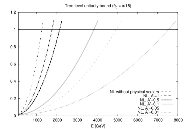
Figure 4: Tree-level unitarity bound. The intersection between the curves and the horizontal line gives the energy threshold. The black dashed line shows the result for the nonlinearly realized electroweak model without scalar resonances, while the other curves correspond to the nonlinearly realized electroweak model with scalar resonances and various values of the $A^{\prime}$ parameter, namely $A^{\prime}=1$ the black dotted one, $A^{\prime}=0.5$ the black dashed-dotted one, $A^{\prime}=0.1$ the grey solid one, $A^{\prime}=0.05$ the grey dashed one and finally $A^{\prime}=0.01$ the grey dotted one.

6 Small $A$ Limit

To a very good approximation one can assume that custodial symmetry holds in the gauge boson sector and thus set $B=0$.

Current LHC data clearly favour a scenario where new physics contributions, resulting in deviations from the SM values, are small [3].

The physically interesting case is therefore achieved in the small $A$ limit. It is interesting to note that the Feynman rules, arising from the expansion of the nonlinear constraint as a power series in $\phi_{a}$’s, cannot be directly used. In fact in the limit $A\rightarrow 0$ one gets

$$\phi_{0}=\sqrt{f^{2}-\phi_{a}^{2}}\sim f\sqrt{1-\frac{\chi^{{}^{\prime}2}_{a}}{A}}\,,$$ (58)

and the power series expansion in terms of $\chi^{{}^{\prime}2}_{a}/A$ cannot be carried out.

In order to overcome this problem the techniques introduced in [29] prove useful. The nonlinear constraint is introduced through a Lagrange multiplier $B$ as follows:

$$S_{constraint}=\int d^{4}x\,B\Big{[}(\sigma+f)^{2}+\phi_{a}^{2}-f^{2}\Big{]}$$ (59)

When the equation of motion for $B$ is imposed, one recovers the solution of the nonlinear constraint

$$\phi_{0}\equiv\sigma+f=\sqrt{f^{2}-\phi_{a}^{2}}$$ (60)

The auxiliary fields $B$ and $\sigma$ are not physical. This is most easily seen by extending the BRST symmetry through the so-called Abelian embedding [29]. The Abelian antighost $\bar{c}$ is transformed into the constraint, while $B$ goes into the Abelian ghost $c$:

$$s\bar{c}=(\sigma+f)^{2}+\phi_{a}^{2}-f^{2}\,,~{}~{}~{}~{}sB=c\,,~{}~{}~{}~{}sc=0\,.$$ (61)

Nilpotency is preserved since the constraint is BRST-invariant. Then one can embed the functional $S_{constraint}$ into the following BRST-exact functional:

$$S_{embed}=\int d^{4}x\,s(\bar{c}B)=\int d^{4}x\,\Big{[}B((\sigma+f)^{2}+\phi_{a}^{2}-f^{2})-\bar{c}c\Big{]}$$ (62)

The ghost $c$ is free. Moreover at the asympotic level one gets from eq.(61):

$$\{Q,\bar{c}\}=2f\sigma\,,~{}~{}~{}~{}[Q,\sigma]=0\,,$$

$$[Q,B]=c\,,~{}~{}~{}~{}\{Q,c\}=0\,.$$ (63)

Thus $(\bar{c},\sigma)$ and $(B,c)$ are arranged in BRST doublets, according to their unphysical nature.

The propagators generated by $S_{embed}$ are, in terms of the canonically normalized field $\sigma=\frac{1}{\sqrt{A}}\sigma^{\prime}$:

$$\Delta_{BB}=-i\frac{Ap^{2}}{4f^{2}}\,,~{}~{}~{}\Delta_{B\sigma^{\prime}}=i\frac{\sqrt{A}}{2f}\,,~{}~{}~{}\Delta_{\sigma^{\prime}\sigma^{\prime}}=0\,.$$ (64)

The WPC does not hold in the sector spanned by $\sigma$. This happens since the propagator $\Delta_{B\sigma^{\prime}}$ is a constant and thus one can construct one-loop graphs with a chain of internal $B\sigma^{\prime}$-propagators and an even number of external $\sigma^{\prime}$ legs that have superficial UV degree of divergence $4$, irrespective of the number of external $\sigma^{\prime}$-legs. However, the violation of the WPC is confined to a BRST-exact sector. Indeed, the bleached counterpart of $\sigma^{\prime}$ is precisely the nonlinear constraint

$$\tilde{\sigma}^{\prime}=\frac{\sqrt{A}}{2f^{2}}\Big{[}\sigma^{2}+2f\sigma+\phi_{a}^{2}\Big{]}=\frac{\sqrt{A}}{2f^{2}}s\bar{c}\,.$$ (65)

Therefore $\tilde{\sigma}^{\prime}$ and $\bar{c}$ form a set of coupled BRST doublets and one is guaranteed [30] that they do not contribute to the cohomology of the linearized ST operator. Thus they can appear in the counterterms only through BRST-exact terms.

In order to establish a power-counting in $A$ for the physically relevant amplitudes in the $B=0$, $A\to 0$ limit, we first notice that in the tree-level vertex functional (72) there are no singular terms in the symmetric unprimed basis.

Moreover, the propagators in the primed basis are smooth for $A\rightarrow 0$, as can be seen from eqs.(64) and (80) - (82). As a consequence, singularities for $A\to 0$ can only arise from the interaction terms after the field redefinition to the mass eisgenstates basis (12)

$$\phi_{a}\sim_{A\to 0}\frac{1}{\sqrt{A}}\,\chi^{\prime}_{a}+\dots\,,$$ (66)

where the dots stand for terms which are subleading in the small A limit, and from the replacement $\sigma=\frac{1}{\sqrt{A}}\sigma^{\prime}$ to the canonically normalized $\sigma^{\prime}$ field.

In the gauge boson mass sector, $\sigma$ and $\phi_{a}$ enter at most quadratically in the Stückelberg mass term in eq.(4) at $B=0$ and thus no singular interaction vertices arise.

In the physically relevant sector at zero external sources there are no divergent terms in the gauge-fixing sector. On the other hand, from $S_{embed}$ one gets the following singular interaction vertices:

$$\ \int d^{4}x\,\Big{[}\frac{1}{A}~{}B({\sigma^{\prime}}^{2}+{\chi^{\prime}_{a}}^{2})+\frac{2}{\sqrt{A}}\frac{f}{v}B\chi^{\prime}_{a}\phi^{\prime}_{a}\Big{]}$$ (67)

For instance, the tree-level elastic scattering of physical scalar resonances (charged and CP-odd) is singular in the $A\to 0$ limit. The tree-level graphs for the elastic scattering of charged physical scalar resonances are depicted in Fig. 5. From the previous considerations, it is straightforward to find the behaviour for small $A$ of the contribution of the various graphs to the scattering amplitude. In particular, the contribution coming from the first two graphs does not depend on $A$, the one from graphs 3 and 4 depends on $A$ through the mass of the charged scalar resonance ($\sim M^{4}_{\chi^{\prime}_{\pm}}\sim A^{-2}$), the contribution stemming from graphs 5 and 6 is singular in the small $A$ limit ($\sim A^{-1}$) and moreover it has a bad polynomial behaviour ($\sim s+t$) in the high energy limit, the one from graphs 7 and 8 has the same $A$ behaviour as the squared mass of $\chi^{\prime}_{\pm}$ ($\sim M^{2}_{\chi^{\prime}_{\pm}}\sim A^{-1}$) and finally the contribution coming from graph 9 vanishes when $A\to 0$ ($\sim A^{2}$). This result is consistent with the fact that the physical scalar resonances decouple in the SM limit.

Figure 5: Elastic scattering of charged physical scalar resonances at tree-level

7 Conclusions

A mathematically consistent nonlinearly realized electroweak theory, incorporating physical scalar resonances, has been studied. It fulfills a set of functional identities (LFE, ST identity, b-equations, ghost equations) as well as a natural Hopf algebra selection criterion, embodied in the WPC condition. The LFE controls the deformation of the nonlinearly realized SU(2) gauge symmetry, induced by radiative corrections, order by order in the loop expansion. Stability of the gauge-fixing is encoded in the b-equations and the ghost equations. In the nonlinearly realized theory the Weinberg relation between the mass of the $Z$ and the $W$ bosons is not automatically fulfilled and, as a consequence, two independent mass invariants exist. The procedure to implement the ’t Hooft gauge in the presence of two mass invariants, while respecting the defining functional identities and the WPC, has been given. The ST identity in turn guarantees the fulfillment of physical unitarity (i.e. cancellation of intermediate ghost states in physical amplitudes).

The model interpolates between the Higgs and a purely Stückelberg scenario. It is impossible to accommodate a single physical scalar resonance without violating the WPC. The theory therefore makes definite predictions on the BSM sector: there must be four scalar resonances, two charged ones and two neutral ones, one CP-even (to be eventually identified with the $125~{}GeV$ resonance recently discovered at LHC) and one CP-odd.

We have found that if even a small fraction of the mass is generated by the Stückelberg mechanism, the Froissart bound for the scattering of longitudinally polarized $W$ bosons is violated at sufficiently high energies already at tree-level, despite the exchange of a physical scalar resonance. This feature is a characteristic footprint of nonlinearly realized theories.

An important issue is whether one can already exclude from the present LHC7-8 data the presence of a Stückelberg component in the electroweak SSB mechanism realized in Nature. As a necessary preliminary step in this direction, we have analyzed the formal properties of the model in the $B=0$ (the $\rm SU(2)_{R}$ custodial symmetry holds in the gauge boson sector), small $A$ limit, which is believed to be in a first approximation the physically relevant scenario, since BSM effects, if present, have to be small.

In this limit the Feynman rules obtained by expanding the solution of the SU(2) nonlinear constraint in powers of the coordinates $\phi_{a}$ of the SU(2) group element cannot be used. In order to overcome this problem, an approach based on the introduction of a Lagrange multiplier in the so-called Abelian embedding formalism has been studied. The WPC is violated, but only in an unphysical BRST-exact sector of the theory. We have also derived a power-counting to identify the leading diagrams in the small $A$ limit. This is a necessary tool for the forthcoming phenomenological analysis of the model.

Appendix A Conventions

The SU(2) and ${\rm U(1)_{Y}}$ gauge fields are $A_{a\mu}$ and $B_{\mu}$ respectively. The charged $W$, the $Z$ and photon $A$ fields are given by

$$W^{\pm}_{\mu}=\frac{1}{\sqrt{2}}(A^{1}_{\mu}\mp iA^{2}_{\mu})\,,~{}~{}~{}Z_{\mu}=c_{W}A^{3}_{\mu}+s_{W}B_{\mu}\,,~{}~{}~{}A_{\mu}=-s_{W}A^{3}_{\mu}+c_{W}B_{\mu}\,.$$ (68)

In the above equation $c_{W}$ and $s_{W}$ are the cosine and the sine of the Weinberg angle:

$$c_{W}=\frac{g}{G}\,,~{}~{}~{}~{}s_{W}=\frac{g^{\prime}}{G}\,,~{}~{}~{}~{}G=\sqrt{g^{2}+{g^{\prime}}^{2}}\,.$$ (69)

$g,g^{\prime}$ are the SU(2) and the hypercharge ${\rm U(1)_{Y}}$ coupling constants respectively. The covariant derivative of the matrix $\chi=(v+X_{0})+i\chi_{a}\tau_{a}$ is

$$D_{\mu}\chi=\partial_{\mu}\chi-igA^{a}_{\mu}\frac{\tau^{a}}{2}\chi-ig^{\prime}B_{\mu}\chi\frac{\tau_{3}}{2}$$ (70)

and similarly for $\Omega$.

Appendix B BRST Transformations

$c_{a}$ are the SU(2) ghosts, $c_{0}$ is the hypercharge ${\rm U(1)_{Y}}$ ghost. The BRST transformations are

$$sA_{a\mu}=\partial_{\mu}c_{a}+g\epsilon_{abc}A_{b\mu}c_{c}\,,\qquad sB_{\mu}=\partial_{\mu}c_{0}\,,\qquad sc_{a}=-\frac{1}{2}\epsilon_{abc}c_{b}c_{c}\,,$$

$$s\chi=igc_{a}\frac{\tau_{a}}{2}\chi+ig^{\prime}\chi c_{0}\frac{\tau_{3}}{2},\qquad s\Omega=igc_{a}\frac{\tau_{a}}{2}\Omega+ig^{\prime}\Omega c_{0}\frac{\tau_{3}}{2}\,,$$

$$sL=igc_{a}\frac{\tau_{a}}{2}L+\frac{i}{2}g^{\prime}c_{0}Y_{L}L\,,\qquad sR=\frac{i}{2}g^{\prime}c_{0}(Y_{L}+\tau_{3})R\,,$$

$$s\bar{c}_{a}=b_{a}\,,\qquad sb_{a}=0\,,\qquad s\bar{c}_{0}=b_{0}\,,\qquad sb_{0}=0\,$$

$$s\phi_{0}^{*}=-K_{0}\,,~{}~{}~{}sK_{0}=0\,,~{}~{}~{}sV_{a\mu}=\Omega_{a\mu}\,,~{}~{}~{}s\Omega_{a\mu}=0\,,~{}~{}~{}s\hat{\Omega}=\Theta\,,~{}~{}~{}s\Theta=0\,.$$ (71)

$Y_{L}$ is the hypercharge of the doublet $L$.

The BRST transformation of the background fields $V_{a\mu}$, $\hat{\Omega}$ guarantee that the physical observables of the theory are not modified [31], since the cohomology of the BRST differential is unchanged by the inclusion of the background fields as BRST doublets [30],[32]. This implies that the dependence on the background is generated via a canonical transformation respecting the ST identity [33].

Appendix C Tree-level Vertex Functional

The tree-level action of the nonlinearly realized theory is

$$\Gamma^{(0)} = \int d^{4}x\,\Big{(}-\frac{1}{4}G_{a\mu\nu}G_{a}^{\mu\nu}-\frac{1}{4}F_{\mu\nu}^{2}+\frac{1}{4}~{}{\rm Tr}(D_{\mu}\chi)^{\dagger}D^{\mu}\chi$$ (72)

$$\qquad\qquad\frac{Af^{2}}{4}~{}{\rm Tr}(D_{\mu}\Omega)^{\dagger}D^{\mu}\Omega+\frac{Bf^{4}}{16}~{}[{\rm Tr}(\Omega^{\dagger}D_{\mu}\Omega\tau_{3})]^{2}$$

$$\qquad\qquad-\frac{\lambda}{16}\Big{[}{\rm Tr}(\chi^{\dagger}\chi)\Big{]}^{2}+\frac{\mu^{2}}{2}{\rm Tr}(\chi^{\dagger}\chi)-\frac{1}{2}M_{3}^{2}\tilde{\chi}_{3}^{2}-M^{2}_{\pm}\tilde{\chi}^{+}\tilde{\chi}^{-}$$

$$\qquad\qquad+\sum_{L}\bar{L}(i\partial\!\!\!/+gA\!\!\!/-\frac{g^{\prime}}{2}Y_{L}B\!\!\!\!/)L+\sum_{R}\bar{R}(i\partial\!\!\!/-\frac{g^{\prime}}{2}(Y_{L}+\tau_{3})B\!\!\!\!/)R$$

$$\qquad\qquad+\sum_{i,j}\Big{[}\bar{L}^{l}_{i}Y^{l}_{ij}l^{d}_{Rj}\Xi+\bar{L}^{q}_{i}Y^{d}_{ij}q^{d}_{Rj}\Xi+\bar{L}^{q}_{i}Y^{u}_{ij}q^{u}_{Rj}\Xi^{C}+h.c.\Big{]}$$

$$\qquad\qquad+\sum_{i,j,k}\Big{[}\bar{\tilde{l}}^{d}_{Li}m^{l}_{ik}y^{l}_{kj}l^{d}_{Rj}+\bar{\tilde{q}}^{u}_{Li}m^{u}_{ik}y^{u}_{kj}q^{u}_{Rj}+\bar{\tilde{q}}^{d}_{Li}m^{d}_{ik}y^{d}_{kj}q^{d}_{Rj}+h.c.\Big{]}$$

$$\qquad\qquad+\frac{1}{4\xi}b_{a}^{2}+b_{a}{\cal F}_{a}-\bar{c}_{a}s{\cal F}_{a}+\frac{1}{4\xi}b_{0}^{2}+b_{0}{\cal F}_{0}-\bar{c}_{0}s{\cal F}_{0}$$

$$\qquad\qquad+A^{*}_{a\mu}sA_{a\mu}+c^{*}_{a}sc_{a}+\chi_{0}^{*}s\chi_{0}+\chi_{a}^{*}s\chi_{a}+\phi_{a}^{*}s\phi_{a}+K_{0}\phi_{0}+\phi_{0}^{*}s\phi_{0}$$

$$\qquad\qquad+\sum_{L}\Big{[}L^{*}sL+\bar{L}^{*}s\bar{L}\Big{]}+\sum_{R}\Big{[}R^{*}sR+\bar{R}^{*}s\bar{R}\Big{]}\Big{)}\,.$$

In the above equation we have used the following notation for the fermions. $L$ ranges over the set of left SU(2) doublets

$$L\in\Big{\{}\begin{pmatrix}l^{u}_{Lj}\\ l^{d}_{Lj}\end{pmatrix}\,,\begin{pmatrix}q^{u}_{Lj}\\ q^{d}_{Lj}\end{pmatrix}\,,~{}~{}~{}~{}j=1,2,3\Big{\}}$$ (73)

The lepton doublet of the generation $i$ is denoted by $L^{l}_{i}=\begin{pmatrix}l^{u}_{Li}\\ l^{d}_{Li}\end{pmatrix}$, the quark doublet by $L^{q}_{i}=\begin{pmatrix}q^{u}_{Li}\\ q^{d}_{Li}\end{pmatrix}$. Color indices are suppressed. $\tilde{l}^{u(d)}_{Li}$ and $\tilde{q}^{u(d)}_{Li}$ are the components of the bleached doublets

$$\tilde{L}^{l}_{i}=\Omega^{\dagger}L^{l}_{i}=\begin{pmatrix}{\tilde{l}}^{u}_{Li}\\ {\tilde{l}}^{d}_{Li}\end{pmatrix}\,,\qquad\qquad\tilde{L}^{q}_{i}=\Omega^{\dagger}L^{q}_{i}=\begin{pmatrix}{\tilde{q}}^{u}_{Li}\\ {\tilde{q}}^{d}_{Li}\end{pmatrix}\,.$$ (74)

The matrices $m^{l(u,d)}$ are taken to be diagonal, $m^{l(u,d)}_{ik}=m^{l(u,d)}_{i}\delta_{ik}$ (no sum over $i$).

The right components are also formally arranged in doublets

$$R\in\Big{\{}\begin{pmatrix}l^{u}_{Rj}\\ l^{d}_{Rj}\end{pmatrix}\,,\begin{pmatrix}q^{u}_{Rj}\\ q^{d}_{Rj}\end{pmatrix}\,,~{}~{}~{}~{}j=1,2,3\Big{\}}$$ (75)

The matrix $\chi$ is decomposed as

$$\chi_{\alpha\beta}=\Xi^{C}_{\alpha}\Xi_{\beta}\,,~{}~{}~{}~{}\Xi=\begin{pmatrix}i\chi_{1}+\chi_{2}\\ \chi_{0}-i\chi_{3}\end{pmatrix}\,,~{}~{}~{}\Xi^{C}=i\tau_{2}\Xi^{*}=\begin{pmatrix}\chi_{0}+i\chi_{3}\\ i\chi_{1}-\chi_{2}\end{pmatrix}\,.$$ (76)

$Y^{l(u,d)}$ are external sources. They are required to have maximal UV degree $1$. In this way the structure of the Yukawa couplings in eq.(72) is automatically enforced and consequently tree-level scalar boson mediated flavour changing neutral currents are suppressed [9]. Yukawa interactions and fermion masses are induced by the shift $Y^{l(u,d)}\rightarrow y^{l(u,d)}+Y^{l(u,d)}$. After diagonalization of $y^{l(u,d)}$, the masses of the fermions become

$$m_{i}^{l(u,d)^{\prime}}=(m^{l(u,d)}_{i}+v)y^{l(u,d)}_{i}\,.$$ (77)

The term proportional to $v$ is the same as in the SM. The parameters $m^{l(u,d)}_{i}$ are not fixed by symmetry requirements or the WPC. They arise since the gauge symmetry is nonlinearly realized and therefore the bleaching procedure can be used to add independent fermion mass invariants. $m^{l(u,d)}_{i}$ are expected to be small: in the limit $B=0$, small $A$, one may take $m^{l(u,d)}_{i}\sim\sqrt{A}v$. With this choice no divergent vertices arise in the fermionic sector in the limit $A\rightarrow 0$.

Appendix D ’t Hooft Gauge-fixing in the Nonlinearly Realized Theory

We summarize here the propagators in the ’t Hooft gauge. The gauge-fixing functions in eqs.(32) and (33) read in components

$${\cal F}_{a} = \partial A_{a}-\partial V_{a}+g\epsilon_{abc}V_{b\mu}A^{\mu}_{c}$$

$$+\frac{M_{W}}{4\xi f}\frac{1}{\sqrt{1+\frac{f^{2}}{v^{2}}\,C_{b}}}\Big{[}\delta_{ab}(\hat{\phi}_{0}^{2}-\hat{\phi}_{c}^{2})\Big{(}\frac{f}{v}C_{b}\tilde{q}_{b}+\tilde{r}_{b}\Big{)}+2\hat{\phi}_{a}\hat{\phi}_{b}\Big{(}\frac{f}{v}C_{b}\tilde{q}_{b}+\tilde{r}_{b}\Big{)}$$

$$\qquad\qquad\qquad+2\epsilon_{abc}\hat{\phi}_{0}\Big{(}\frac{f}{v}C_{b}\tilde{q}_{b}+\tilde{r}_{b}\Big{)}\hat{\phi}_{c}\Big{]}\,,$$

$${\cal F}_{0} = \partial B+\frac{g^{\prime}}{g}\frac{M_{W}}{2f\xi}(1+\kappa)\frac{1}{\sqrt{1+\frac{f^{2}}{v^{2}}C_{3}}}\Big{[}\hat{\phi}_{0}\Big{(}\frac{f}{v}C_{3}\phi_{3}+\chi_{3}\Big{)}-\hat{\phi}_{3}\Big{(}\frac{f}{v}C_{3}\phi_{0}+\chi_{0}\Big{)}$$ (78)

$$\qquad\qquad\qquad+\epsilon_{3bc}\hat{\phi}_{b}\Big{(}\frac{f}{v}C_{3}\phi_{c}+\chi_{c}\Big{)}\Big{]}\,.$$

To diagonalize the quadratic part of the tree-level vertex functional at zero background fields we perform the following transformation:

$$b^{\prime}_{a}=b_{a}+2\xi\Big{(}\partial A_{a}+\frac{M_{W}}{2\xi}e_{a}\phi^{\prime}_{a}\Big{)}\,,~{}~{}~{}~{}~{}b^{\prime}_{0}=b_{0}+2\xi\Big{[}\partial B+\frac{g^{\prime}}{g}\frac{M_{W}}{2\xi}(1+\kappa)\phi^{\prime}_{3}\Big{]}\,.$$ (79)

We give here the propagators in the symmetric basis, which is most useful in establishing the WPC:

$$\Delta_{A_{1\mu}A_{1\nu}}=\Delta_{A_{2\mu}A_{2\nu}}=\frac{i}{-p^{2}+M_{W}^{2}}T_{\mu\nu}+\frac{i}{-2\xi p^{2}+M_{W}^{2}}L_{\mu\nu}\,,$$

$$\Delta_{A_{1\mu}A_{2\nu}}=\Delta_{A_{1\mu}A_{3\nu}}=\Delta_{A_{2\mu}A_{3\nu}}=0\,,$$

$$\Delta_{A_{3\mu}A_{3\nu}}=iT_{\mu\nu}\Big{(}\frac{s_{W}^{2}}{-p^{2}}+\frac{c_{W}^{2}}{-p^{2}+M_{Z}^{2}}\Big{)}+iL_{\mu\nu}\Big{(}\frac{s_{W}^{2}}{2\xi p^{2}}+\frac{c_{W}^{2}}{-2\xi p^{2}+M_{Z}^{2}}\Big{)}\,,$$

$$\Delta_{A_{3\mu}B_{\nu}}=-ic_{W}s_{W}T_{\mu\nu}\Big{(}-\frac{1}{p^{2}}-\frac{1}{-p^{2}+M_{Z}^{2}}\Big{)}-ic_{W}s_{W}L_{\mu\nu}\Big{(}\frac{1}{2\xi p^{2}}-\frac{1}{-2\xi p^{2}+M_{Z}^{2}}\Big{)}\,,$$

$$\Delta_{B_{\mu}B_{\nu}}=iT_{\mu\nu}\Big{(}\frac{c_{W}^{2}}{-p^{2}}+\frac{s_{W}^{2}}{-p^{2}+M_{Z}^{2}}\Big{)}+iL_{\mu\nu}\Big{(}\frac{c_{W}^{2}}{2\xi p^{2}}+\frac{s_{W}^{2}}{-2\xi p^{2}+M_{Z}^{2}}\Big{)}\,,$$

$$\Delta_{A_{1\mu}B_{\nu}}=\Delta_{A_{2\mu}B_{\nu}}=0\,,~{}~{}~{}~{}~{}\Delta_{\phi^{\prime}_{i}\phi^{\prime}_{j}}=\delta_{ij}\frac{i}{p^{2}-\frac{M_{W}^{2}}{2\xi}}\,,~{}~{}~{}i,j=1,2\,,~{}~{}~{}~{}\Delta_{\phi^{\prime}_{3}\phi^{\prime}_{3}}=\frac{i}{p^{2}-\frac{M_{Z}^{2}}{2\xi}}\,,$$

$$\Delta_{b^{\prime}_{a}b^{\prime}_{b}}=2i\xi\delta_{ab}\,,~{}~{}~{}~{}a,b=1,2,3\,,~{}~{}~{}~{}\Delta_{b^{\prime}_{0}b^{\prime}_{0}}=2i\xi\,,$$

$$\Delta_{\bar{c}_{i}c_{j}}=\delta_{ij}\frac{i}{p^{2}-\frac{M_{W}^{2}}{2\xi}}\,,~{}~{}~{}~{}i,j=1,2\,,~{}~{}~{}~{}\Delta_{\bar{c}_{3}c_{3}}=\frac{i}{p^{2}-\frac{M_{Z}^{2}}{2\xi}}\,,~{}~{}~{}\Delta_{\bar{c}_{0}c_{0}}=\frac{i}{p^{2}}\,.$$ (80)

The mixed $A-\phi$ propagators are zero. Fermion propagators are the usual ones

$$\Delta_{\bar{f}f}=\frac{i}{p\!\!\!/-m^{\prime}_{f}}$$ (81)

while for the $\chi^{\prime}_{a}$

$$\Delta_{\chi^{\prime}_{i}\chi^{\prime}_{j}}=\delta_{ij}\frac{i}{p^{2}-M^{2}_{\chi^{\prime}_{\pm}}}\,,~{}~{}i,j=1,2,~{}~{}~{}\Delta_{\chi^{\prime}_{3}\chi^{\prime}_{3}}=\frac{i}{p^{2}-M^{2}_{\chi^{\prime}_{3}}}\,,~{}~{}~{}\Delta_{X_{0}X_{0}}=\frac{i}{p^{2}-M^{2}_{X_{0}}}\,.$$ (82)

Appendix E Functional Identities

We collect here in compact form the functional identities of the theory:

• the b-equations

  $$\frac{\delta\Gamma}{\delta b_{a}}=\frac{1}{2\xi}b_{a}+\left.{\cal F}_{a}\right|_{\phi_{0}\rightarrow\frac{\delta\Gamma}{\delta K_{0}}}\,,$$

  $$\frac{\delta\Gamma}{\delta b_{0}}=\frac{1}{2\xi}b_{0}+\left.{\cal F}_{0}\right|_{\phi_{0}\rightarrow\frac{\delta\Gamma}{\delta K_{0}}}\,.$$ (83)

  Notice that the r.h.s. of the above equations is linear in the quantum fields. The nonlinear constraint $\phi_{0}$ is generated by taking a derivative w.r.t. the external source $K_{0}$.

• the ghost equations

  $$\frac{\delta\Gamma}{\delta{\bar{c}}_{a}} = -D^{\mu}[V]_{ab}\frac{\delta\Gamma}{\delta A^{*b}_{\mu}}+D_{\mu}[A]_{ab}\Omega^{\mu}_{b}$$

  $$-\frac{M_{W}}{4\xi f}\frac{1}{\sqrt{1+\frac{f^{2}}{v^{2}}C_{b}}}\Big{\{}\frac{f}{v}C_{b}{\rm Tr}\Big{[}\hat{\Omega}\Big{(}\hat{\phi}_{0}\frac{\delta\Gamma}{\delta\phi_{b}^{*}}-\hat{\phi}_{b}\frac{\delta\Gamma}{\delta\phi_{0}^{*}}-\epsilon_{bdc}\frac{\delta\Gamma}{\delta\phi^{*}_{d}}\hat{\phi}_{c}\Big{)}e_{b}\tau_{b}\hat{\Omega}^{\dagger}\tau_{a}\Big{]}$$

  $$\qquad\qquad\qquad\quad~{}~{}~{}~{}~{}~{}+{\rm Tr}\Big{[}\hat{\Omega}\Big{(}\hat{\phi}_{0}\frac{\delta\Gamma}{\delta\chi_{b}^{*}}-\hat{\phi}_{b}\frac{\delta\Gamma}{\delta\chi_{0}^{*}}-\epsilon_{bdc}\frac{\delta\Gamma}{\delta\chi^{*}_{d}}\hat{\phi}_{c}\Big{)}e_{b}\tau_{b}\hat{\Omega}^{\dagger}\tau_{a}\Big{]}$$

  $$\qquad\qquad\qquad\quad~{}+\frac{f}{v}C_{b}{\rm Tr}\Big{[}\hat{\Omega}\Big{(}\Theta_{0}\phi_{b}-\Theta_{b}\frac{\delta\Gamma}{\delta K_{0}}-\epsilon_{bdc}\phi_{d}\Theta_{c}\Big{)}e_{b}\tau_{b}\hat{\Omega}^{\dagger}\tau_{a}\Big{]}$$

  $$\qquad\qquad\qquad\quad~{}~{}~{}~{}~{}~{}+{\rm Tr}\Big{[}\hat{\Omega}\Big{(}\Theta_{0}\chi_{b}-\Theta_{b}\chi_{0}-\epsilon_{bdc}\chi_{d}\Theta_{c}\Big{)}e_{b}\tau_{b}\hat{\Omega}^{\dagger}\tau_{a}\Big{]}\Big{\}}$$

  $$-\frac{fM_{W}}{4\xi\sqrt{1+\frac{f^{2}}{v^{2}}C_{b}}}\Big{\{}\frac{f}{v}C_{b}{\rm Tr}\Big{[}\Theta~{}\tilde{q}_{b}\frac{\tau_{b}}{2}~{}\widehat{\Omega}^{\dagger}\tau_{a}+\widehat{\Omega}~{}\tilde{q}_{b}\frac{\tau_{b}}{2}~{}\Theta^{\dagger}\tau_{a}\Big{]}$$

  $$\qquad\qquad\qquad~{}~{}~{}~{}~{}~{}~{}+{\rm Tr}\Big{[}\Theta~{}\tilde{r}_{b}\frac{\tau_{b}}{2}~{}\widehat{\Omega}^{\dagger}\tau_{a}+\widehat{\Omega}~{}\tilde{r}_{b}\frac{\tau_{b}}{2}~{}\Theta^{\dagger}\tau_{a}\Big{]}\Big{\}}\,,$$

  $$\frac{\delta\Gamma}{\delta{\bar{c}}_{0}} = -\square c_{0}-\frac{g^{\prime}}{g}\frac{M_{W}}{2f\xi}\frac{1+\kappa}{\sqrt{1+\frac{f^{2}}{v^{2}}C_{3}}}\times$$ (84)

  $$\qquad\Big{[}\frac{f}{v}C_{3}\Big{(}\hat{\phi}_{0}\frac{\delta\Gamma}{\delta\phi_{3}^{*}}-\hat{\phi}_{3}\frac{\delta\Gamma}{\delta\phi_{0}^{*}}-\epsilon_{3dc}\frac{\delta\Gamma}{\delta\phi^{*}_{d}}\hat{\phi}_{c}\Big{)}+\frac{f}{v}C_{3}\Big{(}\Theta_{0}\phi_{3}-\Theta_{3}\frac{\delta\Gamma}{\delta K_{0}}-\epsilon_{3dc}\phi_{d}\Theta_{c}\Big{)}$$

  $$\qquad~{}~{}~{}+\hat{\phi}_{0}\frac{\delta\Gamma}{\delta\chi_{3}^{*}}-\hat{\phi}_{3}\frac{\delta\Gamma}{\delta\chi_{0}^{*}}-\epsilon_{3dc}\frac{\delta\Gamma}{\delta\chi^{*}_{d}}\hat{\phi}_{c}+\Theta_{0}\chi_{3}-\Theta_{3}\chi_{0}-\epsilon_{3dc}\chi_{d}\Theta_{c}\Big{]}\,.$$

• the Local Functional Equation

  $$\!\!\!\!\!\!\!\!\!({\cal W}\Gamma)_{a} \equiv -\partial_{\mu}\frac{\delta\Gamma}{\delta V_{a\mu}}+g\epsilon_{abc}V_{c\mu}\frac{\delta\Gamma}{\delta V_{b\mu}}-\partial_{\mu}\frac{\delta\Gamma}{\delta A_{a\mu}}+g\epsilon_{abc}A_{c\mu}\frac{\delta\Gamma}{\delta A_{b\mu}}$$ (85)

  $$+\frac{g}{2}K_{0}\phi_{a}+\frac{g}{2}\frac{\delta\Gamma}{\delta K_{0}}\frac{\delta\Gamma}{\delta\phi_{a}}+\frac{g}{2}\epsilon_{abc}\phi_{c}\frac{\delta\Gamma}{\delta\phi_{b}}+\frac{g}{2}\chi_{0}\frac{\delta\Gamma}{\delta\chi_{a}}+\frac{g}{2}\epsilon_{abc}\chi_{c}\frac{\delta\Gamma}{\delta\chi_{b}}$$

  $$+g\epsilon_{abc}b_{c}\frac{\delta\Gamma}{\delta b_{b}}+g\epsilon_{abc}\bar{c}_{c}\frac{\delta\Gamma}{\delta\bar{c}_{b}}+g\epsilon_{abc}c_{c}\frac{\delta\Gamma}{\delta c_{b}}$$

  $${+\frac{i}{2}g\tau_{a}L\frac{\delta\Gamma}{\delta L}-\frac{i}{2}g\bar{L}\tau_{a}\frac{\delta\Gamma}{\delta\bar{L}}-\frac{i}{2}gL^{*}\tau_{a}\frac{\delta\Gamma}{\delta L^{*}}+\frac{i}{2}g\tau_{a}\bar{L}^{*}\frac{\delta\Gamma}{\delta\bar{L}^{*}}}$$

  $$+g\epsilon_{abc}\Theta_{c\mu}\frac{\delta\Gamma}{\delta\Theta_{b\mu}}+g\epsilon_{abc}A^{*}_{c\mu}\frac{\delta\Gamma}{\delta A^{*}_{b\mu}}+g\epsilon_{abc}c^{*}_{c}\frac{\delta\Gamma}{\delta c^{*}_{b}}$$

  $$-\frac{g}{2}\phi_{0}^{*}\frac{\delta\Gamma}{\delta\phi^{*}_{a}}+\frac{g}{2}\epsilon_{abc}\phi^{*}_{c}\frac{\delta\Gamma}{\delta\phi^{*}_{b}}+\frac{g}{2}\phi_{a}^{*}\frac{\delta\Gamma}{\delta\phi_{0}^{*}}-\frac{g}{2}\chi_{0}^{*}\frac{\delta\Gamma}{\delta\chi^{*}_{a}}+\frac{g}{2}\epsilon_{abc}\chi^{*}_{c}\frac{\delta\Gamma}{\delta\chi^{*}_{b}}+\frac{g}{2}\chi_{a}^{*}\frac{\delta\Gamma}{\delta\chi_{0}^{*}}$$

  $$-\frac{g}{2}\Theta_{0}\frac{\delta\Gamma}{\delta\Theta_{a}}+\frac{g}{2}\epsilon_{abc}\Theta_{c}\frac{\delta\Gamma}{\delta\Theta_{b}}+\frac{g}{2}\Theta_{a}\frac{\delta\Gamma}{\delta\Theta_{0}}=0\,.$$

• the Slavnov-Taylor identity

  $${\cal S}(\Gamma) = \int d^{4}x\,\Big{(}\frac{\delta\Gamma}{\delta A^{*}_{a\mu}}\frac{\delta\Gamma}{\delta A^{a}_{\mu}}+\frac{\delta\Gamma}{\delta\chi^{*}_{a}}\frac{\delta\Gamma}{\delta\chi_{a}}+\frac{\delta\Gamma}{\delta\chi^{*}_{0}}\frac{\delta\Gamma}{\delta\chi_{0}}+\frac{\delta\Gamma}{\delta F^{*}}\frac{\delta\Gamma}{\delta F}+\frac{\delta\Gamma}{\delta\bar{F}^{*}}\frac{\delta\Gamma}{\delta\bar{F}}$$ (86)

  $$\qquad\qquad+\partial_{\mu}c_{0}\frac{\delta\Gamma}{\delta B_{\mu}}+\frac{\delta\Gamma}{\delta c_{a}^{*}}\frac{\delta\Gamma}{\delta c_{a}}+\frac{\delta\Gamma}{\delta\phi_{a}^{*}}\frac{\delta\Gamma}{\delta\phi_{a}}+b_{a}\frac{\delta\Gamma}{\delta\bar{c}_{a}}+b_{0}\frac{\delta\Gamma}{\delta\bar{c}_{0}}$$

  $$\qquad\qquad-K_{0}\frac{\delta\Gamma}{\delta\phi_{0}^{*}}+\Omega_{a\mu}\frac{\delta\Gamma}{\delta V_{a\mu}}+\Theta_{0}\frac{\delta\Gamma}{\delta\hat{\phi}_{0}}+\Theta_{a}\frac{\delta\Gamma}{\delta\hat{\phi}_{a}}\Big{)}=0$$

  where $F$ runs over $L,R$.

References

• [1] G. Aad et al. [ATLAS Collaboration], Phys. Lett. B 716 (2012) 1 [arXiv:1207.7214 [hep-ex]].
• [2] S. Chatrchyan et al. [CMS Collaboration], Phys. Lett. B 716 (2012) 30 [arXiv:1207.7235 [hep-ex]].
• [3] P. P. Giardino, K. Kannike, I. Masina, M. Raidal and A. Strumia, “The universal Higgs fit,” arXiv:1303.3570 [hep-ph].
• [4] J. Ellis and T. You, “Updated Global Analysis of Higgs Couplings,” arXiv:1303.3879 [hep-ph].
• [5] E. C. G. Stueckelberg, Helv. Phys. Acta 11 (1938) 299.
• [6] H. Ruegg and M. Ruiz-Altaba, Int. J. Mod. Phys. A 19 (2004) 3265 [hep-th/0304245].
• [7] R. Contino, M. Ghezzi, C. Grojean, M. Muhlleitner and M. Spira, “Effective Lagrangian for a light Higgs-like scalar,” arXiv:1303.3876 [hep-ph].
• [8] C. N. Leung, S. T. Love and S. Rao, Z. Phys. C 31 (1986) 433; W. Buchmuller and D. Wyler, Nucl. Phys. B 268 (1986) 621; B. Grzadkowski, M. Iskrzynski, M. Misiak and J. Rosiek, JHEP 1010 (2010) 085 [arXiv:1008.4884 [hep-ph]].
• [9] D. Binosi and A. Quadri, JHEP 1302 (2013) 020 [arXiv:1210.2637 [hep-ph]].
• [10] J. Gomis and S. Weinberg, Nucl. Phys. B 469 (1996) 473 [hep-th/9510087].
• [11] R. Ferrari, JHEP 0508 (2005) 048 [hep-th/0504023].
• [12] R. Ferrari and A. Quadri, JHEP 0601 (2006) 003 [hep-th/0511032].
• [13] R. Ferrari and A. Quadri, Int. J. Theor. Phys.  45 (2006) 2497 [hep-th/0506220].
• [14] A. Quadri, Eur. Phys. J. C 70 (2010) 479 [arXiv:1007.4078 [hep-th]].
• [15] K. Ebrahimi-Fard and F. Patras, Annales Henri Poincare 11 (2010) 943 [arXiv:1003.1679 [math-ph]].
• [16] A. Connes and D. Kreimer, Commun. Math. Phys.  216 (2001) 215 [hep-th/0003188].
• [17] A. Connes and D. Kreimer, Commun. Math. Phys.  210 (2000) 249 [hep-th/9912092].
• [18] D. Bettinelli, R. Ferrari and A. Quadri, Phys. Rev. D 77 (2008) 045021 [arXiv:0705.2339 [hep-th]].
• [19] D. Bettinelli, R. Ferrari and A. Quadri, Acta Phys. Polon. B 41 (2010) 597 [Erratum-ibid. B 43 (2012) 483] [arXiv:0809.1994 [hep-th]].
• [20] D. Bettinelli, D. Binosi, A. Quadri, in preparation.
• [21] M. Froissart, Phys. Rev.  123 (1961) 1053.
• [22] R. Ferrari and A. Quadri, JHEP 0411 (2004) 019 [hep-th/0408168].
• [23] D. Bettinelli, R. Ferrari and A. Quadri, Phys. Rev. D 77 (2008) 105012 [Erratum-ibid. D 85 (2012) 129901] [arXiv:0709.0644 [hep-th]].
• [24] D. Bettinelli, R. Ferrari and A. Quadri, Int. J. Mod. Phys. A 24 (2009) 2639 [Erratum-ibid. A 27 (2012) 1292004] [arXiv:0807.3882 [hep-ph]].
• [25] A. Denner, G. Weiglein and S. Dittmaier, Nucl. Phys. B 440 (1995) 95 [hep-ph/9410338]; P. A. Grassi, Nucl. Phys. B 560 (1999) 499 [hep-th/9908188].
• [26] C. Becchi, A. Rouet and R. Stora, Phys. Lett. B 52 (1974) 344; C. Becchi, A. Rouet and R. Stora, Commun. Math. Phys.  42 (1975) 127; C. Becchi, A. Rouet and R. Stora, Annals Phys.  98 (1976) 287.
• [27] B. W. Lee, C. Quigg and H. B. Thacker, Phys. Rev. D 16 (1977) 1519; B. W. Lee, C. Quigg and H. B. Thacker, Phys. Rev. Lett.  38 (1977) 883.
• [28] A. Denner and T. Hahn, Nucl. Phys.  B 525, 27 (1998) [arXiv:hep-ph/9711302].
• [29] A. Quadri, Phys. Rev. D 73 (2006) 065024 [hep-th/0601169].
• [30] A. Quadri, JHEP 0205 (2002) 051 [hep-th/0201122].
• [31] P. A. Grassi, Nucl. Phys. B 462 (1996) 524 [hep-th/9505101]; C. Becchi and R. Collina, Nucl. Phys. B 562 (1999) 412 [hep-th/9907092]; R. Ferrari, M. Picariello and A. Quadri, Annals Phys.  294 (2001) 165 [hep-th/0012090].
• [32] G. Barnich, F. Brandt and M. Henneaux, Phys. Rept.  338 (2000) 439 [hep-th/0002245].
• [33] D. Binosi and A. Quadri, Phys. Rev. D 84 (2011) 065017 [arXiv:1106.3240 [hep-th]]; D. Binosi and A. Quadri, Phys. Rev. D 85 (2012) 121702 [arXiv:1203.6637 [hep-th]].