Is $Z_{c}(3900)$ a molecular state

Abstract

Assuming the newly observed $Z_{c}(3900)$ to be a molecular state of $D\bar{D}^{*}(D^{*}\bar{D})$, we calculate the partial widths of $Z_{c}(3900)\to J/\psi+\pi;\;\psi^{\prime}+\pi;\;\eta_{c}+\rho$ and $D\bar{D}^{*}$ within the light front model (LFM). $Z_{c}(3900)\to J/\psi+\pi$ is the channel by which $Z_{c}(3900)$ was observed, our calculation indicates that it is indeed one of the dominant modes whose width can be in the range of a few MeV depending on the model parameters. Similar to $Z_{b}$ and $Z_{b}^{\prime}$, Voloshin suggested that there should be a resonance $Z_{c}^{\prime}$ at 4030 MeV which can be a molecular state of $D^{*}\bar{D}^{*}$. Then we go on calculating its decay rates to all the aforementioned final states and as well the $D^{*}\bar{D}^{*}$. It is found that if $Z_{c}(3900)$ is a molecular state of ${1\over\sqrt{2}}(D\bar{D}^{*}+D^{*}\bar{D})$, the partial width of $Z_{c}(3900)\to D\bar{D}^{*}$ is rather small, but the rate of $Z_{c}(3900)\to\psi(2s)\pi$ is even larger than $Z_{c}(3900)\to J/\psi\pi$. The implications are discussed and it is indicated that with the luminosity of BES and BELLE, the experiments may finally determine if $Z_{c}(3900)$ is a molecular state or a tetraquark.

I Introduction

Recently the BES collaborationAblikim:2013mio has claimed that a new resonance is observed in the invariance mass spectrum of $J/\psi\pi^{\pm}$ by studying the process $e^{+}e^{-}\to J/\psi\pi^{+}\pi^{-}$ at $\sqrt{s}=4.26$ GeV, which is referred as $Z_{c}(3900)$ with its mass and width being $(3.899\pm 3.6\pm 4.9)$ GeV and $(46\pm 10\pm 10)$ MeV respectively. The BelleLiu:2013dau and CLEOXiao:2013iha also reported the same new structure. Since the resonance is charged it cannot be a charmonium, but its mass and decay modes imply that it has a hidden charm-anticharm structure, therefore it must be an exotic state. In fact, before this discovery, two bottomonium-like charged resonances $Z_{b}(10610)$ and $Z_{b}(10650)$ were observed by BELLEChoi:2003ue and confirmed by BABAR Collaboration:2011gj . Because they cannot be bottomonia, a reasonable postulate is that they are exotic states with constituents of $b\bar{b}u\bar{d}(d\bar{u})$, e.g. they may be molecular states or tetraquarks etc. Observation of similar charged meson $Z_{c}(3900)$ indicates that at the charm energy range there exist similar exotic states. It intrigues enormous interests of theorists Chen:2013coa ; Cui:2013yva ; Zhang:2013aoa ; Wang:2013cya ; Wilbring:2013cha ; Voloshin:2013dpa . For $Z_{c}(3900)$ some authors suggest it to be a molecular stateCui:2013yva ; Zhang:2013aoa ; Wang:2013cya ; Wilbring:2013cha , whereas some others think it as tetraquark or a mixture of the two statesVoloshin:2013dpa . Which one is the true configuration? The answer can only be obtained from experimental measurements. Namely different structures would result in different decay rates for various channels. Therefore, by assuming a special structure, we predict its decay rates for those possible modes, then the theoretical predictions will be tested by further more accurate measurements and their consistency with data would tell us if the postulation about the hadron structure is reasonable. In this paper we will study the strong decays of $Z_{c}(3900)$ which is assumed to be a molecular state with the quantum number $I^{G}(J^{P})=1^{+}(1^{+})$. Assuming $Z_{c}(3900)$ to have constituents of $D\bar{D}^{*}(D^{*}\bar{D})$, we investigate the decays $Z_{c}(3900)\rightarrow J/\psi\pi;\;\psi^{\prime}\pi;\;\eta_{c}\rho$ and $D\bar{D}^{*}$ under this assignment.

Comparing with $Z_{b}(10610)$ and $Z_{b}(10650)$, $Z_{c}(3900)$ has the same light degrees of freedom, so that one may expect another resonance to exist around $4030$ MeV Voloshin:2013dpa and it could be of the molecular structure of $D^{*}\bar{D}^{*}$. With that assignment we calculate the decay rates of $Z_{c}(4030)$ via the aforementioned decay modes for $Z_{c}(3900)$ as well as $D^{*}\bar{D}^{*}$ because this channel is open at the energy 4030 MeV within the same theoretical framework.

In this work, we will extend the light front quark model (LFQM) which was thoroughly studied in literature Jaus ; Ji:1992yf ; Cheng:2004cc ; Cheng:1996if ; Cheng:2003sm ; Choi:2007se ; Hwang:2006cua ; Ke:2007tg ; Ke:2009ed ; Li:2010bb ; Ke:2013zs to investigate the decays of a molecular state. Initially the authorsJaus ; Ji:1992yf constructed the light front quark model (LFQM) which is used to study processes where only mesons are involved. Later Cheng et. al. extended the framework to explore the decays of pentaquarkCheng:2004cc . Along the line we have extended the model to calculate the decay rates of baryons Ke:2007tg . With the LFQM, the theoretical predictions are reasonably consistent with data, it implies that the applications of LFQM to various situations at charm and bottom energy regions are comparatively successful. This success inspires us to extend the light front model to study decays of molecular states.

In this approach the constituents are two mesons instead of a quark and an antiquark in the light front frame. In the covariant case the constituents are not on-shell. The effective interactions between the two concerned constituent mesons are that often adopted when one studies the effects of final state interactionsHaglin:1999xs ; Oh:2000qr ; Lin:1999ad ; Deandrea:2003pv ; Meng:2007cx ; Yuan:2012zw . Namely, by studying such processes, one can extract the effective coupling constants from the data. Since for the molecular states the constituents and interactions are different from the case for quarks, we need to modify the LFQM and then apply the new version to study the exotic hadrons. In this paper we will deduce the form factors for the two-body decays of a molecular state of $I^{G}(J^{P})=1^{+}(1^{+})$, and use them to estimate the decay widths of $Z_{c}(3900)\rightarrow J/\psi\pi;\;\psi^{\prime}\pi;\;\eta_{c}\rho$ and $D\bar{D}^{*}$ by assuming $Z_{c}(3900)$ to be a molecular state of $D\bar{D}^{*}$, then we calculate the rates of $Z_{c}(4030)\rightarrow J/\psi\pi;\;\psi^{\prime}\pi;\;\eta_{c}\rho$ and $D\bar{D}^{*};\;D^{*}\bar{D}^{*}$.

In our calculation, we keep the $q^{+}=0$ condition i.e. $q^{2}<0$ where one of the final mesons ($\pi$ or $D$) is off-shell, thus the obtained form factors are space-like, i.e. unphysical. Then an analytical extension from the space-like region to the time-like region is applied. Letting the meson be on-shell one can get the physical form factor and calculate the corresponding decay widths. The numerical results will offer us information about the structure of $Z_{c}(3900)$ and the possible $Z_{c}(4030)$.

After the introduction we derive the form factor for transitions $Z_{c}(3900)\rightarrow J/\psi\pi;\;\psi^{\prime}\pi;\;\eta_{c}\rho$ and $D\bar{D}^{*}$ and $Z_{c}(4030)\rightarrow J/\psi\pi;\;\psi^{\prime}\pi;\;\eta_{c}\rho$ and $D\bar{D}^{*};\;D^{*}\bar{D}^{*}$ in section II. Then we numerically evaluate the relevant form factors and decay widths in Sec. III, where all input parameters are presented. At last we discuss the implications of the numerical results possibilities, then finally, we draw our conclusion even though it is not very definite so far. Some details About the adopted approach are collected in the appendix.

II the strong decays of $Z_{c}(3900)$ as a $1^{+}$ $D\bar{D}^{*}$ molecular state

In this section we study the strong decays of a $1^{+}$ $D\bar{D}^{*}$ molecular state in the light-front model. In Ref.Jaus ; Ji:1992yf ; Cheng:2003sm the model is used to explore some meson decays. In this paper we extend it to study a molecular state and the interactions between mesons are regarded as effective ones. The configuration of $D\bar{D}^{*}$ molecular state is $\frac{1}{\sqrt{2}}(D\bar{D}^{*}+\bar{D}D^{*})$. By the Feynman diagrams it is also noted that the topological structure for $Z_{c}(3900)\to J/\psi\pi;\;\psi^{\prime}\pi;\;\eta_{c}\rho$ is different from that for $Z_{c}(3900)\to D\bar{D}^{*}$, so we deal with them separately.

II.1 $Z_{c}(3900)\rightarrow J/\psi\pi\,(\rho\eta_{c}\,{\rm or}\,\psi^{\prime}\pi)$

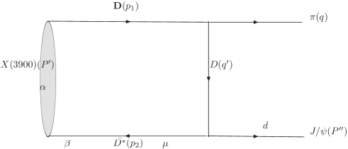
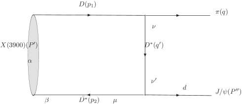
(a)                                (b)

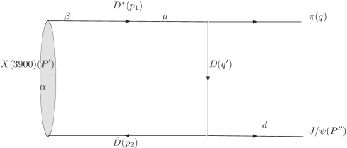
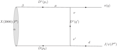
(c)                                (d)

+the Figures exchanged the final states

Figure 1: strong decays of molecular states.

The Feyman diagrams for $Z_{c}(3900)$ decaying into $J/\psi\pi$ by exchanging $D$ or $D^{*}$ mesons are shown in Fig.1. It is noted that when calculate the rates $Z_{c}(3900)\to\rho\eta_{c}$ or $\psi(2s)\pi$, one can simply replace $J/\psi\pi$ by the corresponding final states of $\rho\eta_{c}$ or $\psi(2s)\pi$.

Following the approach in Ref.Cheng:2003sm , the matrix element of diagrams in Fig.1 can be cast as

$${\mathcal{A}}_{11}=i\frac{1}{(2\pi)^{4}}\int d^{4}p_{1}\frac{[H_{A_{01}}(S^{1(a)}_{d\alpha}+S^{1(b)}_{d\alpha})+H_{A_{10}}(S^{1(c)}_{d\alpha}+S^{1(c)}_{d\alpha})]}{N_{1}N_{1}^{\prime}N_{2}}\epsilon_{1}^{d}\epsilon^{\alpha}$$ (1)

with

$$S_{d\alpha}^{1(b)} =\frac{g_{{}_{\psi D^{*}D^{*}}}g_{{}_{\pi DD^{*}}}}{\sqrt{2}}g_{\alpha\beta}g^{\mu\beta}(q_{\nu}+p_{1_{\nu}})g^{\nu\nu^{\prime}}[(q^{\prime}-p_{2})_{d}g_{\mu\nu^{\prime}}-q^{\prime}_{\mu}g_{d\nu^{\prime}}+p_{2\nu^{\prime}}g_{d\mu}]$$

$$\mathcal{F}(m_{1},p_{1})\mathcal{F}(m_{2},p_{2})\mathcal{F}^{2}(m_{D^{*}},q^{\prime}),$$

$$S_{d\alpha}^{1(c)} =\frac{-g_{{}_{\psi DD}}g_{{}_{\pi DD^{*}}}}{\sqrt{2}}g_{\alpha\beta}g^{\mu\beta}(q_{\mu}-q^{\prime}_{\mu})(p_{2d}+q^{\prime}_{d})\mathcal{F}(m_{1},p_{1})\mathcal{F}(m_{2},p_{2})\mathcal{F}^{2}(m_{D},q^{\prime}),$$

$$S_{d\alpha}^{1(d)} =\frac{-g_{{}_{\psi DD^{*}}}g_{{}_{\pi D^{*}D^{*}}}}{\sqrt{2}}g_{\alpha\beta}g^{\mu\beta}g^{\nu\nu^{\prime}}\varepsilon_{a\mu c\nu}p_{1}^{a}q^{\prime c}\varepsilon_{\omega d\nu^{\prime}\rho}P^{\prime\prime\omega}q^{\prime\rho}$$ (2)

$$\mathcal{F}(m_{1},p_{1})\mathcal{F}(m_{2},p_{2})\mathcal{F}^{2}(m_{D^{*}},q^{\prime}),$$

$N_{1}=p_{1}^{2}-m_{1}^{2}+i\varepsilon$, $N_{1}^{\prime}={q^{\prime}}^{2}-m_{q^{\prime}}^{2}+i\varepsilon$ and $N_{2}=p_{2}^{2}-m_{2}^{2}+i\varepsilon$. However $S_{d\alpha}^{1(a)}=0$ since for strong interaction, three pseudoscalars do not couple. The form factor $\mathcal{F}(m_{i},p^{2})=\frac{(m_{i}+\Lambda)^{2}-m_{i}^{2}}{(m_{i}+\Lambda)^{2}-p^{2}}$ compensates the off-shell effect of the intermediate meson ($m_{i}$ and $p$ are the mass and momentum of the intermediate meson ). The vertex function $H_{A}$ will be discussed later. The momentum $p_{i}$ is decomposed as ($p_{i}^{-},p_{i}^{+},{p_{i}}_{\perp}$) in the light-front frame. Integrating out $p_{1}^{-}$ with the methods given in Ref.Cheng:1996if one has

$$\int d^{4}p_{1}\frac{H_{A}S_{d\alpha}}{N_{1}N_{1}^{\prime}N_{2}}{\epsilon_{1}}^{d}{\epsilon}^{\alpha}\rightarrow-i\pi\int dx_{1}d^{2}p_{\perp}\frac{h_{A}\hat{S}_{d\alpha}}{x_{2}\hat{N_{1}}\hat{N_{1}^{\prime}}}{\epsilon_{1}}^{d}{\epsilon}^{\alpha},$$ (3)

with

$$\hat{N}_{1}=x_{1}({M}^{2}-{M_{0}}^{2}),$$

$$\hat{N}_{1}^{{}^{\prime}}=x_{2}q^{2}-x_{1}{M^{\prime}_{0}}^{2}+x_{1}M^{\prime\prime 2}+2p_{\perp}\cdot q_{\perp},$$

$$h_{A}=\sqrt{\frac{x_{1}x_{2}}{m_{1}^{\prime}m_{2}}}(M^{\prime 2}-M_{0}^{\prime 2})h_{A}^{\prime}$$

where $M$ and $M^{\prime}$ represent the masses of initial and finial mesons. The factor $\sqrt{x_{1}x_{2}}(M^{\prime 2}-M_{0}^{\prime 2})$ in the expression of $h_{A}$ was fixed in Ref.Cheng:2003sm and a new factor $\sqrt{\frac{1}{m_{1}m_{2}}}$ appears because the constituents are bosons. $h_{A}^{\prime}$ is defined in the Appendix.

To include the contributions from the zero mode ${p_{1}}_{\mu}$, ${p_{1}}_{\nu}$, ${p_{1}}_{\mu}{p_{1}}_{\nu}$ and $W_{V}$ in $s_{\mu\nu}^{a}$ must be replaced by the appropriate expressions as discussed in Ref.Cheng:2003sm , for example

$$W_{V}\rightarrow w_{V}=M_{0}+m_{1}+m_{2}$$

$${p_{1}}_{\mu}\rightarrow\frac{x_{1}}{2}\mathcal{P}_{\mu}+(\frac{x}{2}-\frac{p_{\perp}\cdot q_{\perp}}{q^{2}})q_{\mu},$$

$$\,\,\,\,\,\,\,\,\,\,\,\,\,\,......$$ (4)

with $\mathcal{P}=P^{\prime}+P^{\prime\prime}$ and $P^{\prime}$ and $P^{\prime\prime}$ are the momenta of the concerned mesons in the initial and final states respectively .

More details about the derivation and some notations such as $M_{0}$ and $\tilde{M}_{0}$ can be found in Ref.Cheng:2003sm . With the replacement, $h_{A}\hat{S}_{d\alpha}$ is decomposed into

$${F_{11}}g_{d\alpha}+{F_{12}}P^{\prime}_{d}P^{\prime\prime}_{\alpha},$$ (5)

with

$${F_{11}}= \frac{g_{{}_{\psi D^{*}D^{*}}}g_{{}_{\pi DD^{*}}}h_{A_{01}}}{2\sqrt{2}}(2\,{A_{1}^{(2)}}-2\,{{m_{1}}}^{2}+{{M^{\prime}}}^{2}+{A_{1}^{(1)}}\,{{M^{\prime}}}^{2}+{A_{2}^{(1)}}\,{{M^{\prime}}}^{2}-{{M^{\prime\prime}}}^{2}+3\,{A_{1}^{(1)}}\,{{M^{\prime\prime}}}^{2}$$

$$-{A_{2}^{(1)}}\,{{M^{\prime\prime}}}^{2}-2\,{\hat{}N_{1}^{\prime}}+{q^{2}}-{A_{1}^{(1)}}\,{q^{2}}-{A_{2}^{(1)}}\,{q^{2}})\mathcal{F}(m_{1},p_{1})\mathcal{F}(m_{2},p_{2})\mathcal{F}^{2}(m_{D^{*}},q^{\prime})+$$

$$-\sqrt{2}g_{{}_{\psi DD}}g_{{}_{\pi DD^{*}}}h_{A_{10}}\,{A_{1}^{(2)}}\mathcal{F}(m_{1},p_{1})\mathcal{F}(m_{2},p_{2})\mathcal{F}^{2}(m_{D},q^{\prime})+$$

$$\frac{g_{{}_{\psi DD^{*}}}g_{{}_{\pi D^{*}D^{*}}}h_{A_{10}}}{2\sqrt{2}}[-2\,{A_{1}^{(2)}}\,({{M^{\prime}}}^{2}-{{M^{\prime\prime}}}^{2}-{q^{2}})+({A_{1}^{(1)}}-{A_{2}^{(2)}}-{A_{3}^{(2)}})\,({{M^{\prime}}}^{4}+{({{M^{\prime\prime}}}^{2}-{q^{2}})}^{2}$$

$$-2\,{{M^{\prime}}}^{2}\,({{M^{\prime\prime}}}^{2}+{q^{2}}))]\mathcal{F}(m_{1},p_{1})\mathcal{F}(m_{2},p_{2})\mathcal{F}^{2}(m_{D^{*}},q^{\prime})$$

$${F_{12}}= \frac{g_{{}_{\psi D^{*}D^{*}}}g_{{}_{\pi DD^{*}}}}{\sqrt{2}}h_{A_{01}}[1-6\,{A_{1}^{(1)}}+{A_{2}^{(2)}}-2\,{A_{3}^{(2)}}-{A_{4}^{(2)}}]\mathcal{F}(m_{1},p_{1})\mathcal{F}(m_{2},p_{2})\mathcal{F}^{2}(m_{D^{*}},q^{\prime})+$$ (6)

$$-\sqrt{2}g_{{}_{\psi DD}}g_{{}_{\pi DD^{*}}}h_{A_{10}}(-2+{A_{1}^{(1)}}+3\,{A_{2}^{(1)}}+{A_{2}^{(2)}}-2\,{A_{3}^{(2)}}-{A_{4}^{(2)}})\mathcal{F}(m_{1},p_{1})\mathcal{F}(m_{2},p_{2})$$

$$\mathcal{F}^{2}(m_{D},q^{\prime})+\frac{g_{{}_{\psi DD^{*}}}g_{{}_{\pi D^{*}D^{*}}}}{\sqrt{2}}h_{A_{10}}[2\,{A_{1}^{(2)}}-({A_{1}^{(1)}}-{A_{2}^{(2)}}-{A_{3}^{(2)}})\,({{M^{\prime}}}^{2}+{{M^{\prime\prime}}}^{2}-{q^{2}})]$$

$$\mathcal{F}(m_{1},p_{1})\mathcal{F}(m_{2},p_{2})\mathcal{F}^{2}(m_{D^{*}},q^{\prime}),$$

where $A_{i}{{}^{(j)}}(i=1\sim 4,j=1\sim 4)$ are determined in Ref.Cheng:2003sm .

We define the form factors as following

$${f_{11}}(m_{1},m_{2})=\frac{1}{32\pi^{3}}\int dx_{2}d^{2}p_{\perp}\frac{F_{11}}{x_{2}\hat{N_{1}}\hat{N_{1}^{\prime}}},$$

$${f_{12}}(m_{1},m_{2})=\frac{1}{32\pi^{3}}\int dx_{2}d^{2}p_{\perp}\frac{F_{12}}{x_{2}\hat{N_{1}}\hat{N_{1}^{\prime}}},$$ (7)

which will be numerically evaluated in next section.

With these form factors the amplitude is obtained as

$${\mathcal{A}}_{11} ={f_{11}}(m_{1},m_{2})\epsilon\cdot\epsilon_{1}+{f_{12}}(m_{1},m_{2}){P^{\prime\prime}\cdot\epsilon P^{\prime}\cdot\epsilon_{1}}.$$ (8)

The amplitude corresponding to the Feynman diagrams which are obtained by exchanging the mesons in the final states of Fig.1 can be formulated by simply exchanging $m_{1}$ and $m_{2}$. The total amplitude is

$$\mathcal{A}_{1} =\mathcal{A}_{11}+\mathcal{A}_{12}$$ (9)

$$=[f_{11}(m_{1},m_{2})+f_{11}(m_{2},m_{1})]\epsilon\cdot\epsilon_{1}+[f_{12}(m_{1},m_{2})+f_{12}(m_{2},m_{1})]{P^{\prime\prime}\cdot\epsilon P^{\prime}\cdot\epsilon_{1}}$$

$$=g_{11}\epsilon\cdot\epsilon_{1}+g_{12}{P^{\prime\prime}\cdot\epsilon P^{\prime}\cdot\epsilon_{1}}.$$

II.2 $Z_{c}(3900)\rightarrow D\bar{D}^{*}$

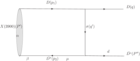
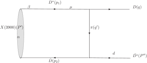
(I)                                (II)

Figure 2: strong decay of molecular state.

The corresponding Feynman diagrams are shown in Fig.2. Generally the intermediate mesons should include $\rho$, $\omega$, $\pi$ and $\sigma$. However for an $I=1$ molecular state the contributions from $\rho$ and $\omega$ nearly cancel each other as discussed in Ref.Guo:2007mm . In terms of the vertex function presented in the attached appendix, the hadronic matrix element corresponding to the diagrams in Fig.2 is written as

$$\mathcal{A}_{2}=i\frac{1}{(2\pi)^{4}}\int d^{4}p_{1}\frac{H_{A_{01}}S^{2(a)}_{d\alpha}+H_{A_{10}}S^{2(b)}_{d\alpha}}{N_{1}N_{1}^{\prime}N_{2}}\epsilon_{1}^{d}\epsilon^{\alpha}$$ (10)

with

$$S^{2(a)}_{d\alpha}=\frac{g_{{}_{\sigma DD}}g_{{}_{\sigma D^{*}D^{*}}}}{\sqrt{2}}g_{\alpha\beta}g^{\mu\beta}g_{d\mu}\mathcal{F}(m_{1},p_{1})\mathcal{F}(m_{2},p_{2})\mathcal{F}^{2}(m_{\sigma},q^{\prime}),$$

$$S_{d\alpha}^{2(b)}=\frac{-g_{{}_{\pi DD^{*}}}g_{{}_{\pi DD^{*}}}}{\sqrt{2}}g_{\alpha\beta}g^{\mu\beta}(-q_{\mu}+q^{\prime}{\mu})(p_{2d}+q^{\prime}_{d})\mathcal{F}(m_{1},p_{1})\mathcal{F}(m_{2},p_{2})\mathcal{F}^{2}(m_{D},q^{\prime}).$$ (11)

Carrying out the integral, $h_{A}\hat{S}_{d\alpha}$ is decomposed into

$${F_{21}}g_{d\alpha}+{F_{22}}P^{\prime}_{d}P^{\prime\prime}_{\alpha},$$ (12)

with

$$F_{21} =\frac{g_{{}_{\sigma DD}}g_{{}_{\sigma D^{*}D^{*}}}}{\sqrt{2}}\mathcal{F}(m_{1},p_{1})\mathcal{F}(m_{2},p_{2})\mathcal{F}^{2}(m_{\sigma},q^{\prime})+\sqrt{2}g_{{}_{\pi DD^{*}}}g_{{}_{\pi DD^{*}}}\,{A_{1}^{(2)}}$$

$$\mathcal{F}(m_{1},p_{1})\mathcal{F}(m_{2},p_{2})\mathcal{F}^{2}(m_{\pi},q^{\prime})$$

$$F_{22} =\sqrt{2}g_{{}_{\pi DD^{*}}}g_{{}_{\pi DD^{*}}}\,(-2+{A_{1}^{(1)}}+3\,{A_{2}^{(1)}}+{A_{2}^{(2)}}-2\,{A_{3}^{(2)}}-{A_{4}^{(2)}})$$ (13)

$$\mathcal{F}(m_{1},p_{1})\mathcal{F}(m_{2},p_{2})\mathcal{F}^{2}(m_{\pi},q^{\prime}).$$

Similar to the definitions in Eq.II.1 the amplitude then is

$$\mathcal{A}_{2} =f_{21}\epsilon\cdot\epsilon_{1}+f_{22}{P^{\prime\prime}\cdot\epsilon P^{\prime}\cdot\epsilon_{1}}.$$ (14)

III The strong decays of $Z_{c}(4030)$ which is assumed to be a $1^{+}$ molecular state of $D^{*}\bar{D}^{*}$

Now let us consider strong decays of $Z_{c}(4030)$ which is assumed to be a $D^{*}\bar{D}^{*}$ molecular state. Similar to what we have done for $Z_{c}(3900)$, we calculate the decay rates for $Z_{c}(4030)\rightarrow J/\psi\pi$, $Z_{c}(4030)\rightarrow\psi^{\prime}\pi$, $Z_{c}(4030)\rightarrow\rho\eta_{c}$, $Z_{c}(4030)\rightarrow D\bar{D}^{*}$, and one more channel: $Z_{c}(4030)\rightarrow D^{*}\bar{D}^{*}$ which is open at the energy of 4030 MeV.

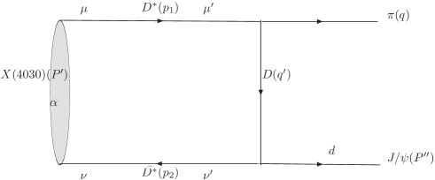
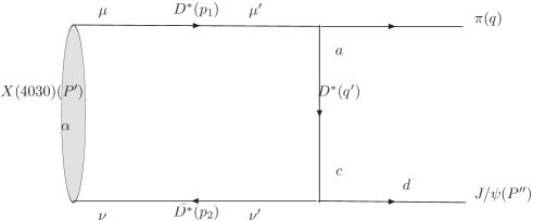
(a)                                (b)
+the Figures exchanged the final states

Figure 3: strong decay $Z_{c}(4030)\rightarrow J/\psi\pi$

III.1 $Z_{c}(4030)\rightarrow J/\psi\pi\,(\rho\eta_{c}\,{\rm or}\,\psi^{\prime}\pi)$

The Feynman diagrams are shown in Fig.3. In terms of the vertex function given in the appendix, the hadronic matrix element is

$$\mathcal{A}_{31}=i\frac{1}{(2\pi)^{4}}\int d^{4}p_{1}\frac{H_{A_{1}}}{N_{1}N_{1}^{\prime}N_{2}}(S^{3(a)}_{d\alpha}+S^{3(b)}_{d\alpha})\epsilon_{1}^{d}\epsilon^{\alpha},$$ (15)

where

$$S_{d\alpha}^{3(a)}=g_{{}_{\psi DD^{*}}}g_{{}_{\pi DD^{*}}}\varepsilon_{\mu\nu\alpha\beta}g^{\mu\mu^{\prime}}(2q_{\mu^{\prime}}-p_{1\mu^{\prime}})P^{\prime\beta}g^{\nu\nu^{\prime}}\varepsilon_{ab\nu^{\prime}d}P^{\prime\prime a}p_{2}^{b}\mathcal{F}(m_{1},p_{1})\mathcal{F}(m_{2},p_{2})\mathcal{F}^{2}(m_{D},q^{\prime}),$$

and $S_{d\alpha}^{3(b)}=g_{{}_{\psi D^{*}D^{*}}}g_{{}_{\pi D^{*}D^{*}}}\varepsilon_{\mu\nu\alpha\beta}g^{\mu\mu^{\prime}}P^{\prime\beta}g^{\nu\nu^{\prime}}\varepsilon_{\omega\mu^{\prime}\rho a}p_{1}^{\omega}q^{\prime\rho}g^{ac}[(q^{\prime}-p_{2})_{d}g_{c\nu^{\prime}}-q^{\prime}_{\nu}g_{dc}+p_{2c}g_{d\nu^{\prime}}]$ $\mathcal{F}(m_{1},p_{1})\mathcal{F}(m_{2},p_{2})\mathcal{F}^{2}(m_{D^{*}},q^{\prime}).$ Carrying out the integration and making the required replacements, we have

$$h_{A_{1}}(\hat{S}^{3(a)}_{d\alpha}+\hat{S}^{3(b)}_{d\alpha})={F_{31}}g_{d\alpha}+{F_{32}}P^{\prime}_{d}P^{\prime\prime}_{\alpha},$$ (16)

with

$${F_{31}}= \frac{g_{{}_{\psi DD^{*}}}g_{{}_{\pi DD^{*}}}h_{A_{1}}}{4}[2\,{{M^{\prime}}}^{4}-{A_{1}^{(1)}}\,{{M^{\prime}}}^{4}-3\,{A_{2}^{(1)}}\,{{M^{\prime}}}^{4}+3\,{A_{2}^{(2)}}\,{{M^{\prime}}}^{4}+4\,{A_{3}^{(2)}}\,{{M^{\prime}}}^{4}+{A_{4}^{(2)}}\,{{M^{\prime}}}^{4}$$

$$-4\,{{M^{\prime}}}^{2}\,{{M^{\prime\prime}}}^{2}+2\,{A_{1}^{(1)}}\,{{M^{\prime}}}^{2}\,{{M^{\prime\prime}}}^{2}+6\,{A_{2}^{(1)}}\,{{M^{\prime}}}^{2}\,{{M^{\prime\prime}}}^{2}+10\,{A_{2}^{(2)}}\,{{M^{\prime}}}^{2}\,{{M^{\prime\prime}}}^{2}-4\,{A_{3}^{(2)}}\,{{M^{\prime}}}^{2}\,{{M^{\prime\prime}}}^{2}$$

$$-2\,{A_{4}^{(2)}}\,{{M^{\prime}}}^{2}\,{{M^{\prime\prime}}}^{2}+2\,{{M^{\prime\prime}}}^{4}-{A_{1}^{(1)}}\,{{M^{\prime\prime}}}^{4}-3\,{A_{2}^{(1)}}\,{{M^{\prime\prime}}}^{4}+3\,{A_{2}^{(2)}}\,{{M^{\prime\prime}}}^{4}+{A_{4}^{(2)}}\,{{M^{\prime\prime}}}^{4}$$

$$+4\,{A_{1}^{(2)}}\,({{M^{\prime}}}^{2}+{{M^{\prime\prime}}}^{2}-{q^{2}})-2\,{{m_{1}}}^{2}\,({{M^{\prime}}}^{2}+{{M^{\prime\prime}}}^{2}-{q^{2}})-4\,{{M^{\prime}}}^{2}\,{q^{2}}+2\,{A_{1}^{(1)}}\,{{M^{\prime}}}^{2}\,{q^{2}}$$

$$+6\,{A_{2}^{(1)}}\,{{M^{\prime}}}^{2}\,{q^{2}}-4\,{A_{2}^{(2)}}\,{{M^{\prime}}}^{2}\,{q^{2}}-4\,{A_{3}^{(2)}}\,{{M^{\prime}}}^{2}\,{q^{2}}-4\,{{M^{\prime\prime}}}^{2}\,{q^{2}}+2\,{A_{1}^{(1)}}\,{{M^{\prime\prime}}}^{2}\,{q^{2}}$$

$$+6\,{A_{2}^{(1)}}\,{{M^{\prime\prime}}}^{2}\,{q^{2}}-4\,{A_{2}^{(2)}}\,{{M^{\prime\prime}}}^{2}\,{q^{2}}+2\,{{q^{4}}}-{A_{1}^{(1)}}\,{{q^{4}}}-3\,{A_{2}^{(1)}}\,{{q^{4}}}+{A_{2}^{(2)}}\,{{q^{4}}}-{A_{4}^{(2)}}\,{{q^{4}}}$$

$$-2\,{{M^{\prime}}}^{2}\,(-{{M_{0}^{\prime}}}^{2}+{{M^{\prime}}}^{2})\,{x_{1}}+2\,({{M_{0}^{\prime}}}^{2}-{{M^{\prime}}}^{2})\,{{M^{\prime\prime}}}^{2}\,{x_{1}}+2\,(-{{M_{0}^{\prime}}}^{2}+{{M^{\prime}}}^{2})\,{q^{2}}\,{x_{1}}]$$

$$\mathcal{F}(m_{1},p_{1})\mathcal{F}(m_{2},p_{2})\mathcal{F}^{2}(m_{D},q^{\prime})$$

$$+\frac{g_{{}_{\psi D^{*}D^{*}}}g_{{}_{\pi D^{*}D^{*}}}h_{A_{1}}}{2}\{6\,{A_{1}^{(2)}}\,({{M^{\prime}}}^{2}-{{M^{\prime\prime}}}^{2}+{q^{2}})-({A_{1}^{(1)}}+{A_{2}^{(2)}})\,[{{M^{\prime}}}^{4}+{({{M^{\prime\prime}}}^{2}-{q^{2}})}^{2}$$

$$-2\,{{M^{\prime}}}^{2}\,({{M^{\prime\prime}}}^{2}+{q^{2}})]\}\mathcal{F}(m_{1},p_{1})\mathcal{F}(m_{2},p_{2})\mathcal{F}^{2}(m_{D^{*}},q^{\prime})$$

$${F_{32}}= \frac{g_{{}_{\psi DD^{*}}}g_{{}_{\pi DD^{*}}}h_{A_{1}}}{2}[-4\,{A_{1}^{(2)}}+2\,{{m_{1}}}^{2}-2\,{{M^{\prime}}}^{2}+{A_{1}^{(1)}}\,{{M^{\prime}}}^{2}+3\,{A_{2}^{(1)}}\,{{M^{\prime}}}^{2}-3\,{A_{2}^{(2)}}\,{{M^{\prime}}}^{2}$$ (17)

$$-4\,{A_{3}^{(2)}}\,{{M^{\prime}}}^{2}-{A_{4}^{(2)}}\,{{M^{\prime}}}^{2}-2\,{{M^{\prime\prime}}}^{2}+{A_{1}^{(1)}}\,{{M^{\prime\prime}}}^{2}+3\,{A_{2}^{(1)}}\,{{M^{\prime\prime}}}^{2}-3\,{A_{2}^{(2)}}\,{{M^{\prime\prime}}}^{2}$$

$$-{A_{4}^{(2)}}\,{{M^{\prime\prime}}}^{2}+2\,{q^{2}}-{A_{1}^{(1)}}\,{q^{2}}-3\,{A_{2}^{(1)}}\,{q^{2}}+{A_{2}^{(2)}}\,{q^{2}}-{A_{4}^{(2)}}\,{q^{2}}-2\,{{M_{0}^{\prime}}}^{2}\,{x_{1}}+2\,{{M^{\prime}}}^{2}\,{x_{1}}]$$

$$\mathcal{F}(m_{1},p_{1})\mathcal{F}(m_{2},p_{2})\mathcal{F}^{2}(m_{D},q^{\prime})$$

$$+g_{{}_{\psi D^{*}D^{*}}}g_{{}_{\pi D^{*}D^{*}}}h_{A_{1}}[6\,{A_{1}^{(2)}}+{A_{1}^{(1)}}\,(-7\,{{M^{\prime}}}^{2}+{{M^{\prime\prime}}}^{2}-{q^{2}})+{A_{2}^{(2)}}\,(9\,{{M^{\prime}}}^{2}+{{M^{\prime\prime}}}^{2}-{q^{2}})]$$

$$\mathcal{F}(m_{1},p_{1})\mathcal{F}(m_{2},p_{2})\mathcal{F}^{2}(m_{D^{*}},q^{\prime}).$$

We define the form factors as following

$${f_{31}}(m_{1},m_{2})=\frac{1}{32\pi^{3}}\int dx_{2}d^{2}p_{\perp}\frac{F_{31}}{x_{2}\hat{N_{1}}\hat{N_{1}^{\prime}}},$$

$${f_{32}}(m_{1},m_{2})=\frac{1}{32\pi^{3}}\int dx_{2}d^{2}p_{\perp}\frac{F_{32}}{x_{2}\hat{N_{1}}\hat{N_{1}^{\prime}}},$$ (18)

which will be numerically evaluated in next section.

With these form factors the amplitude is obtained as

$$\mathcal{A}_{31} ={f_{31}}(m_{1},m_{2})\epsilon\cdot\epsilon_{1}+{f_{32}}(m_{1},m_{2}){P^{\prime\prime}\cdot\epsilon P^{\prime}\cdot\epsilon_{1}}.$$ (19)

Similarly, the amplitude corresponding the Feynman diagrams which are obtained by switching around the mesons in the final states can be easily obtained by exchanging $m_{1}$ and $m_{2}$. The total amplitude is

$$\mathcal{A}_{3} =\mathcal{A}_{31}+\mathcal{A}_{32}$$ (20)

$$=[f_{31}(m_{1},m_{2})+f_{31}(m_{2},m_{1})]\epsilon\cdot\epsilon_{1}+[f_{32}(m_{1},m_{2})+f_{32}(m_{2},m_{1})]{P^{\prime\prime}\cdot\epsilon P^{\prime}\cdot\epsilon_{1}}$$

$$=g_{31}\epsilon\cdot\epsilon_{1}+g_{32}{P^{\prime\prime}\cdot\epsilon P^{\prime}\cdot\epsilon_{1}}.$$

III.2 $Z_{c}(4030)\rightarrow D\bar{D}^{*}$

Since there does not exist an effective coupling of $\sigma$ with a psedoscalar and a vector, only the Feynman diagram with intermediate $\pi$ can contribute.

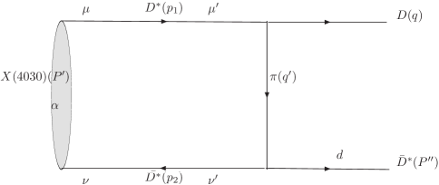
Figure 4: strong decay of molecular state.

In terms of the vertex function, the hadronic matrix element corresponding to (a) and (b) of Fig.4 is

$$\mathcal{A}_{4}=i\frac{1}{(2\pi)^{4}}\int d^{4}p_{1}\frac{H_{A_{1}}}{N_{1}N_{1}^{\prime}N_{2}}S_{d\alpha}\epsilon_{1}^{d}\epsilon^{\alpha}$$ (21)

where

$$S_{d\alpha}=-g_{{}_{\pi DD^{*}}}g_{{}_{\pi D^{*}D^{*}}}\varepsilon_{\mu\nu\alpha\beta}g^{\mu\mu^{\prime}}(-2q_{\mu^{\prime}}+p_{1\mu^{\prime}})P^{\prime\beta}g^{\nu\nu^{\prime}}\varepsilon_{ab\nu^{\prime}d}P^{\prime\prime a}p_{2}^{b}\mathcal{F}(m_{1},p_{1})\mathcal{F}(m_{2},p_{2})\mathcal{F}^{2}(m_{\pi},q^{\prime}),$$

Carrying out the integration and making the replacements, we have

$$\hat{S}_{d\alpha}={F_{41}}g_{d\alpha}+{F_{42}}P^{\prime}_{d}P^{\prime\prime}_{\alpha},$$ (22)

with

$${F_{41}}= \frac{g_{{}_{\pi DD^{*}}}g_{{}_{\pi D^{*}D^{*}}}h_{A_{1}}}{4}[-2\,{{M^{\prime}}}^{4}+{A_{1}^{(1)}}\,{{M^{\prime}}}^{4}+3\,{A_{2}^{(1)}}\,{{M^{\prime}}}^{4}-3\,{A_{2}^{(2)}}\,{{M^{\prime}}}^{4}-4\,{A_{3}^{(2)}}\,{{M^{\prime}}}^{4}-{A_{4}^{(2)}}\,{{M^{\prime}}}^{4}$$

$$+4\,{{M^{\prime}}}^{2}\,{{M^{\prime\prime}}}^{2}-2\,{A_{1}^{(1)}}\,{{M^{\prime}}}^{2}\,{{M^{\prime\prime}}}^{2}-6\,{A_{2}^{(1)}}\,{{M^{\prime}}}^{2}\,{{M^{\prime\prime}}}^{2}-10\,{A_{2}^{(2)}}\,{{M^{\prime}}}^{2}\,{{M^{\prime\prime}}}^{2}+4\,{A_{3}^{(2)}}\,{{M^{\prime}}}^{2}\,{{M^{\prime\prime}}}^{2}$$

$$+2\,{A_{4}^{(2)}}\,{{M^{\prime}}}^{2}\,{{M^{\prime\prime}}}^{2}-2\,{{M^{\prime\prime}}}^{4}+{A_{1}^{(1)}}\,{{M^{\prime\prime}}}^{4}+3\,{A_{2}^{(1)}}\,{{M^{\prime\prime}}}^{4}-3\,{A_{2}^{(2)}}\,{{M^{\prime\prime}}}^{4}-{A_{4}^{(2)}}\,{{M^{\prime\prime}}}^{4}$$

$$-4\,{A_{1}^{(2)}}\,({{M^{\prime}}}^{2}+{{M^{\prime\prime}}}^{2}-{q^{2}})+2\,{{m_{1}^{\prime}}}^{2}\,({{M^{\prime}}}^{2}+{{M^{\prime\prime}}}^{2}-{q^{2}})+4\,{{M^{\prime}}}^{2}\,{q^{2}}-2\,{A_{1}^{(1)}}\,{{M^{\prime}}}^{2}\,{q^{2}}$$

$$-6\,{A_{2}^{(1)}}\,{{M^{\prime}}}^{2}\,{q^{2}}+4\,{A_{2}^{(2)}}\,{{M^{\prime}}}^{2}\,{q^{2}}+4\,{A_{3}^{(2)}}\,{{M^{\prime}}}^{2}\,{q^{2}}+4\,{{M^{\prime\prime}}}^{2}\,{q^{2}}-2\,{A_{1}^{(1)}}\,{{M^{\prime\prime}}}^{2}\,{q^{2}}$$

$$-6\,{A_{2}^{(1)}}\,{{M^{\prime\prime}}}^{2}\,{q^{2}}+4\,{A_{2}^{(2)}}\,{{M^{\prime\prime}}}^{2}\,{q^{2}}-2\,q^{4}+{A_{1}^{(1)}}\,q^{4}+3\,{A_{2}^{(1)}}\,q^{4}$$

$$-{A_{2}^{(2)}}\,q^{4}+{A_{4}^{(2)}}\,q^{4}+2\,(-{{M_{0}^{\prime}}}^{2}+{{M^{\prime}}}^{2})\,({{M^{\prime}}}^{2}+{{M^{\prime\prime}}}^{2}-{q^{2}})\,{x_{1}}]\mathcal{F}(m_{1},p_{1})\mathcal{F}(m_{2},p_{2})\mathcal{F}^{2}(m_{\pi},q^{\prime})$$

$${F_{42}}= \frac{g_{{}_{\pi DD^{*}}}g_{{}_{\pi D^{*}D^{*}}}h_{A_{1}}}{2}[4\,{A_{1}^{(2)}}-2\,{{m_{1}}}^{2}+(2-{A_{1}^{(1)}}-3\,{A_{2}^{(1)}}+3\,{A_{2}^{(2)}}+{A_{4}^{(2)}})\,{{M^{\prime\prime}}}^{2}+(-2+{A_{1}^{(1)}}+$$ (23)

$$3\,{A_{2}^{(1)}}-{A_{2}^{(2)}}+{A_{4}^{(2)}})\,{q^{2}}+{{M^{\prime}}}^{2}\,(2-{A_{1}^{(1)}}-3\,{A_{2}^{(1)}}+3\,{A_{2}^{(2)}}+4\,{A_{3}^{(2)}}+{A_{4}^{(2)}}-2\,{x_{1}})$$

$$+2\,{{M_{0}^{\prime}}}^{2}\,{x_{1}}]\mathcal{F}(m_{1},p_{1})\mathcal{F}(m_{2},p_{2})\mathcal{F}^{2}(m_{\pi},q^{\prime}).$$

The amplitude can be eventually reached as

$$\mathcal{A}_{4} =f_{41}\epsilon\cdot\epsilon_{1}+f_{42}{P^{\prime\prime}\cdot\epsilon P^{\prime}\cdot\epsilon_{1}}.$$ (24)

III.3 $Z_{c}(4030)\rightarrow D^{*}\bar{D}^{*}$

For this decay mode there are two Feynman diagrams which are induced by exchanging $\pi$ and $\sigma$ between the two constituents $D^{*}$ and $\bar{D}^{*}$, making contribution.

(a)                                (b)

Figure 5: strong decay of molecular state.

In terms of the vertex function, the hadronic matrix element corresponding to diagrams (a) and (b) of Fig.5 is

$$\mathcal{A}_{5}=i\frac{1}{(2\pi)^{4}}\int d^{4}p_{1}\frac{H_{A_{1}}}{N_{1}N_{1}^{\prime}N_{2}}(S^{5(a)}_{df\alpha}+S^{5(b)}_{df\alpha})\epsilon_{1}^{d}\epsilon_{2}^{f}\epsilon^{\alpha}$$ (25)

$$S^{5(a)}_{df\alpha}=g_{{}_{\pi D^{*}D^{*}}}g_{{}_{\pi D^{*}D^{*}}}\varepsilon_{\mu\nu\alpha\beta}\varepsilon_{\rho\mu^{\prime}\omega f}\varepsilon_{adb\nu^{\prime}}g^{\mu\mu^{\prime}}g^{\nu\nu^{\prime}}P^{\prime\beta}(p_{1\rho})q_{\nu}P^{\prime\prime a}p_{2}^{b}\mathcal{F}(m_{1},p_{1})\mathcal{F}(m_{2},p_{2})\mathcal{F}^{2}(m_{\pi},q^{\prime}),$$

$$S^{5(b)}_{df\alpha}=g_{{}_{\sigma D^{*}D^{*}}}g_{{}_{\sigma D^{*}D^{*}}}\varepsilon_{\mu\nu\alpha\beta}g^{\mu\mu^{\prime}}g^{\nu\nu^{\prime}}P^{\prime\beta}g^{f\mu^{\prime}}g^{d\nu^{\prime}}\mathcal{F}(m_{1},p_{1})\mathcal{F}(m_{2},p_{2})\mathcal{F}^{2}(m_{\pi},q^{\prime}).$$ (26)

carrying the integration and making the replacement, one has

$$\hat{S}^{5(a)}_{df\alpha}+\hat{S}^{5(b)}_{df\alpha}={F_{51}}\varepsilon_{df\mu\nu}P^{\prime\mu}P^{\prime\prime\nu}P^{\prime\prime\alpha}+{F_{52}}\varepsilon_{df\alpha\beta}P^{\prime}_{\beta},$$ (27)

with

$${F_{51}}= 2g_{{}_{\pi D^{*}D^{*}}}g_{{}_{\pi D^{*}D^{*}}}h_{A_{1}}A_{1}^{1}(A_{1}^{1}+A_{2}^{1}-1)\mathcal{F}(m_{1},p_{1})\mathcal{F}(m_{2},p_{2})\mathcal{F}^{2}(m_{\pi},q^{\prime})$$

$${F_{52}}= g_{{}_{\sigma D^{*}D^{*}}}g_{{}_{\sigma D^{*}D^{*}}}h_{A_{1}}\mathcal{F}(m_{1},p_{1})\mathcal{F}(m_{2},p_{2})\mathcal{F}^{2}(m_{\sigma},q^{\prime}).$$ (28)

The amplitude is

$$\mathcal{A}_{5} ={f_{51}}\varepsilon_{df\mu\nu}P^{\prime\mu}P^{\prime\prime\nu}P^{\prime\prime\alpha}\epsilon_{\alpha}\epsilon_{1d}\epsilon_{2f}+{f_{52}}\varepsilon_{df\alpha\beta}P^{\prime}_{\beta}\epsilon_{\alpha}\epsilon_{1d}\epsilon_{2f}.$$ (29)

where the expressions of $f_{51}$ and $f_{52}$ are similar to Eq.II.1 and Eq.III.1.

IV numerical results

In this section we present our theoretical predictions on the decay rates of the concerned modes. The key point is to calculate the corresponding form factors we deduced in last section. Those formulas involve many parameters which need to be priori fixed. We use the BES dada 3.899 GeVAblikim:2013mio as the mass of $Z_{c}(3900)$ and the mass of $Z_{c}(4030)$ is assigned to be 4.03 GeV. The masses of the decay products and intermediate mesons are set as $m_{J/\psi}=3.096$ GeV, $m_{\psi^{\prime}}=3.686$ GeV, $m_{\eta_{c}}=2.981$ GeV, $m_{\rho}=0.77$ GeV, $m_{\pi}=0.139$ GeV, $m_{D}=1.869$ GeV, $m_{D^{*}}=2.007$ GeV and $m_{\sigma}=0.5$ GeV taken from Ref.PDG12 . In Refs.Haglin:1999xs ; Oh:2000qr the coupling constants $g_{{}_{\pi DD^{*}}}$ and $g_{{}_{\pi D^{*}D^{*}}}$ were fixed to be 8.8 and 9.08 GeV^-1 respectively. For the coupling of $\psi D^{(*)}D^{(*)}$, $\psi DD^{*}$ and $\psi D^{*}D^{*}$ there exists a simple, but approximate relation $g_{{}_{\psi DD}}=m_{D}g_{{}_{\psi DD^{*}}}=g_{{}_{\psi D^{*}D^{*}}}$Deandrea:2003pv ; Meng:2007cx and $g_{{}_{\psi DD}}=g_{{}_{\psi D^{*}D^{*}}}=8.0$Lin:1999ad , so we can fix $g_{{}_{\psi DD^{*}}}=4.28$ GeV^-1. In the heavy quark limit the relation $g_{{}_{\eta_{c}D^{*}D}}=m_{D}g_{{}_{\eta_{c}D^{*}D^{*}}}=g_{{}_{\psi DD}}$ should exist. The coupling constant $g_{{}_{\rho DD}}$ and $g_{{}_{\rho D^{*}D^{*}}}$ are set to be 3Guo:2007mm in our calculation and $g_{{}_{\rho DD^{*}}}=3$ GeV^-1 is adopted. $g_{{}_{\sigma D^{*}D^{*}}}=2m_{D^{*}}g_{\sigma}$ and $g_{{}_{\sigma DD}}=2m_{D}g_{\sigma}$ with $g_{\sigma}=0.76$Lee:2009hy are also reasonable approximations. $\Lambda$ in the vertex $\mathcal{F}$ is a cutoff parameter which was suggested to set as 0.88 GeV to 1.1 GeV in Ref.Meng:2007cx and we will use both of the values in our calculation and compare the results. The other parameter $\beta$ in the wavefunction is not very clear so far and its value is estimated to be near or smaller than the number of $\beta$ for the wavefunction of $J/\psi$ which is fixed to be 0.631 GeV^-1 in Ref.Ke:2011jf .

Since we derive the form factors in the frame of $q^{+}=0$ ( $q^{2}<0$) i.e. in space-like region, we extend these form factors to the time-like region according to the normal procedure provided in literatures. Then letting $q^{2}$ take the value of $m^{2}$ , the physical form factors are obtained. In Ref.Cheng:2003sm a three-parameter form was suggested as

$$F(q^{2})=\frac{F(0)}{\left[1-a\left(\frac{q^{2}}{M_{\Lambda_{b}}^{2}}\right)+b\left(\frac{q^{2}}{M_{\Lambda_{b}}^{2}}\right)^{2}\right]}.$$ (30)

However we find the form Eq.30 does not fit the numerical values satisfactorily (see the figures), so instead, we employ a polynomial

$$F(q^{2})=F(0)\left[1+a\left(\frac{q^{2}}{M_{\Lambda_{b}}^{2}}\right)+b\left(\frac{q^{2}}{M_{\Lambda_{b}}^{2}}\right)^{2}+c\left(\frac{q^{2}}{M_{\Lambda_{b}}^{2}}\right)^{3}+d\left(\frac{q^{2}}{M_{\Lambda_{b}}^{2}}\right)^{4}\right].$$ (31)

The resultant form factors and the effective coupling constants are listed in table 1.

Table 1: The form factors given in the five-parameter form ($\Lambda=0.88$ GeV, $\beta=0.631$ GeV^-1). The numbers above the horizontal line correspond to $Z_{c}(3900)$ and those numbers below the line correspond to $Z_{c}(4030)$. The definitions of the form factors are given in last section.

$F$	$F(0)$	$a$	$b$	$c$	$d$	$F$	$F(0)$	$a$	$b$	$c$	$d$
$g_{11}^{J/\psi\pi}$	-1.05	10.59	17.83	14.73	4.90	$g_{12}^{J/\psi\pi}$	-1.16	2.33	3.21	2.51	0.82
$g_{11}^{\psi(2S)\pi}$	-4.24	9.32	18.271	16.57	5.82	$g_{12}^{J/\psi(2S)\pi}$	-4.35	3.18	5.33	4.67	1.63
$g_{11}^{\rho\eta_{c}}$	0.065	- 6.81	-9.34	-6.769	-2.10	$g_{12}^{J/\rho\eta_{c}}$	-0.083	1.66	1.85	1.30	0.40
$f_{21}$	0.052	5.34	12.57	13.43	5.27	$f_{22}$	0.39	5.72	13.89	15.12	5.99
$g_{31}^{J/\psi\pi}$	2.90	-10.39	-21.90	-20.54	-7.53	$g_{32}^{J/\psi\pi}$	0.64	3.23	5.05	4.26	1.49
$g_{31}^{\psi(2S)\pi}$	-0.84	-59.48	-148.71	-155.46	-60.64	$g_{32}^{\psi(2S)\pi}$	-1.30	3.89	6.86	6.20	2.25
$g_{31}^{\rho\eta_{c}}$	-0.46	0.15	-0.16	-0.17	-0.06	$g_{32}^{J/\rho\eta_{c}}$	-0.011	5.80	8.78	6.99	2.34
$f_{41}$	-0.28	0.031	-4.79	-7.81	-3.76	$f_{42}$	-0.26	5.25	12.676	14.20	5.89
$f_{51}$	0.074	5.35	12.91	14.42	5.96	$f_{52}$	-$0.053$	5.14	12.04	13.23	5.42

Table 2: The decay widths of some modes ($\Lambda=0.88$ GeV, $\beta=0.631$ GeV^-1).

decay mode	width(MeV)	decay mode	width(MeV)
$Z_{c}(3900)\rightarrow J/\psi\pi$	3.67	$Z_{c}(4030)\rightarrow J/\psi\pi$	17.85
$Z_{c}(3900)\rightarrow\psi(2S)\pi$	8.24	$Z_{c}(4030)\rightarrow\psi(2S)\pi$	0.30
$Z_{c}(3900)\rightarrow\rho\eta_{c}$	0.45	$Z_{c}(4030)\rightarrow\rho\eta_{c}$	0.30
$Z_{c}(3900)\rightarrow DD^{*}$	0.024	$Z_{c}(4030)\rightarrow DD^{*}$	0.23
-	-	$Z_{c}(4030)\rightarrow D^{*}D^{*}$	0.52

Table 3: The decay widths of some modes ($\Lambda=1.1$ GeV, $\beta=0.631$ GeV^-1).

decay mode	width(MeV)	decay mode	width(MeV)
$Z_{c}(3900)\rightarrow J/\psi\pi$	6.44	$Z_{c}(4030)\rightarrow J/\psi\pi$	35.08
$Z_{c}(3900)\rightarrow\psi(2S)\pi$	12.00	$Z_{c}(4030)\rightarrow\psi(2S)\pi$	0.66
$Z_{c}(3900)\rightarrow\rho\eta_{c}$	0.88	$Z_{c}(4030)\rightarrow\rho\eta_{c}$	0.53
$Z_{c}(3900)\rightarrow DD^{*}$	0.055	$Z_{c}(4030)\rightarrow DD^{*}$	0.62
-	-	$Z_{c}(4030)\rightarrow D^{*}D^{*}$	0.96

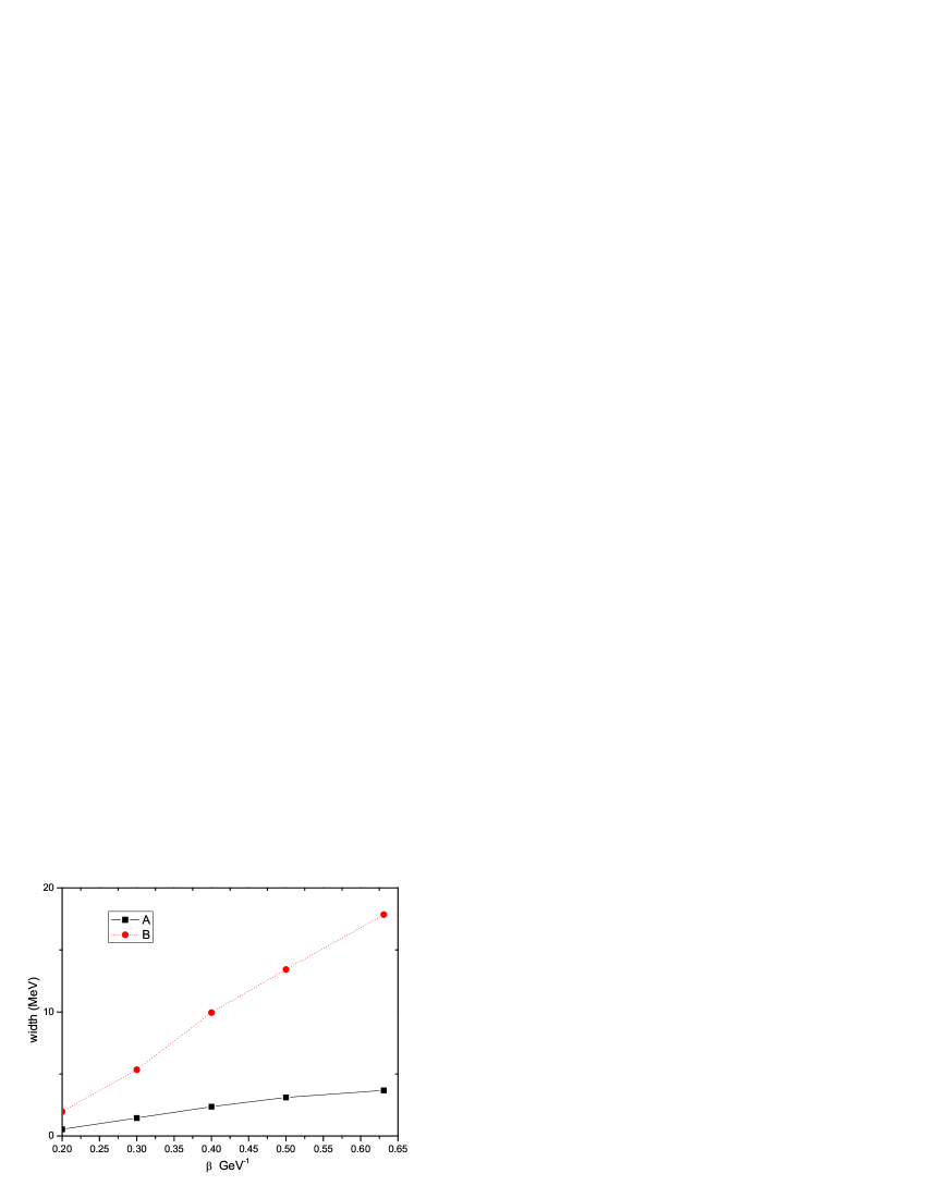
Figure 6: the dependence of $\Gamma(Z_{c}(3900)\rightarrow J/\psi\pi$) (A) and $\Gamma(Z_{c}(4030)\rightarrow J/\psi\pi$) (B) on $\beta$.

One can find if $Z_{c}(3900)$ is a molecular state of $D\bar{D}^{*}$ the partial width of $Z_{c}(3900)\rightarrow D\bar{D}^{*}$ is very small. For $Z_{c}(4030)$ both the partial widths $\Gamma(Z_{c}(4030)\rightarrow D^{*}\bar{D}^{*})$ $\Gamma(Z_{c}(4030)\rightarrow D\bar{D}^{*})$ are small, but sufficiently sizable to be measured.

In our calculation, we notice that the model parameters $\Lambda$ and $\beta$ can affect the numerical results sensitively. Since the $\beta$ is a model parameter which is closely related to the behavior of the wavefuctions of the concerned hadrons, we illustrate the dependence of $Z_{c}(3900)\rightarrow J/\psi\pi$ and $Z_{c}(4030)\rightarrow J/\psi\pi$ on $\beta$ in Fig.6. Line A and B in Fig.6 correspond to $Z_{c}(3900)$ and $Z_{c}(4030)$ respectively. In Ref.Dong:2013iqa the estimated $\Gamma(Z_{c}(3900)\rightarrow J/\psi\pi)$ is about 1 MeV which is smaller than our results.

V discussions and a tentative conclusion

In this work we calculate the decay rates of $Z_{c}(3900)$ to $J\psi\pi$, $\psi(2s)\pi$, $\eta_{c}\rho$ and $D^{*}\bar{D}^{*}$ in the LFM by assuming that $Z_{c}(3900)$ is a molecular state of $\frac{1}{\sqrt{2}}(D\bar{D}^{*}+D^{*}\bar{D})$. The numerical results are shown in tables II and III where we vary the model parameters $\Lambda$ to check the parameter dependence. Then in the same framework, we evaluate the decay rates of a postulated $Z_{c}(4030)$ which was predicted by VoloshinVoloshin:2013dpa according to the mass gap between $Z_{b}(10610)$ and $Z_{b}(10650)$. It is tempted to consider $Z_{c}(4030)$ as a molecular state of $D^{*}\bar{D}^{*}$. Very recently, the BES collaboration reports that two resonances $Z_{c}(4020)$ and $Z_{c}(4025)$ were observed Yuan . The resonance $Z_{c}(4020)$ is observed in the channel of $e^{+}e^{-}\to\pi Z_{c}(4020)\to\pi^{+}\pi^{-}h_{c}(1P)$ at CM energies of 4.26/4.36 GeV and the fit results are $M(4020)=(4021.8\pm 1.0\pm 2.5)$ MeV and $\Gamma(4020)=(5.7\pm 3.4\pm 1.1)$ MeV, whereas $Z_{c}(2025)$ is observed in the channel $e^{+}e^{-}\to\pi^{-}D^{*}\bar{D}^{*}$ at the CM energy of 4.26 GeV with the fit results of $N(4025)=(4026.3\pm 2.6\pm 3.7)$ MeV, $\Gamma(4025)=(24.8\pm 5.7\pm 7.7)$ MeV. Both of them are slightly lower than 4030 MeV. Since they are apart by only 2$\sigma$, one still may ask if they are the same resonance and the difference is due to experimental errors.The results of this work may help to clarify if they are indeed one resonance.

Our numerical results listed in tables II and III show that the decay rate of $Z_{c}(3900)\to J/\psi\pi$, which is the channel of first observing $Z_{c}(3900)$, is about a few MeV. But the decay $Z_{c}(3900)\to D\bar{D}^{*}({\rm or}D^{*}\bar{D})$ is much smaller than that for the $J/\psi$ final state. It is also noted that the rate of $Z_{c}(3900)\to\psi(2s)\pi$ is almost twice larger than that for $Z_{c}(3900)\to J/\psi\pi$. Even though the final state phase space of $\psi(2s)\pi$ is smaller than that for $J/\psi\pi$, the form factor for $Z_{c}\to\psi(2s)\pi$ is larger to result in the enhanced rate.

For the numerical computations we take 4030 MeV as the mass of $Z_{c}(4030)$ , but of course it is easy to adjust it into 4020 or 4025 MeV. Since the two resonances are waiting for further confirmation, we at present employ 4030 MeV as input, and the numerical results would be of significance even though not accurate. Our numerical results show that the tendency of the predicted decay rates for $Z_{c}(4030)$ are similar to that for $Z_{c}(3900)$.

The predicted rates are somehow sensitive to the model parameters, for example in tables II and III, we only change the value of $\Lambda$ from 0.88 GeV to 1.1 GeV which were determined by fitting data of different experiments, the rates are almost doubled. Fig.6 shows dependence of $\Gamma(Z_{c}(3900)\to J/\psi\pi)$ and $\Gamma(Z_{c}(4030)\to J/\psi\pi)$ on the $\beta-$value. Since the values of $\Lambda$ and $\beta$ are obtained by fitting data of experiments, we can only adjust those parameters within small ranges, so that the predictions with the model cannot be drastically changed. Namely, even though the predicted values may vary by a factor of two or even larger, the degree of magnitude remains the same.

Because the theoretical predictions are not fully accordant with the available data, although the data so far are not very accurate, we prefer to draw a tentative conclusion that the observed $Z_{c}(3900)$ and newly observed $Z_{c}(4020)$ and/or $Z_{c}(4025)$ are not molecular states of $D\bar{D}^{*}$ and $D^{*}\bar{D}^{*}$, but may be tetraquarks or mixtures of molecular states and tetraquarks. It is difficult to evaluate the decay rates of tetraquarks because there the non-perturbative QCD effects would dominate. In our later work, we will try to do it in terms of some reasonable models. Definitely further more accurate measurements on the decays of such exotic states: $Z_{b}$, $Z_{b}^{\prime}$, $Z_{c}$ and $Z_{c}^{\prime}$ are very badly needed.

Appendix A

Appendix B the vertex function of molecular state

Supposing $Z_{c}(3900)$ and $Z_{c}(4030)$ are molecular states which consists of $D$ and $\bar{D^{*}}$ and $D^{*}$ and $\bar{D^{*}}$ respectively. If the orbital angular momentum between the two components is zero, i.e. $l=0$, the total spin $S$ should be 0, 1 and 2 and total angular momentum $J$ also is 0, 1 and 2.

Similar to our previous works on baryons Ke:2007tg , we construct the vertex function of molecular in the same model. The wavefunction of a molecualr with total spin $J$ and momentum $P$ is

$$|X(P,J,J_{z})\rangle = \int\{d^{3}\tilde{p}_{1}\}\{d^{3}\tilde{p}_{2}\}\,2(2\pi)^{3}\delta^{3}(\tilde{P}-\tilde{p_{1}}-\tilde{p_{2}})$$ (32)

$$\times\sum_{\lambda_{1}}\Psi^{SS_{z}}(\tilde{p}_{1},\tilde{p}_{2},\lambda_{1},\lambda_{2})\mathcal{F}\left|\right.D^{(*)}(p_{1},\lambda_{1})\bar{D}^{*}(p_{2},\lambda_{2})\rangle,$$

with

$$\Psi^{SS_{z}}(\tilde{p}_{1},\tilde{p}_{2},\lambda_{1},\lambda_{2})= \left\langle\lambda_{1}\left|\mathcal{R}^{\dagger}_{M}(x_{1},k_{1\perp},m_{1})\right|s_{1}\right\rangle\left\langle\lambda_{2}\left|\mathcal{R}^{\dagger}_{M}(x_{2},k_{2\perp},m_{2})\right|s_{2}\right\rangle$$

$$\left\langle 1s_{1};1s_{2}\left|SS_{z}\right\rangle\langle SS_{z};00\left|JJ_{z}\right\rangle\varphi(x,k_{\perp})\right.,$$

where $\langle 1s_{1};1s_{2}|SS_{z}\rangle\langle SS_{z};00|JJ_{z}\rangle$ is the C-G coefficients and $s_{1},s_{2}$ are the spin projections of the constituents. These C-G coefficients can be rewrote as

$$\langle 1s_{1};00|SS_{z}\rangle\langle SS_{z};00|1J_{z}\rangle=A_{10}\epsilon_{1}(s_{1})\cdot\epsilon(J_{z})$$

$$\langle 00;1s_{2}|SS_{z}\rangle\langle SS_{z};00|1J_{z}\rangle=A_{01}\epsilon_{2}(s_{2})\cdot\epsilon(J_{z})$$

$$\langle 1s_{1};1s_{2}|SS_{z}\rangle\langle SS_{z};00|00\rangle=A_{0}\epsilon_{1}(s_{1})\cdot\epsilon_{2}(s_{2})$$

$$\langle 1s_{1};1s_{2}|SS_{z}\rangle\langle SS_{z};00|1J_{z}\rangle=A_{1}\varepsilon^{\mu\nu\alpha\beta}\epsilon_{1\mu}(s_{1})\epsilon_{2\nu}(s_{2})\epsilon_{\alpha}(J_{z})P_{\beta}$$

$$\langle 1s_{1};1s_{2}|SS_{z}\rangle\langle SS_{z};00|2J_{z}\rangle=A_{2}\epsilon_{1\mu}(s_{1})\epsilon_{2\nu}(s_{2})\epsilon^{\mu\nu}(J_{z})$$ (33)

with

$$A_{01}=\frac{\sqrt{3}m_{1}}{\sqrt{e_{1}^{2}+2m_{1}^{2}}},$$

$$A_{10}=\frac{\sqrt{3}m_{2}}{\sqrt{e_{2}^{2}+2m_{2}^{2}}},$$

$$A_{0}=\frac{2{m_{1}}{m_{2}}}{\sqrt{{M_{0}^{\prime}}^{4}-2{M_{0}^{\prime}}^{2}({m_{1}}^{2}+{m_{2}}^{2})+{m_{1}}^{4}+10{m_{1}}^{2}{m_{2}}^{2}+{m_{2}}^{4}}},$$

$$A_{1}=\frac{2\sqrt{3}{m_{1}}{m_{2}}}{\sqrt{{M^{\prime}}^{2}[4{e_{1}}^{2}{m_{2}}^{2}-4{e_{1}}{e_{2}}(-{M_{0}^{\prime}}^{2}+{m_{1}}^{2}+{m_{2}}^{2})+4{e_{2}}^{2}{m_{1}}^{2}+10{m_{1}}^{2}{m_{2}}^{2}-C_{A}]}},$$

$$A_{2}=\frac{\sqrt{120}{m_{1}}{m_{2}}}{\sqrt{4{e_{1}}^{2}(4{e_{2}}^{2}+7{m_{2}}^{2})+4{e_{1}}{e_{2}}(-{M_{0}^{\prime}}^{2}+{m_{1}}^{2}+{m_{2}}^{2})+28{e_{2}}^{2}{m_{1}}^{2}+54{m_{1}}^{2}{m_{2}}^{2}+C_{A}}},$$

$$C_{A}={M_{0}^{\prime}}^{4}-2{M_{0}^{\prime}}^{2}({m_{1}}^{2}+{m_{2}}^{2})+{m_{1}}^{4}+{m_{2}}^{4}.$$

A Melosh transformation brings the the matrix elements from the spin-projection-on-fixed-axes representation into the helicity representation and is explicitly written as

$$\left\langle\lambda_{2}\left|\mathcal{R}^{\dagger}_{M}(x_{2},k_{2\perp},m_{2})\right|s_{2}\right\rangle=\xi^{*}(\lambda_{2},m_{2})\cdot\xi(s_{2},m_{2}),$$

and

$$\left\langle\lambda_{1}\left|\mathcal{R}^{\dagger}_{M}(x_{1},k_{1\perp},m_{1})\right|s_{1}\right\rangle=\xi^{*}(\lambda_{1},m_{1})\cdot\xi(s_{1},m_{1}).$$

Following Refs. Jaus ; Cheng:2003sm , the Melosh transformed matrix can be expressed as

$$\langle\lambda_{1}|\mathcal{R}^{\dagger}_{M}(x_{1},k_{1\perp},m_{1})|s_{1}\rangle\langle\lambda_{2}|\mathcal{R}^{\dagger}_{M}(x_{2},k_{2\perp},m_{2})|s_{2}\rangle$$

$$\langle 1s_{1};1s_{2}|SS_{z}\rangle\langle SS_{z};00|JJ_{z}\rangle$$

$$=A_{1}\varepsilon^{\mu\nu\alpha\beta}\epsilon_{1\mu}(\lambda_{1})\epsilon_{2\nu}(\lambda_{2})\epsilon_{\alpha}(J_{z})P_{\beta},$$ (34)

so the wavefunction of $1^{+}$ molecular state of $D^{(*)}\bar{D}^{*}$

$$\Psi^{SS_{z}}(\tilde{p}_{1},\tilde{p}_{2},\lambda_{1},\lambda_{2}) =A_{1}\varphi(x,k_{\perp})\varepsilon^{\mu\nu\alpha\beta}\epsilon_{1\mu}(\lambda_{1})\epsilon_{2\nu}(\lambda_{2})\epsilon_{\alpha}(J_{z})P_{\beta}$$ (35)

$$=h_{A_{1}}^{\prime}\varepsilon^{\mu\nu\alpha\beta}\epsilon_{1\mu}(\lambda_{1})\epsilon_{2\nu}(\lambda_{2})\epsilon_{\alpha}(J_{z})P_{\beta},$$

with $\varphi=4(\frac{\pi}{\beta^{2}})^{3/4}\frac{e_{1}e_{2}}{x_{1}x_{2}M_{0}}{\rm exp}(\frac{-\mathbf{k}^{2}}{2\beta^{2}})$.

Similarly the wavefunction of $1^{+}$ molecular state of $D\bar{D}^{*}$

$$\Psi^{SS_{z}}(\tilde{p}_{1},\tilde{p}_{2},\lambda_{1},\lambda_{2}) =A\varphi(x,k_{\perp})\epsilon_{1\mu}(\lambda_{1})\cdot\epsilon_{\alpha}(J_{z})$$ (36)

$$=h_{A_{1}}^{\prime}\epsilon_{1\mu}(\lambda_{1})\cdot\epsilon_{\alpha}(J_{z}).$$

and normalization of the state is $X(P,J,J_{z})\rangle$ ,

$$\langle X(P^{\prime},J^{\prime},J_{z}^{\prime})|X(P,J,J_{z})\rangle=2(2\pi)^{3}P^{+}\delta^{3}(\tilde{P}^{\prime}-\tilde{P})\delta_{J^{\prime}J}\delta_{J^{\prime}_{z}J_{z}}.$$ (37)

All other notations can be found in Ref.Ke:2007tg .

Appendix C the effective vertices

the effective vertices can be found in Haglin:1999xs ; Oh:2000qr ; Lin:1999ad ; Deandrea:2003pv ; Meng:2007cx ,

$$\mathcal{L}_{\pi DD^{*}}=ig_{{}_{\pi DD^{*}}}(D^{*\mu}\partial_{\mu}\pi\bar{D}-\partial^{\mu}D\pi\bar{D}^{*}_{\mu}+h.c.),$$ (38)

$$\mathcal{L}_{\pi D^{*}D^{*}}=-g_{{}_{\pi D^{*}D^{*}}}\varepsilon^{\mu\nu\alpha\beta}\partial^{\mu}\bar{D}^{*}_{\nu}\pi\partial_{\alpha}D^{*\beta},$$ (39)

$$\mathcal{L}_{\psi DD}=ig_{{}_{\psi DD}}\psi_{\mu}(\partial^{\mu}D\bar{D}-D\partial^{\mu}\bar{D}),$$ (40)

$$\mathcal{L}_{\psi DD^{*}}=-g_{{}_{\psi DD^{*}}}\varepsilon^{\mu\nu\alpha\beta}\partial^{\mu}\psi_{\nu}[{\partial}_{\beta}D^{*}_{\alpha}\bar{D}+D{\partial}_{\beta}\bar{D}^{*}_{\alpha}]$$ (41)

$$\mathcal{L}_{\psi D^{*}D^{*}}=ig_{{}_{\psi D^{*}D^{*}}}[-\psi^{\mu}D^{*\nu}(\overrightarrow{\partial}-\overleftarrow{\partial})_{\mu}D_{\nu}^{*\dagger}+\psi^{\mu}D^{*\nu}{\partial}_{\nu}D_{\mu}^{*\dagger}-\psi^{\mu}{\partial}_{\nu}D^{*\mu}D_{\nu}^{*\dagger}],$$ (42)

$$\mathcal{L}_{\sigma DD}=-g_{{}_{\sigma DD}}\sigma D\bar{D}$$ (43)

$$\mathcal{L}_{\sigma D^{*}D^{*}}=g_{{}_{\sigma D^{*}D^{*}}}\sigma D^{*}\cdot\bar{D}^{*}$$ (44)

The effective vertices $\eta_{c}DD^{*}$ and $\eta_{c}D^{*}D^{*}$ are similar to those in Eq. (B1) and Eq. (B2) and the effective vertices $\rho DD$, $\rho DD^{*}$ and $\rho D^{*}D^{*}$ can be obtained by replacing the $\psi$ by $\rho$ in Eq. (B3) and Eq. (B4).

References

- (1) M. Ablikim et al. [ BESIII Collaboration], arXiv:1303.5949 [hep-ex].
- (2) Z. Q. Liu et al. [Belle Collaboration], arXiv:1304.0121 [hep-ex].
- (3) T. Xiao, S. Dobbs, A. Tomaradze and K. K. Seth, arXiv:1304.3036 [hep-ex].
- (4) S. K. Choi et al. [Belle Collaboration], Phys. Rev. Lett. 91, 262001 (2003) [arXiv:hep-ex/0309032].
- (5) B. Collaboration, arXiv:1105.4583 [hep-ex].
- (6) D. -Y. Chen, X. Liu and T. Matsuki, arXiv:1304.5845 [hep-ph].
- (7) Q. Wang, C. Hanhart and Q. Zhao, arXiv:1303.6355 [hep-ph].
- (8) E. Wilbring, H. -W. Hammer and U. -G. Mei?ner, arXiv:1304.2882 [hep-ph].
- (9) C. -Y. Cui, Y. -L. Liu, W. -B. Chen and M. -Q. Huang, arXiv:1304.1850 [hep-ph].
- (10) J. -R. Zhang, arXiv:1304.5748 [hep-ph].
- (11) M. B. Voloshin, arXiv:1304.0380 [hep-ph], Phys.Rev.D87, 091501(R), (2013).
- (12) W. Jaus, Phys. Rev. D 41, 3394 (1990); D 44, 2851 (1991); W. Jaus, Phys. Rev. D 60, 054026 (1999).
- (13) C. R. Ji, P. L. Chung and S. R. Cotanch, Phys. Rev. D 45, 4214 (1992).
- (14) H. -Y. Cheng, C. -K. Chua and C. -W. Hwang, Phys. Rev. D 70, 034007 (2004) [hep-ph/0403232].
- (15) H. W. Ke, X. Q. Li and Z. T. Wei, Phys. Rev. D 77, 014020 (2008) [arXiv:0710.1927 [hep-ph]]; Z. T. Wei, H. W. Ke and X. Q. Li, Phys. Rev. D 80, 094016 (2009) [arXiv:0909.0100 [hep-ph]]; H. -W. Ke, X. -H. Yuan, X. -Q. Li, Z. -T. Wei and Y. -X. Zhang, Phys. Rev. D 86, 114005 (2012) [arXiv:1207.3477 [hep-ph]].
- (16) H. W. Ke, X. Q. Li and Z. T. Wei, Phys. Rev. D 80, 074030 (2009) [arXiv:0907.5465 [hep-ph]]; H. W. Ke, X. Q. Li and Z. T. Wei, Eur. Phys. J. C 69, 133 (2010) [arXiv:0912.4094 [hep-ph]]; H. W. Ke, X. H. Yuan and X. Q. Li, Int. J. Mod. Phys. A 26, 4731 (2011), arXiv:1101.3407 [hep-ph]; H. W. Ke and X. Q. Li, Eur. Phys. J. C 71, 1776 (2011) [arXiv:1104.3996 [hep-ph]].
- (17) H. Y. Cheng, C. Y. Cheung and C. W. Hwang, Phys. Rev. D 55, 1559 (1997) [arXiv:hep-ph/9607332].
- (18) G. Li, F. l. Shao and W. Wang, Phys. Rev. D 82, 094031 (2010) [arXiv:1008.3696 [hep-ph]].
- (19) H. Y. Cheng, C. K. Chua and C. W. Hwang, Phys. Rev. D 69, 074025 (2004).
- (20) C. W. Hwang and Z. T. Wei, J. Phys. G 34, 687 (2007); C. D. Lu, W. Wang and Z. T. Wei, Phys. Rev. D 76, 014013 (2007) [arXiv:hep-ph/0701265].
- (21) H. M. Choi, Phys. Rev. D 75, 073016 (2007) [arXiv:hep-ph/0701263];
- (22) H. -W. Ke, X. -Q. Li and Y. -L. Shi, Phys. Rev. D 87, 054022 (2013) arXiv:1301.4014 [hep-ph]; H. W. Ke, X. Q. Li, Z. T. Wei and X. Liu, Phys. Rev. D 82, 034023 (2010) [arXiv:1006.1091 [hep-ph]].
- (23) K. L. Haglin, Phys. Rev. C 61 (2000) 031902.
- (24) Y. -S. Oh, T. Song and S. H. Lee, Phys. Rev. C 63, 034901 (2001) [nucl-th/0010064].
- (25) Z. -W. Lin and C. M. Ko, Phys. Rev. C 62, 034903 (2000).
- (26) A. Deandrea, G. Nardulli and A. D. Polosa, Phys. Rev. D 68, 034002 (2003)[hep-ph/0302273].
- (27) C. Meng and K. -T. Chao, Phys. Rev. D 75, 114002 (2007) [hep-ph/0703205].
- (28) X. -H. Yuan, H. -W. Ke, X. Liu and X. -Q. Li, Phys. Rev. D 87, 014019 (2013) [arXiv:1210.3686 [hep-ph]].
- (29) X. H. Guo and X. H. Wu, Phys. Rev. D 76 (2007) 056004 [arXiv:0704.3105 [hep-ph]]; H. -W. Ke, X. -Q. Li, Y. -L. Shi, G. -L. Wang and X. -H. Yuan, JHEP 1204, 056 (2012) [arXiv:1202.2178 [hep-ph]].
- (30) J. Beringer et al. [Particle Data Group Collaboration], Phys. Rev. D 86, 010001 (2012).
- (31) I. W. Lee, A. Faessler, T. Gutsche and V. E. Lyubovitskij, Phys. Rev. D 80, 094005 (2009) [arXiv:0910.1009 [hep-ph]].
- (32) H. W. Ke and X. Q. Li, Phys. Rev. D 84, 114026 (2011) [arXiv:1107.0443 [hep-ph]];
- (33) Y. Dong, A. Faessler, T. Gutsche and V. E. Lyubovitskij, arXiv:1306.0824 [hep-ph].
- (34) C.Z. Yuan, Talk presented at The XXVI International Symposium on Lepton-Photon interactions at High Energies, San Francisco, USA, June 25, 2013.