Radiative corrections to $W_{L}W_{L}$ scattering
in composite Higgs models

Abstract

The scattering of longitudinally polarized electroweak bosons is likely to play an important role in the elucidation of the fundamental nature of the Electroweak Symmetry Breaking sector and in determining the Higgs interactions with this sector. In this paper, by making use of the Equivalence Theorem, we determine the renormalization properties of the electroweak effective theory parameters in a model with generic Higgs couplings to the $W$ and $Z$ bosons. When the couplings between the Higgs and the electroweak gauge bosons deviate from their Standard Model values, additional counterterms of $O(p^{4})$ in the usual chiral counting are required. We also determine in the same approximation the full radiative corrections to the $W_{L}W_{L}\to Z_{L}Z_{L}$ process in this type of models. Assuming custodial invariance, all the related processes can be easily derived from this amplitude.

I Introduction

Much of the current theoretical work concerning the LHC implications for the Electroweak Symmetry Breaking sector (EWSBS) focus on the deviations of the Higgs boson couplings to the electroweak gauge sector rather than the self-couplings of the gauge bosons themselves. Yet, any deviations of the former from their Standard Model (SM) values turn out to have implications for the latter; they are intimately intertwined at loop level and should be understood together, as unitarity considerations demand. We seek in the present paper to provide a consistent framework for future studies of both in the scattering of longitudinally polarized electroweak gauge bosons.

In a previous paperEY we have already examined the implications of unitarity in the scattering of longitudinally polarized electroweak gauge bosons when—in addition to the usual SM lagrangian with a light scalar state (the Higgs particle with $M_{H}\simeq 125$ GeV atlas ; cms )—one includes an EWSBS assumed to be strongly interacting. This sector can be described at energies, $M_{H}^{2}<s<(4\pi v)^{2}$ by an Electroweak Chiral Effective lagrangian (EChL) ECHL . In EY we included a set of $O(p^{4})$ operators to describe the strongly interacting EWSBS but assumed that the couplings between the Higgs and the electroweak gauge bosons were indistinguishable from the values that they take in the SM. The main purpose of the present work is to relax this hypothesis.

A general chiral lagrangian with a nonlinear realization of the $SU(2)_{L}\times SU(2)_{R}$ symmetry up to $O(p^{4})$ terms and including a light Higgs is

$$\mathcal{L} = -\frac{1}{2}{\rm Tr}W_{\mu\nu}W^{\mu\nu}-\frac{1}{4}{\rm Tr}B_{\mu\nu}B^{\mu\nu}$$

$$+\frac{1}{2}\partial_{\mu}h\partial^{\mu}h-hv\left(\lambda v^{2}+\mu^{2}\right)-\frac{1}{2}h^{2}\left(\mu^{2}+3v^{2}\lambda\right)-d_{3}(\lambda v)h^{3}-d_{4}\frac{1}{4}\lambda h^{4}$$

$$+\frac{v^{2}}{4}\left(1+2a\left(\frac{h}{v}\right)+b\left(\frac{h}{v}\right)^{2}\right){\rm Tr}\,D_{\mu}U^{\dagger}D^{\mu}U$$

$$+\sum_{i=0}^{13}\mathcal{L}_{i}+\mathcal{L}_{\rm GF}+\mathcal{L}_{\rm FP}.$$

Here, the $U$ field contain the three Goldstone bosons associated to the breaking of the global group to the custodial sub-group $SU(2)_{V}$

$$U=\exp\left(i~{}\frac{w\cdot\tau}{v}\right),$$ (2)

the $w$ being the three Goldstone boson fields. The matrix $U$ transforms as $U\to LUR^{\dagger}$ under the action of the global group $SU(2)_{L}\times SU(2)_{R}$. The covariant derivative is defined as

$$D_{\mu}U=\partial_{\mu}U+\frac{1}{2}igW_{\mu}^{i}\tau^{i}U-\frac{1}{2}ig^{\prime}B_{\mu}^{i}U\tau^{3}.$$ (3)

The Higgs field $h$ is a gauge and $SU(2)_{L}\times SU(2)_{R}$ singlet. The vacuum expectation value $v\simeq 250$ GeV gives the right dimensions to the exponent in $U$. The terms $\mathcal{L}_{\rm GF}$ and $\mathcal{L}_{\rm FP}$ in Eq. (I) correspond to the gauge-fixing and Faddeev-Popov pieces respectively, whereas the term

$$\sum_{i=0}^{13}\mathcal{L}_{i}=\sum_{i=0}^{13}a_{i}\mathcal{O}_{i}$$ (4)

includes a complete set of $CP$-even, local, Lorentz and gauge invariant operators, four-dimensional operators $\mathcal{O}_{i}$ constructed with the help of the field $U$, covariant derivatives and the $SU(2)_{L}\times U(1)_{Y}$ field strengths $W_{\mu\nu}$ and $B_{\mu\nu}$. A complete list can be found in ECHL and also in EY . While we will still restrict ourselves to a small subset of all possible general couplings we study those that are experimentally accessible now or in the near future.

In Eq. (I) we have included with respect to EY two extra parameters $a$ and $b$ controlling the coupling of the Higgs to the gauge sector. Following conventions in composite , we have also introduced two additional parameters $d_{3}$, and $d_{4}$ that are commonly used in composite Higgs scenarios. They parametrize the three- and four-point interactions of the Higgs field in an effective way. Needless to say that in a composite Higgs scenario such as the one we have in mind the Higgs potential need not be renormalizable and higher powers of the field $h$ could appear. There could be additional interaction terms with the electroweak gauge sector of $O(h^{3})$ or higher. None of this should affect the results below.

The SM case corresponds to $a=b=d_{3}=d_{4}=1$ in Eq. (I). Current LHC results indicate that $a$ and $b$ are not too far from these SM valuesbounds , but at present deviations from these SM values cannot be excluded. In EY we assumed that the extended EWSBS would manifest itself only through the appearance of non-zero values for the $a_{i}$ $O(p^{4})$ coefficients but $a$ and $b$ (as well as $d_{3}$ and $d_{4}$) were assumed to be very close to 1. This is the most conservative hypothesis. However, even if $a\simeq b\simeq 1$, if the EWSBS is such that $O(p^{4})$ operators are present unitarity violations reappear at large energies in a way apparently similar to what happens in models that were copiously studied in the past nohiggs in the context of a very heavy Higgs or Higgsless theories.

In EY we calculated the scattering amplitudes using the longitudinal components of the vector bosons themselves as external states, rather than the corresponding Goldstone bosons as it is customarily done when one takes advantage of the Equivalence Theorem ET . The reason to do so is that at the energies being now explored at the LHC, corrections to the Equivalence Theorem can be of some relevanceesma .

We enforced unitarity through the use of the Inverse Amplitude Method iam . We found that, even when including a light SM Higgs boson of mass $M_{H}=125$ GeV, the unitarity analysis predicts the appearance of dynamical resonances in much of the parameter space of the higher-order coefficients. Their masses extend from as low as $300$ GeV to nearly as high as the cutoff of the method of $4\pi v\simeq 3$ TeV, with rather narrow widths typically of order 1 to 10 GeV. In the absence of these resonances virtually all parameter space of the anomalous couplings could be excluded. However, we also showed that the actual signal strength of these resonances, when compared with current Higgs search data, is such that they are not currently being probed in LHC Higgs search data. Yet, if anomalous vector boson couplings exist, the resulting dynamical resonances they predict should definitely be observable with future LHC data.

The study in EY therefore showed that there is a direct connection —also when a light Higgs is present— between anomalous four gauge boson couplings and the underlying structure of dynamical resonances in the scalar and vector channels. This emphasizes the importance of measuring these couplings (currently not yet observed at the LHC) to elucidate the fundamental nature of the EWSBS. These measurements have to go hand-in-hand with the search for the putative additional resonances, bearing in mind that their peak heights and widths bear little resemblance to the Higgs signal (in the scalar sector) or even to what is expected in previously studied strongly interacting theories (particularly in the vector channel). The reason being that the unitarization of the scattering amplitudes with a light Higgs profoundly changes the resonance structure with respect to the Higgs-less (or a very heavy Higgs) scenario in extended scenarios of EWSBS. The situation could be also more intriguing if the hypothesis of setting $a$ and $b$ to their SM values, namely $a=b=1$ is relaxed as unitarity violations are already apparent at tree-level.

Before the phenomenological analysis however, the case $a\neq 1$ and $b\neq 1$ requires a complete new study of the radiative corrections, including a detailed study of the divergences and counterterms in this new scenario. This is part of the present work. We will also present a complete calculation of the one-loop $W_{L}W_{L}\to Z_{L}Z_{L}$ scattering amplitude (and by extension, upon use of custodial symmetry, of all four longitudinal electroweak gauge boson couplings). The one-loop calculation will be done by making use the Equivalence Theorem ET , where the longitudinal components are replaced by the corresponding Goldstone bosons. This approximation is enough to derive the counterterms relevant for the process being discussed. The calculation is done in the non-linear realization, discussed above, as this is the natural language in composite Higgs models. Note that although $S$-matrix elements are independent of the particular parametrization, renormalization constants need not be.

Finally we mention that when computing electroweak gauge boson scattering amplitudes by making use of the Equivalence Theorem approximation, particularly if the calculation is done in the gauge where the Goldstone bosons are massless, some subtleties appearing in a complete calculation are not present. For instance, the results are automatically custodially invariant as one is assuming $g=g^{\prime}=0$. Crossing symmetry is also easily implemented by the usual exchanges of the Mandelstam variables. Therefore it is particularly simple to reproduce all amplitudes from the $ww\to zz$ one and, accordingly, only higher dimensional operators that are manifestly custodially invariant are needed when moving away from the SM. However, in a full calculation of the $W_{L}W_{L}\to Z_{L}Z_{L}$ amplitude, including $O(g,g^{\prime})$ corrections, new non custodially invariant operators would be required as counterterms. Furthermore crossing symmetry (although obviously still holding) is harder to implement (see e.g. the discussion in EY ). We emphasize once more that none of this affects the determination of the counterterms derived in this paper.

II Lagrangian and counterterms

The lagrangian in Eq. (I) will be our starting point. The parameters there have to be considered as renormalized quantities. We trade $\mu$ for $M_{H}^{2}$ using $M_{H}^{2}\equiv(\mu^{2}+3v^{2}\lambda)$. We will use a renormalization scheme where the relation $M_{H}^{2}=2\lambda v^{2}$ that holds true at tree level remains true for renormalized quantities.

Next we have to consider the counterterm lagrangian. This will be

$$\mathcal{\delta L} = -hv\left(\delta{M_{H}^{2}}-2v^{2}\delta{\lambda}-2\lambda\delta{v^{2}}\right)-\frac{1}{2}\delta{M_{H}^{2}}h^{2}-d_{3}\left(\delta{\lambda}v+\frac{1}{2}\lambda v\frac{\delta{v^{2}}}{v^{2}}\right)h^{3}-d_{4}\frac{1}{4}\delta{\lambda}h^{4}$$ (5)

$$+\left(2\left(\delta{a}-\frac{1}{2}a\frac{\delta{v^{2}}}{v^{2}}\right)\left(\frac{h}{v}\right)+\left(\delta{b}-b\frac{\delta{v^{2}}}{v^{2}}\right)\left(\frac{h}{v}\right)^{2}\right)\left(\frac{v^{2}}{4}{\rm Tr}\,D_{\mu}U^{\dagger}D^{\mu}U\right)$$

$$+\left(1+2a\left(\frac{h}{v}\right)+b\left(\frac{h}{v}\right)^{2}\right)\left(\frac{v^{2}}{4}{\rm Tr}\,D_{\mu}U^{\dagger}D^{\mu}U\right)_{\delta{v^{2}}}$$

$$+\delta{a_{4}}\left({\rm Tr}\,\left(V^{\mu}V^{\nu}\right)\right)^{2}+\delta{a_{5}}\left({\rm Tr}\,\left(V^{\mu}V_{\mu}\right)\right)^{2}.$$

We have included the possible higher-order terms from the two $O(p^{4})$ operators that are relevant for $W_{L}W_{L}$ scattering in the custodial limit, namely $\mathcal{L}_{4}$ and $\mathcal{L}_{5}$ (see e.g. EY for details). We omit the pieces that are not relevant for $W_{L}W_{L}$ scattering. In the treatment of this paper non-custodial $O(p^{4})$ operators are not needed.

The counterterm lagrangian needs some explanation. To begin with, we have not introduced counterterms for $d_{3}$ and $d_{4}$ as they affect mostly the renormalization of the Higgs self-interactions of which there is no experimental information at present. Their renormalization should not affect the counterterms that interest us most, namely those directly related to $W_{L}W_{L}$ scattering, such as $\delta a_{4}$ and $\delta a_{5}$. Secondly, there are additional $\delta{v^{2}}$ counterterms coming from the third line of Eq. 5 that depend on the number of factors of $v$ in the different terms of the $U$ expansion. For instance, terms like

$$\frac{1}{2}\partial_{\mu}z\partial^{\mu}z+\partial_{\mu}w^{+}\partial^{\mu}w^{-}$$ (6)

will have no corresponding counterterm because they contain no factor of $v$. On the other hand, terms with more than two $w$ fields will result in counterterms. For example, consider one term contributing to the four-point interaction

$$\left(\frac{1}{3v^{2}}\right)z\partial_{\mu}z\left(\partial^{\mu}w^{+}w^{-}+\partial^{\mu}w^{-}w^{+}\right)\longrightarrow-\left(\frac{\delta{v^{2}}}{v^{2}}\right)\left(\frac{1}{3v^{2}}\right)z\partial_{\mu}z\left(\partial^{\mu}w^{+}w^{-}+\partial^{\mu}w^{-}w^{+}\right)$$ (7)

In addition there are wave function renormalization constants for the Higgs field, $Z_{H}$, and for the Goldstone boson fields, $Z_{w}$. Note that there is no mass term (and no corresponding counterterm) for the Goldstone bosons as we shall consistently work in the ’t Hooft-Landau gauge, where Goldstone bosons are strictly massless. The renormalization conditions we will employ are that (i) the tadpoles vanish at one loop, (ii) the mass parameters are the on-shell masses, (iii) and that the relation $\lambda=M_{H}^{2}/(2v^{2})$ is now true of the renormalized quantities, rather than the bare ones. We also note that condition (ii) only ends up effecting the Higgs mass counterterm, as the Goldstone bosons will remain massless independent of any corrections to the two-point function.

As indicated in the introduction we shall make use of the Equivalence Theorem to determine the counterterms and the $W_{L}W_{L}$ scattering amplitude rather than using the actual gauge degrees of freedom. As far as the counterterms are concerned, this procedure is good enough to give the correct renormalization of the parameters $a$, $b$, $a_{4}$ and $a_{5}$ that parametrize the EWSBS and thus the departures from the SM result. As for the finite pieces of the amplitude, the use of the Equivalence Theorem is just an approximation that becomes better for $s\gg M_{W}$. A complete calculation using the gauge degrees of freedom is just too complicated for the present purposes and it is available numerically only for the SMDH .

III Tree-level calculation of $w^{+}w^{-}\to zz$

The tree level calculation is fairly straightforward and comes from the sum of the two diagrams as in the usual linear realization case, albeit with different couplings: the $wwzz$ 4-pt diagram, and the $s$-channel Higgs exchange diagram. These diagrams are shown in Fig. 1.

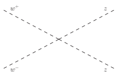
(a)

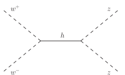
(b)

Figure 1: Tree-level diagrams contributing to the amplitude $w^{+}w^{-}\to zz$, $i\mathcal{M}_{\rm tree}$

Their respective contributions are

$$i\mathcal{M}_{\rm tree}^{(a)}=i\left(\frac{s}{v^{2}}\right),{\text{ and }}i\mathcal{M}_{\rm tree}^{(b)}=-i\left(\frac{a^{2}s}{v^{2}}\right)\left(\frac{s}{s-M_{H}^{2}}\right).$$ (8)

Combined they give

$$i\mathcal{M}_{\rm tree}=-i\left(\frac{s}{v^{2}}\right)\left(\frac{(a^{2}-1)s+M_{H}^{2}}{s-M_{H}^{2}}\right),$$ (9)

which obviously reduces to the same value as the linear case for the SM ($a=1$). Note that in the following the assumption that $p_{i}^{2}=0$ is already made when presenting the amplitude. This expression shows clearly the $\sim s^{2}$ growth of the tree-level amplitude as $s\gg M_{H}^{2}$ if $a\neq 1$ signaling the breakdown of unitarity already at tree-level when one moves away from the SM.

IV One-loop level calculation of $w^{+}w^{-}\to zz$

In the following, the classification of diagrams roughly follows the conventions given in ref. DW , but of course the calculation is completely different as the non-linear realization is used in the present paper and additional topologies of the diagrams do appear. Single diagram includes contributions from internal $h$, $w^{\pm}$, and $z$ loops. We labelled by $(a)$ the subdiagrams for the $h$ loops and by $(b)$ the combined ones for $w^{\pm}$ and $z$ loops.

Here, we will present the radiative corrections to the process grouped in several classes. There are the Higgs self-energy corrections to the diagram in Fig.2 and the vertex corrections in Fig.3. Then we have some irreducible diagrams that following DW we classify as bubbles (in Fig.4), triangles (in Fig.5) and boxes (in Fig.6). In addition we have two new type of diagrams that appear only in the non-linear realization and thus have no counterpart in ref. DW . We have called them five-field (in Fig.7) and six-field (in Fig.8) diagrams, respectively.

IV.1 Higgs self-energy corrections

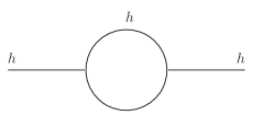
(a)

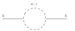
(b)

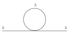
(c)

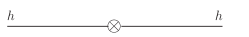
(d)

Figure 2: Radiative corrections to the Higgs two-point function

The two-point diagrams given in DW correspond to $-i\Pi(s)$ and are plotted in Fig. 2. Their contribution to the tree-level diagram $w^{+}w^{-}\to h\to zz$ can be parametrized as

$$i\mathcal{M}_{2-pt}=\left(\frac{a}{v}\right)^{2}\frac{(s)^{2}}{(s-M_{H}^{2})^{2}}\left[-i\Pi(s)\right].$$ (10)

and for $d_{3}=d_{4}=1$ we have

$$i\mathcal{M}_{2-pt} = i\left(\frac{1}{4\pi v^{2}}\right)^{2}\left(\frac{3~{}a^{2}M_{H}^{4}}{2}\right)\frac{s^{2}}{\left(s-M_{H}^{2}\right)^{2}}\times$$

$$\Bigg{(}\frac{A_{0}(M_{H}^{2})}{M_{H}^{2}}+3B_{0}(s,M_{H}^{2},M_{H}^{2})+a^{2}\frac{s^{2}}{M_{H}^{4}}B_{0}(s,0,0)\Bigg{)}$$

$$-i\delta{M_{H}^{2}}\left(\frac{a}{v}\right)^{2}\frac{s^{2}}{(s-M_{H}^{2})^{2}}.$$

The scalar functions $A_{0}$ and $B_{0}$ are described in the appendix and both are ultraviolet divergent. Note that the calculation includes the counterterm for $\delta M_{H}^{2}$ (last line).

IV.2 $hw^{+}w^{-}$ and $hzz$ vertex corrections

The three-point diagrams given in DW correspond to the $hww$/$hzz$ vertex correction $i\Gamma_{3}$, which is also related to the one-loop corrections to the Higgs decay width to $ww$/$zz$. The total correction is the same for both the $hww$ and $hzz$ vertices, although the actual set of diagrams is slightly different for each in the non-linear representation, as there is a 4-$w$ coupling but no 4-$z$ coupling. We draw in Fig.3 diagrams for the case of the $hw^{+}w^{-}$ vertex. Replacing appropriately $w$’s by $z$’s lines, we get the diagrams for the $hzz$ vertex. In this case, however, we only have $z$ internal loops in Fig.3(b).

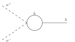
(a)

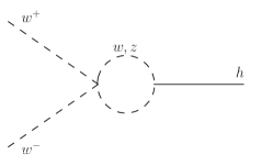
(b)

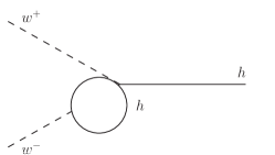
(c)

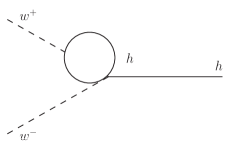
(d)

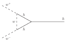
(e)

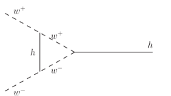
(f)

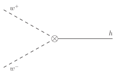
(g)

Figure 3: Three point vertex correction for the $hw^{+}w^{-}$ vertex. A slightly different set of diagrams for the vertex $hzz$ but the result is actually the same.

The rest of the diagrams are the same, however, the total correction can be given as twice the correction to any one vertex to give

$$i\mathcal{M}_{3-pt}=\left(\frac{2a}{v}\right)\frac{s}{(s-M_{H}^{2})}\left[i\Gamma_{3}\right]$$ (12)

We then have (for $d_{3}=d_{4}=1$) the total contribution

$$\!\!\!\!\!\!\!\!i\mathcal{M}_{3-pt} = -i\left(\frac{1}{4\pi v^{2}}\right)^{2}\left(aM_{H}^{4}\right)\left(\frac{s}{s-M_{H}^{2}}\right)\times\Bigg{(}-a(a^{2}-b)\left(\frac{s}{M_{H}^{2}}\right)\Bigg{.}$$

$$+2a\left(\frac{bs-3aM_{H}^{2}}{M_{H}^{2}}\right)\frac{A_{0}(M_{H}^{2})}{M_{H}^{2}}+3\left(\frac{(a^{2}-b)s+2a^{2}M_{H}^{2}}{M_{H}^{2}}\right)B_{0}(s,M_{H}^{2},M_{H}^{2})$$

$$+a\left(\frac{s}{M_{H}^{2}}\right)\left(\frac{(2+a^{2})s-2a^{2}M_{H}^{2}}{M_{H}^{2}}\right)B_{0}(s,0,0)$$

$$+2\left(a^{3}s\right)C_{0}(0,0,s,0,M_{H}^{2},0)-6\left(a^{2}M_{H}^{2}\right)C_{0}(0,0,s,M_{H}^{2},0,M_{H}^{2})\Bigg{)}$$

$$-i(\delta{a})\left(\frac{2as}{v^{2}}\right)\frac{s}{(s-M_{H}^{2})}+i\left(\frac{\delta{v^{2}}}{v^{2}}\right)\left(\frac{a}{v}\right)^{2}\frac{s^{2}}{(s-M_{H}^{2})}$$

Note the inclusion of the counterterms for the parameter $a$ (describing departures from the SM $hww$ and $hzz$ couplings in the non-linear realization) and for the scale $v^{2}$. The (finite) scalar function $C_{0}$ is described in the appendix.

IV.3 Bubble diagrams

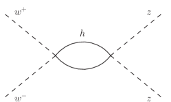
(a)

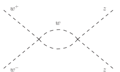
(b)

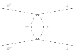
(c)

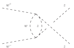
(d)

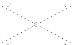
(e)

Figure 4: Bubble diagrams, $i\mathcal{M}_{bubbles}$. Note that we have included the four-point counterterms $\delta a_{4}$ and $\delta a_{5}$ here, but this is simply a choice.

The bubble diagrams are given in Fig. 4 and their contributions for $d_{3}=d_{4}=1$ sum up to

$$i\mathcal{M}_{bubbles} = i\left(\frac{1}{4\pi v^{2}}\right)^{2}\left(\frac{M_{H}^{4}}{2}\right)\times$$

$$\Bigg{(}\left(\frac{-2s^{2}+t^{2}+u^{2}}{9M_{H}^{4}}\right)+\left(\frac{s^{2}}{M_{H}^{4}}\right)\Big{(}b^{2}B_{0}(s,M_{H}^{2},M_{H}^{2})+B_{0}(s,0,0)\Big{)}$$

$$+\left(\frac{t(t-u)}{3M_{H}^{4}}\right)B_{0}(t,0,0)+\left(\frac{u(u-t)}{3M_{H}^{4}}\right)B_{0}(u,0,0)\Bigg{)}$$

$$-i\left(\frac{s}{v^{2}}\right)\left(\frac{\delta_{v^{2}}}{v^{2}}\right)+i\left(\frac{4}{v^{4}}\right)\left((\delta{a_{4}})\left(t^{2}+u^{2}\right)+2(\delta{a_{5}})\left(s^{2}\right)\right)$$

Note the inclusion here of the counterterms for the $O(p^{4})$ coefficients $a_{4}$ and $a_{5}$

IV.4 Triangle diagrams

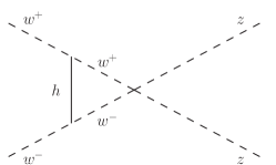
(a)

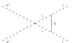
(b)

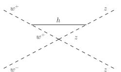
(c)

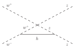
(d)

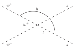
(e)

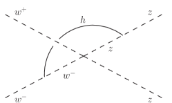
(f)

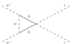
(g)

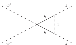
(h)

Figure 5: Triangle diagrams contributing to the irreducible part of the $w^{+}w^{-}\to zz$ amplitude, $i\mathcal{M}_{triangles}$.

The triangle diagrams are given in Fig. 5 and their contributions give (for $d_{3}=d_{4}=1$) the total result

$$\!\!\!\!\!\!\!\!\!i\mathcal{M}_{triangles} = i\left(\frac{1}{4\pi v^{2}}\right)^{2}\left(a^{2}M_{H}^{4}\right)\times$$

$$\!\!\!\!\!\!\Bigg{(}\frac{2s^{2}-t^{2}-u^{2}-18M_{H}^{2}s}{9M_{H}^{4}}-2\left(2\frac{s^{2}}{tu}-(1+b)\frac{s}{M_{H}^{2}}-2\right)\frac{A_{0}(M_{H}^{2})}{M_{H}^{2}}$$

$$\!\!\!\!\!\!-\frac{b\,s}{M_{H}^{2}}\left(\frac{s+2M_{H}^{2}}{M_{H}^{2}}\right)B_{0}(s,M_{H}^{2},M_{H}^{2})+\frac{s}{M_{H}^{2}}\left(\frac{s-2M_{H}^{2}}{M_{H}^{2}}\right)B_{0}(s,0,0)$$

$$\!\!\!\!\!\!+\left(\frac{1}{3}\left(-\frac{t(t-u)}{M_{H}^{4}}+3~{}\frac{t}{M_{H}^{2}}-6~{}\frac{(2s+t)}{t}\right)B_{0}(t,0,0)+(t\Leftrightarrow u)\right)$$

$$\!\!\!\!\!\!+2s\Big{(}b~{}C_{0}(0,0,s,M_{H}^{2},0,M_{H}^{2})-C_{0}(0,0,s,0,M_{H}^{2},0)\Big{)}$$

$$\!\!\!\!\!\!+\left(2\left(-\frac{s}{M_{H}^{2}}-\frac{(2s+t)}{t}\right)M_{H}^{2}~{}C_{0}(0,0,t,0,M_{H}^{2},0)+(t\Leftrightarrow u)\right)\Bigg{)}$$

IV.5 Box diagrams

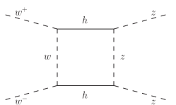
(a)

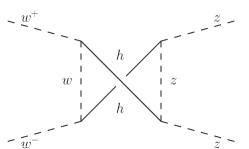
(b)

Figure 6: The box diagrams contributing to the irreducible part of the amplitude, $i\mathcal{M}_{boxes}$.

The box diagrams are depicted in Fig. 6 and their contributions differ only in the exchange of $t\leftrightarrow u$

$$i\mathcal{M}_{boxes} = i\left(\frac{1}{4\pi v^{2}}\right)^{2}\left(a^{4}M_{H}^{4}\right)\times$$

$$\Bigg{(}\frac{1}{18}\left(-\left(\frac{s}{M_{H}^{2}}\right)^{2}+\left(\frac{t}{M_{H}^{2}}\right)^{2}+9\left(\frac{s}{M_{H}^{2}}\right)\right)+\left(-\frac{3}{2}\frac{s}{M_{H}^{2}}+4\frac{t}{u}\right)\frac{A_{0}(M_{H}^{2})}{M_{H}^{2}}$$

$$+\frac{1}{4}\left(\frac{s}{M_{H}^{2}}+2\right)^{2}B_{0}(s,M_{H}^{2},M_{H}^{2})+\left(\frac{1}{6}\frac{t(t-u)}{M_{H}^{4}}-\frac{t}{M_{H}^{2}}-4\frac{t}{u}-1\right)B_{0}(t,0,0)$$

$$-\left(\frac{s}{M_{H}^{2}}+2\right)M_{H}^{2}C_{0}(0,0,s,M_{H}^{2},0,M_{H}^{2})+2\left(\frac{s}{M_{H}^{2}}-\frac{u}{t}\right)M_{H}^{2}C_{0}(0,0,t,0,M_{H}^{2},0)$$

$$+M_{H}^{4}D_{0}(0,0,0,0,s,t,M_{H}^{2},0,M_{H}^{2},0)\Bigg{)}+(t\Leftrightarrow u).$$

The scalar function $D_{0}$ is also described in the appendix.

IV.6 Five-field diagrams

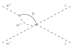
(a)

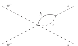
(b)

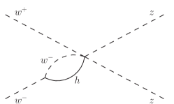
(c)

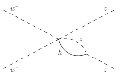
(d)

Figure 7: Five-field diagrams, $i\mathcal{M}_{5F}$. Note that they do not have a counterpart in the linear realization of the SM.

The five-field diagrams do not have a linear calculation counterpart; they are a new topology present in the non-linear description. They are shown in Fig. 7 and they are found by starting from the $wwzz$ four-point vertex and adding a Higgs leg to the central vertex and then connecting it to each of the four external legs. Their inclusion is necessary to make the calculation complete to $\mathcal{O}((M_{H}/v)^{4})$. Summed together they give

$$i\mathcal{M}_{5F} = i\left(\frac{1}{4\pi v^{2}}\right)^{2}\left(a^{2}M_{H}^{4}\right)\left(\frac{s}{M_{H}^{2}}\right)\left(1+2\frac{A_{0}(M_{H}^{2})}{M_{H}^{2}}\right)$$ (17)

IV.7 Six-field diagram

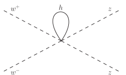
Figure 8: Six-field diagram, $i\mathcal{M}_{6F}$

Finally, there is a single diagram here in which two Higgs legs connect to the central $wwzz$ four-point vertex and then connect to each other to form a single closed loop. As with the five-field case, it is again necessary to ensure the calculation is complete to $\mathcal{O}((M_{H}/v)^{4})$ and similarly has no linear-calculation counterpart. This is given in Fig. 8. It gives

$$i\mathcal{M}_{6F} = i\left(\frac{1}{4\pi v^{2}}\right)^{2}\left(bM_{H}^{4}\right)\left(\frac{s}{M_{H}^{2}}\right)\left(\frac{-A_{0}(M_{H}^{2})}{M_{H}^{2}}\right)$$ (18)

V Wave-function renormalization and tadpoles

V.1 Tadpoles

The one-loop tadpole diagram and counterterm are given in Fig. 9. For $M_{w}=0$, and when assuming the relationship $\lambda=\frac{M_{H}^{2}}{2v^{2}}$ for the renormalized quantities, there is a single contributing diagram to the Higgs tadpole at one-loop: a Higgs loop deriving from a three-Higgs coupling.

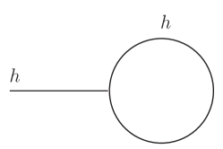
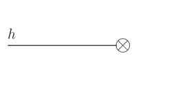
Figure 9: Tadpole diagram and counterterm for the Higgs field.

This gives a value of the tadpole (with external leg removed) of

$$i~{}T = \left(\frac{3d_{3}M_{H}^{2}}{2v}\right)\int\frac{d^{4-\epsilon}k}{(2\pi)^{4-\epsilon}}\frac{1}{\left(k^{2}-M_{H}^{2}\right)}$$

$$= i\left(\frac{1}{4\pi v^{2}}\right)^{2}\left(\frac{3M_{H}^{2}v^{3}}{2}\right)A_{0}\left(M_{H}^{2}\right).$$

From the counterterm lagrangian Eq. (5) the contribution from the tadpole counterterm is

$$i~{}\delta T=-iv\left(\delta{M_{H}^{2}}-2v^{2}\delta{\lambda}-2\lambda\delta{v^{2}}\right).$$ (20)

Therefore, to meet our renormalization condition for vanishing tadpoles at one-loop, we must have

$$\frac{\delta{M_{H}^{2}}}{M_{H}^{2}}-\frac{\delta{\lambda}}{\lambda}-\frac{\delta{v^{2}}}{v^{2}}=-\frac{M_{H}^{2}}{(4\pi v)^{2}}\left(\frac{3}{2}\right)\frac{A_{0}\left(M_{H}^{2}\right)}{M_{H}^{2}}$$ (21)

V.2 Goldstone boson wave-function renormalization

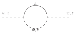
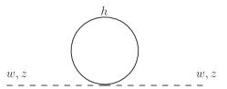
Figure 10: Self-energy for $w$/$z$ fields (contribution to $i\mathcal{M}_{{\text{W}FR}}$)

When all Higgs tadpoles are appropriately canceled, there are only mixed Higgs/Goldstone boson loops, a Higgs loop, and $w/z$ loops (which are zero when the $w/z$ are massless). Any divergences which appear due to the wave-function renormalization of the external fields must be canceled by something in the remainder of this amplitude. We shall see later that this is easily achieved with the renormalization of $v^{2}$, which is also a global factor multiplying the tree-level contribution. In fact from the mere requirement of finiteness of the amplitude after including the one loop diagrams, we can derive only a condition on the combination $2\delta Z_{w}-\delta v^{2}$. Therefore the renormalization condition on the wave function has to be imposed separately and this consists in requesting the unit residue condition on the external legs.

The two-point function for the Goldstone bosons in Fig. 10 gives the following

$$-i\Pi_{w}(q^{2})\equiv-i\Pi_{w}^{(1+2)}(q^{2}) = i\left(\frac{1}{4\pi v^{2}}\right)^{2}(v^{2})\Big{(}\left(a^{2}(3q^{2}-M_{H}^{2})-bq^{2}\right)A_{0}(M_{H}^{2})$$

$$\hskip 78.24507pt+a^{2}(q^{2}-M_{H}^{2})^{2}B_{0}(q^{2},0,M_{H}^{2})\Big{)},$$

which verifies $\Pi_{w}(0)=0$ for all $a$ and $b$, and therefore the Goldstone bosons stay massless, as they should.

The wavefunction renormalization factor is then

$$Z_{w} = 1+\left.\frac{d\Pi_{w}}{dq^{2}}\right|_{q^{2}=0}=1-\left(\frac{1}{4\pi v}\right)^{2}\left((a^{2}-b)A_{0}(M_{H}^{2})+a^{2}\frac{M_{H}^{2}}{2}\right)$$ (23)

In the SM case, this is finite and matches the value given by ref. gupta

$$Z_{w}^{\rm SM} = \left(1-\left(\frac{1}{4\pi v}\right)^{2}\left(\frac{M_{H}^{2}}{2}\right)\right)=\left(1-\frac{\lambda^{2}}{16\pi^{2}}\right)$$ (24)

but in general it is divergent. This divergence is canceled against contributions from $\delta{v^{2}}$ when the corresponding contribution to the one-loop amplitude is placed in the complete calculation. The one-loop contribution to the amplitude $w^{+}w^{-}\to zz$ from wave-function renormalization is

$$i\mathcal{M}_{\rm WFR}=i\left(\frac{1}{4\pi v^{2}}\right)^{2}\left(M_{H}^{2}s\right)\left(\frac{(a^{2}-1)s+M_{H}^{2}}{s-M_{H}^{2}}\right)\left(a^{2}+2(a^{2}-b)\frac{A_{0}(M_{H}^{2})}{M_{H}^{2}}\right)$$ (25)

V.3 Higgs boson wave-function renormalization

The contributions to the Higgs two-point function can be derived from Sec. IV.1, while the counterterm contribution is simply

$$-i\Pi_{H}^{(ctr)}(q^{2})=-i\delta{M_{H}^{2}}$$ (26)

This gives

$$-i\Pi_{H}(q^{2}) = i\left(\frac{1}{4\pi v}\right)^{2}\left(\frac{3M_{H}^{4}}{2}\right)\Bigg{(}\frac{d_{4}}{M_{H}^{2}}A_{0}(M_{H}^{2})+3d_{3}^{2}B_{0}(q^{2},M_{H}^{2},M_{H}^{2})$$

$$\hskip 106.69783pt+a^{2}\frac{s^{2}}{M_{H}^{4}}B_{0}(q^{2},0,0)\Bigg{)}-i\delta{M_{H}^{2}}$$

The on-shell condition for the Higgs mass requires

$${\rm Re}\,\Pi_{H}(M_{H}^{2})=0$$ (28)

Independent of this condition and the counterterm, we have the wavefunction renormalization factor of (now setting $d_{3}=d_{4}=1$)

$$Z_{H} = 1+\left.\frac{d\Pi_{H}}{dq^{2}}\right|_{q^{2}=M_{H}^{2}}$$

$$= 1-\left(\frac{1}{4\pi v}\right)^{2}\left(\frac{3M_{H}^{4}}{2}\right)\left(3B_{0}^{\prime}(M_{H}^{2},M_{H}^{2},M_{H}^{2})+a^{2}\left(B_{0}^{\prime}(M_{H}^{2},0,0)+\frac{2}{M_{H}^{2}}B_{0}(M_{H}^{2},0,0)\right)\right)$$

$$= 1+\left(\frac{M_{H}}{4\pi v}\right)^{2}\left(\left(\frac{9}{2}\right)\left(1-\frac{2\sqrt{3}\pi}{9}\right)+a^{2}\left(\frac{3}{2}-B_{0}(M_{H}^{2},0,0)\right)\right)$$

This is divergent in the SM case and only becomes finite for $a=0$. When the one-loop correction to $i\Gamma(h\to w^{+}w^{-})$ is performed and all external wavefunction renormalizations are included (i.e. both $Z_{H}$ and $Z_{w}$), all divergences cancel for arbitrary $a$ and $b$ when using the appropriate values for the counterterms given in Section VI. This is a good check on this value of $Z_{H}$. It should also be noted that the SM value for $Z_{H}$ does not match that given in ref. gupta ; this is a result of the nonlinear nature of the calculation.

The complete, renormalized decay width for the Higgs boson into Goldstone bosons is

$$\Gamma(h\to ww) = \left(\frac{3\lambda M_{H}a}{16\pi}\right)\Bigg{(}a+\left(\frac{\lambda}{\pi^{2}}\right)\Bigg{\{}\left(\frac{1}{16}\right)\Big{(}a\big{(}17+10b-3a(7a-8)$$

$$\hskip 184.9429pt-2~{}\overline{\delta v^{2}}\big{)}-12b\Big{)}$$

$$\hskip 56.9055pt-\left(\frac{\pi}{8}\right)\sqrt{3}\left(1+3a-b\right)+\left(\frac{\pi^{2}}{48}\right)(a^{2})\left(4+a\right)\Bigg{\}}\Bigg{)},$$

for arbitrary $a$ and $b$, where $\overline{\delta v^{2}}$ is a finite renormalization, not fixed by our conditions. For $a=b=1$ and $~{}\overline{\delta v^{2}}=-\frac{1}{2}$ (the value used in refs. DW and gupta ), this reproduces the known SM result

$$\Gamma(h\to ww) = \left(\frac{3\lambda M_{H}}{16\pi}\right)\Bigg{(}1+\left(\frac{\lambda}{\pi^{2}}\right)\Bigg{\{}\frac{19}{16}-\frac{3\sqrt{3}\pi}{8}+\frac{5\pi^{2}}{48}\Bigg{\}}\Bigg{)}$$ (31)

VI Divergences and determination of the counterterms

Here we give the pieces of each individual diagram proportional to $\Delta_{\epsilon}=\left(\frac{2}{\epsilon}\right)-\gamma_{E}+\log 4\pi+\log\frac{\mu^{2}}{M_{H}^{2}}$. We give the results in the case $d_{3}=d_{4}=1$ but it is quite straightforward to restore these factors for each individual diagram if so desired. These factors appear only in the radiative corrections to two- and three-point functions.

$$\mathcal{M}_{2-pt}^{(a)} \sim \left(\frac{1}{4\pi v^{2}}\right)^{2}\Delta_{\epsilon}\left(\frac{9a^{2}M_{H}^{4}s^{2}}{2(s-M_{H}^{2})^{2}}\right)$$ (32)

$$\mathcal{M}_{2-pt}^{(b)} \sim \left(\frac{1}{4\pi v^{2}}\right)^{2}\Delta_{\epsilon}\left(\frac{3a^{4}s^{4}}{2(s-M_{H}^{2})^{2}}\right)$$

$$\mathcal{M}_{2-pt}^{(c)} \sim \left(\frac{1}{4\pi v^{2}}\right)^{2}\Delta_{\epsilon}\left(\frac{3a^{2}M_{H}^{4}s^{2}}{2(s-M_{H}^{2})^{2}}\right)$$

$$\mathcal{M}_{3-pt}^{(a)} \sim \left(\frac{1}{4\pi v^{2}}\right)^{2}\Delta_{\epsilon}\left(\frac{3abM_{H}^{2}s^{2}}{(s-M_{H}^{2})}\right)$$ (33)

$$\mathcal{M}_{3-pt}^{(b)} \sim \left(\frac{1}{4\pi v^{2}}\right)^{2}\Delta_{\epsilon}\left(\frac{-2a^{2}s^{3}}{(s-M_{H}^{2})}\right)$$

$$\mathcal{M}_{3-pt}^{(c)} \sim \left(\frac{1}{4\pi v^{2}}\right)^{2}\Delta_{\epsilon}\left(\frac{-2a^{2}bM_{H}^{2}s^{2}}{(s-M_{H}^{2})}\right)$$

$$\mathcal{M}_{3-pt}^{(d)} \sim \left(\frac{1}{4\pi v^{2}}\right)^{2}\Delta_{\epsilon}\left(\frac{-3a^{3}M_{H}^{2}s^{2}}{(s-M_{H}^{2})}\right)$$

$$\mathcal{M}_{3-pt}^{(e)} \sim \left(\frac{1}{4\pi v^{2}}\right)^{2}\Delta_{\epsilon}\left(\frac{-a^{4}s^{2}\left(s-2M_{H}^{2}\right)}{(s-M_{H}^{2})}\right)$$

$$\mathcal{M}_{bubble}^{(a)} \sim \left(\frac{1}{4\pi v^{2}}\right)^{2}\Delta_{\epsilon}\left(\frac{b^{2}s^{2}}{2}\right)$$ (34)

$$\mathcal{M}_{bubble}^{(b)} \sim \left(\frac{1}{4\pi v^{2}}\right)^{2}\Delta_{\epsilon}\left(\frac{s^{2}}{2}\right)$$

$$\mathcal{M}_{bubble}^{(c)} \sim \left(\frac{1}{4\pi v^{2}}\right)^{2}\Delta_{\epsilon}\left(\frac{t(t-u)}{6}\right)$$

$$\mathcal{M}_{bubble}^{(d)} \sim \left(\frac{1}{4\pi v^{2}}\right)^{2}\Delta_{\epsilon}\left(\frac{u(u-t)}{6}\right)$$

$$\mathcal{M}_{triangle}^{(a)+(b)} \sim \left(\frac{1}{4\pi v^{2}}\right)^{2}\Delta_{\epsilon}\left(\frac{a^{2}s(3s-2M_{H}^{2})}{3}\right)$$ (35)

$$\mathcal{M}_{triangle}^{(c)+(d)} \sim \left(\frac{1}{4\pi v^{2}}\right)^{2}\Delta_{\epsilon}\left(\frac{-a^{2}t((t-u)-M_{H}^{2})}{3}\right)$$

$$\mathcal{M}_{triangle}^{(e)+(f)} \sim \left(\frac{1}{4\pi v^{2}}\right)^{2}\Delta_{\epsilon}\left(\frac{-a^{2}u((u-t)-M_{H}^{2})}{3}\right)$$

$$\mathcal{M}_{triangle}^{(g)+(h)} \sim \left(\frac{1}{4\pi v^{2}}\right)^{2}\Delta_{\epsilon}\left(-a^{2}bs^{2}\right)$$

$$\mathcal{M}_{box}^{(a)+(b)} \sim \left(\frac{1}{4\pi v^{2}}\right)^{2}\Delta_{\epsilon}\left(\frac{a^{4}\left(s^{2}+t^{2}+u^{2}\right)}{3}\right)$$ (36)

$$\mathcal{M}_{5F}^{(a)+(b)+(c)+(d)} \sim \left(\frac{1}{4\pi v^{2}}\right)^{2}\Delta_{\epsilon}\left(2a^{2}M_{H}^{2}s\right)$$ (37)

$$\mathcal{M}_{6F} \sim \left(\frac{1}{4\pi v^{2}}\right)^{2}\Delta_{\epsilon}\left(-bM_{H}^{2}s\right)$$ (38)

$$\mathcal{M}_{WFR} \sim \left(\frac{1}{4\pi v^{2}}\right)^{2}\Delta_{\epsilon}\left(2M_{H}^{2}s\right)(a^{2}-b)\left(\frac{(a^{2}-1)s+M_{H}^{2}}{(s-M_{H}^{2})}\right)$$ (39)

Note that we have included the $w,z$ Goldstone boson wave-function renormalization as a contribution to the one-loop amplitude to be canceled by the counterterms in $\delta{\mathcal{L}}$.

If we ignore the tadpole counterterms, we can collect together all the individual counterterms to give the following

$$\mathcal{M}^{{\text{c}tr}} = \left(\frac{1}{v^{2}}\right)\left(\frac{s}{\left(s-M_{H}^{2}\right)^{2}}\right)\Bigg{(}\frac{\delta{v^{2}}}{v^{2}}\left((a^{2}-1)s^{2}+(2-a^{2})(sM_{H}^{2})-M_{H}^{4}\right)$$

$$\hskip 92.47145pt-\delta{a}\left((2a)(s)(s-M_{H}^{2})\right)-\frac{\delta{M_{H}^{2}}}{M_{H}^{2}}\left((a^{2})(sM_{H}^{2})\right)\Bigg{)}$$

$$\hskip 7.11317pt+\left(\frac{1}{v^{4}}\right)\Bigg{(}4\delta{a_{4}}(t^{2}+u^{2})+8\delta{a_{5}}(s^{2})\Bigg{)}$$

The values of the counterterms needed to cancel the one-loop divergences—and satisfy our renormalization conditions— can be solved for arbitrary $a$ and $b$ to give

$$\frac{\delta{v^{2}}}{v^{2}} = \frac{M_{H}^{2}}{\left(4\pi v\right)^{2}}\left(\Delta_{\epsilon}(-a^{2}+b)+\overline{\delta v^{2}}\right)$$ (41)

$$\frac{\delta{M_{H}^{2}}}{M_{H}^{2}} = \frac{M_{H}^{2}}{\left(4\pi v\right)^{2}}\left(\frac{3}{2}\right)\left(\Delta_{\epsilon}\left(4+a^{2}\right)+7+2a^{2}-\sqrt{3}\pi\right)$$

$$\frac{\delta{\lambda}}{\lambda} = \frac{M_{H}^{2}}{\left(4\pi v\right)^{2}}\left(\frac{1}{2}\right)\left(\Delta_{\epsilon}\left(9+5a^{2}-2b\right)+18+6a^{2}-3\sqrt{3}\pi-2\overline{\delta v^{2}}\right)$$

$$\delta{a} = \frac{M_{H}^{2}}{\left(4\pi v\right)^{2}}\left(\frac{1}{2}\right)\left(\Delta_{\epsilon}(a-1)(a(5a+2)-3b)\right)$$

$$\delta{a_{4}} = \frac{1}{\left(4\pi\right)^{2}}\left(\frac{-1}{12}\right)\left(\Delta_{\epsilon}\left(a^{2}-1\right)^{2}\right)$$

$$\delta{a_{5}} = \frac{1}{\left(4\pi\right)^{2}}\left(\frac{-1}{48}\right)\left(\Delta_{\epsilon}\left(2+5a^{4}-4a^{2}-6a^{2}b+3b^{2}\right)\right)$$

where $\overline{\delta v^{2}}$ is a finite piece, not determined by the renormalization conditions a priori. Note that the counterterm for $b$ cannot determined from this process. As previously indicated it is quite easy to restore the dependence on $d_{3}$ and $d_{4}$ in the divergent part of all diagrams but we will not present the results here.

VI.1 Cross-checks

In the SM case ($a=b=1$), renormalization conditions read as

$$\frac{\delta{v^{2}}}{v^{2}} = \frac{M_{H}^{2}}{\left(4\pi v\right)^{2}}\left(\overline{\delta v^{2}}\right)$$ (42)

$$\frac{\delta{M_{H}^{2}}}{M_{H}^{2}} = \frac{M_{H}^{2}}{\left(4\pi v\right)^{2}}\left(\frac{3}{2}\right)\left(\Delta_{\epsilon}(5)+9-\sqrt{3}\pi\right)$$

$$\frac{\delta{\lambda}}{\lambda} = \frac{M_{H}^{2}}{\left(4\pi v\right)^{2}}\left(\Delta_{\epsilon}(6)+12-\frac{3}{2}\sqrt{3}\pi-\overline{\delta v^{2}}\right)$$

$$\delta{a} = 0$$

$$\delta{a_{4}} = 0$$

$$\delta{a_{5}} = 0$$

The last three terms should be absent in the SM, so this is a good check. In the EChL case ($a=b=0$) we have

$$\frac{\delta{v^{2}}}{v^{2}} = \frac{M_{H}^{2}}{\left(4\pi v\right)^{2}}\left(\overline{\delta v^{2}}\right)$$ (43)

$$\frac{\delta{M_{H}^{2}}}{M_{H}^{2}} = \frac{M_{H}^{2}}{\left(4\pi v\right)^{2}}\left(\frac{3}{2}\right)\left(\Delta_{\epsilon}(4)+7-\sqrt{3}\pi\right)$$

$$\frac{\delta{\lambda}}{\lambda} = \frac{M_{H}^{2}}{\left(4\pi v\right)^{2}}\left(\Delta_{\epsilon}\left(\frac{9}{2}\right)+9-\frac{3}{2}\sqrt{3}\pi-\overline{\delta v^{2}}\right)$$

$$\delta{a} = 0$$

$$\delta{a_{4}} = \frac{1}{\left(4\pi\right)^{2}}\Delta_{\epsilon}\left(\frac{-1}{12}\right)$$

$$\delta{a_{5}} = \frac{1}{\left(4\pi\right)^{2}}\Delta_{\epsilon}\left(\frac{-1}{24}\right)$$

in agreement with already known results ECHL .

It is interesting to note here that while $\delta{M_{H}^{2}}\neq 0$, its contribution to the counterterm amplitude is actually proportional to $a^{2}$ and therefore vanishes when $a\to 0$ (see Eq. VI). Also, the $\delta{\lambda}$ term is only necessary here to remove the tadpole divergence (which is absent from the full amplitude for $a=b=0$), so once again plays no part. Finally, the $\delta{v^{2}}$ term is finite. Therefore only $\delta{a_{4}}$ and $\delta{a_{5}}$ are needed to remove the one-loop divergences from the Goldstone boson scattering amplitudes, which is what one would expect in the EChL approach.

VII Final result and conclusions

Finally, the complete one-loop amplitude $i\mathcal{M}^{loop}(w^{+}w^{-}\to zz)$ (for arbitrary $a$ and $b$ and rendered finite by using the counterterms in Eq. 41) is given by the following

$$i\mathcal{M}^{loop} = i\left(\frac{1}{4\pi v^{2}}\right)^{2}\left(\frac{M_{H}^{2}}{2}\right)^{2}\Bigg{(}\frac{6a^{2}(-6-2a^{2}+\sqrt{3}\pi)M_{H}^{4}}{(s-M_{H}^{2})^{2}}$$

$$\!\!\!-\frac{4a^{2}\left(18+2a(a-3)+5b-3\sqrt{3}\pi-\overline{\delta v^{2}}\right)M_{H}^{2}}{(s-M_{H}^{2})}$$

$$\!\!\!-\frac{2}{9}(a^{2}-1)\left((a^{2}-1)\,\frac{t^{2}+4tu+u^{2}}{M_{H}^{4}}-72a^{2}\,\frac{t^{2}+tu+u^{2}}{tu}\right)$$

$$\!\!\!+4\left(\frac{s}{M_{H}^{2}}\right)\left(2a^{4}-3a^{2}b+b+(a^{2}-1)\overline{\delta v^{2}}\right)+a^{2}\left(6\sqrt{3}\pi-4(9+3a(a-2)+5b-\overline{\delta v^{2}}\,)\right)$$

$$\!\!\!+2\left(\frac{(a^{2}-b)s^{2}+((a^{2}-b)-3a)M_{H}^{2}s-2a^{2}M_{H}^{4}}{M_{H}^{2}(s-M_{H}^{2})}\right)^{2}\overline{B}_{0}(s,M_{H}^{2},M_{H}^{2})$$

$$\!\!\!+2\frac{s\left((a^{2}-1)s+M_{H}^{2}\right)}{M_{H}^{4}}\left(\frac{(a^{2}-1)s^{2}+(6a^{2}+1)M_{H}^{2}s-4a^{2}M_{H}^{4}}{(s-M_{H}^{2})^{2}}\right)\overline{B}_{0}(s,0,0)$$

$$\!\!\!+\Bigg{(}\Bigg{(}\frac{4(a^{2}-1)^{2}}{3}\frac{t^{2}}{M_{H}^{4}}+\frac{2(a^{2}-1)}{3}\frac{((a^{2}-1)s-6a^{2}M_{H}^{2})}{M_{H}^{2}}\frac{t}{M_{H}^{2}}$$

$$\!\!\!\hskip 28.45274pt+4a^{2}\left(1-(a^{2}-1)\left(1+4\frac{u}{t}\right)\right)\Bigg{)}\overline{B}_{0}(t,0,0)+(t\Leftrightarrow u)\Bigg{)}$$

$$\!\!\!-8a^{2}\frac{(a^{2}-b)s^{2}+((a^{2}-b)-3a)M_{H}^{2}s-2a^{2}M_{H}^{4}}{(s-M_{H}^{2})}\,C_{0}(0,0,s,M_{H}^{2},0,M_{H}^{2})$$

$$\!\!\!+8a^{2}\frac{s}{(s-M_{H}^{2})}\left((a^{2}-1)s+M_{H}^{2}\right)C_{0}(0,0,s,0,M_{H}^{2},0)$$

$$+\Bigg{(}8a^{2}\left((a^{2}-1)s+M_{H}^{2}\left(1-2(a^{2}-1)\,\frac{u}{t}\right)\right)C_{0}(0,0,t,0,M_{H}^{2},0)+(t\Leftrightarrow u)\Bigg{)}$$

$$\!\!\!+\Bigg{(}4a^{2}M_{H}^{4}D_{0}(0,0,0,0,s,t,M_{H}^{2},0,M_{H}^{2},0)+(t\Leftrightarrow u)\Bigg{)}\Bigg{)}$$

Here the functions $\bar{A_{0}}$ and $\bar{B_{0}}$ are the corresponding scalar integral functions with the divergences removed (see appendix). The amplitude as written above has been grouped by scalar loop integrals. In the SM limit ($a=b=1$), this simplifies quite a bit

$$i\mathcal{M}^{loop}_{SM} = i\left(\frac{1}{4\pi v^{2}}\right)^{2}\left(\frac{M_{H}^{2}}{2}\right)^{2}\Bigg{(}$$

$$+\frac{M_{H}^{4}}{(s-M_{H}^{2})^{2}}\left(-48+6\sqrt{3}\pi+18\overline{B}_{0}(s,M_{H}^{2},M_{H}^{2})+6\overline{B}_{0}(s,0,0)\right)$$

$$+\frac{M_{H}^{2}}{(s-M_{H}^{2})}\Big{(}-76+12\sqrt{3}\pi+4\overline{\delta v^{2}}+12\overline{B}_{0}(s,M_{H}^{2},M_{H}^{2})+20\overline{B}_{0}(s,0,0)$$

$$\hskip 71.13188pt+(8M_{H}^{2})\Big{(}3C_{0}(0,0,s,M_{H}^{2},0,M_{H}^{2})+C_{0}(0,0,s,0,M_{H}^{2},0)\Big{)}\Big{)}$$

$$+\Big{(}2\overline{B}_{0}(s,M_{H}^{2},M_{H}^{2})+14\overline{B}_{0}(s,0,0)+4\overline{B}_{0}(t,0,0)+4\overline{B}_{0}(u,0,0)\Big{)}$$

$$+(8M_{H}^{2})\Big{(}C_{0}(0,0,s,M_{H}^{2},0,M_{H}^{2})+C_{0}(0,0,s,0,M_{H}^{2},0)$$

$$\hskip 42.67912pt+C_{0}(0,0,t,0,M_{H}^{2},0)+C_{0}(0,0,u,0,M_{H}^{2},0)\Big{)}$$

$$+(4M_{H}^{4})\Big{(}D_{0}(0,0,0,0,s,t,M_{H}^{2},0,M_{H}^{2},0)+D_{0}(0,0,0,0,s,u,M_{H}^{2},0,M_{H}^{2},0)\Big{)}$$

$$-2\left(22-3\sqrt{3}\pi-2\overline{\delta v^{2}}\right)\Bigg{)}$$

Eqs. 41 and VII contain our main results. We have seen how the departures from the SM can be taken consistently into account in an effective-Lagrangian philosophy also at the one-loop level and the suitable counterterms included to render the amplitude finite. We note that if $a$ and $b$ are set to their SM values, the coefficients accompanying the $O(p^{4})$ operators are finite and do not run, while this is not the case as soon as one departs from the SM. After cancellation of the divergent part of the loop (say in the $\overline{MS}$ scheme), a finite logarithmic part remains. For instance in the case of the effective coefficients $a_{4}$ and $a_{5}$, and appealing to naturality arguments, their characteristic size would be

$$\delta{a_{4}} = \frac{1}{\left(4\pi\right)^{2}}\left(\frac{-1}{12}\right)\left(a^{2}-1\right)^{2}\log\frac{f^{2}}{v^{2}}$$ (46)

$$\delta{a_{5}} = \frac{1}{\left(4\pi\right)^{2}}\left(\frac{-1}{48}\right)\left(2+5a^{4}-4a^{2}-6a^{2}b+3b^{2}\right)\log\frac{f^{2}}{v^{2}}$$

$f$ being the compositeness scale.

In the present study we have restricted ourselves to the case where the triple and quartic Higgs coupling take the same values as in the SM, but relaxing this hypothesis is straightforward. The dependence of the divergent parts on $d_{3}$ and $d_{4}$ can be easily determined as they simply contribute as overall factors to vertex and self-energy corrections. None of those diagrams behave as $\sim s^{2}$ (or as $t^{2}$ or $u^{2}$) for large values of $s$ and they therefore do not contribute to $\delta a_{4}$ and $\delta a_{5}$ that are totally independent of $d_{3}$ and $d_{4}$.

It would be interesting to extend the present study to other low energy constants of the effective theory parametrizing the EWSBS. In particular $a_{1}$ and $a_{2}$ correspond to operators that contribute to the triple gauge boson vertex that has been recently measured for the first time at the LHC TGC . The renormalization of $d_{3}$ and $d_{4}$ would eventually be of interest too, but their relevance for comparison with experiment is still well ahead.

We have also presented a full one-loop calculation using the Equivalence Theorem approximation (and taking the masses of the Goldstone bosons to vanish, i.e. in the ’t Hooft-Landau gauge) of the $W_{L}W_{L}\to Z_{L}Z_{L}$ in the general case with generic couplings of the Higgs to the electroweak gauge bosons. This calculation should be quite useful in precise comparisons of measurements of the four gauge boson coupling (not yet measured at the LHC) to theoretical predictions. Its knowledge is also very relevant in connection with unitarity analysis such as the one done in EY and the prediction of new resonances originating from the EWSBS. As emphasized in the introduction, the search for such resonances has to go hand-in-hand with accurate measurements of the four gauge boson couplings. Almost any deviation of these coefficients from their SM values would lead to unitarity violations at high energies and thus require additional resonances to restore it. In a forthcoming publication we will study in detail the issue of unitarity and extend the results of EY to the case where the tree-level $O(p^{2})$ parameters $a$ and $b$ depart from their SM values. Both the determination of the counterterms and the full calculation of the real part of the scattering amplitude derived in this preparatory paper are necessary ingredients for such an analysis.

In conclusion, we have successfully provided a one-loop theory of Goldstone boson scattering in the context of an extended EWSBS where the Higgs is allowed to have arbitrary couplings. The coefficients $a$ and $b$ describing the coupling of the Higgs to the $W$ and $Z$ gauge bosons are currently of great interest to SM fits but their treatment so far has only been of tree-level studies. If $a$ and $b$ are not exactly equal to one some $O(p^{4})$ operators with running coefficients are required for a consistent treatment at one loop. Their running has been determined in this work. The results smoothly connect to the SM and are, we believe, completely general.

Appendix

Here we define the independent scalar integrals entering our expressions

$$A_{0}(m^{2}_{0}) = {\cal N}\int d^{d}k\dfrac{1}{k^{2}-m^{2}_{0}}=m^{2}_{0}\left(\Delta_{\epsilon}+1\right)$$ (47)

$$B_{0}(p_{1}^{2},m^{2}_{0},m^{2}_{1}) = {\cal N}\int d^{d}k\dfrac{1}{k^{2}-m^{2}_{0}}\dfrac{1}{(k+p_{1})^{2}-m^{2}_{1}}$$

$$C_{0}(p_{1}^{2},p_{2}^{2},p_{12}^{2},m^{2}_{0},.,m^{2}_{3}) = {\cal N}\int d^{d}k\dfrac{1}{k^{2}-m^{2}_{0}}\dfrac{1}{(k+p_{1})^{2}-m^{2}_{1}}\dfrac{1}{(k+p_{12})^{2}-m^{2}_{2}}$$

$$D_{0}(p_{1}^{2},p_{2}^{2},p_{3}^{2},p_{13}^{2},p_{12}^{2},p_{23}^{2},m^{2}_{0},.,m^{2}_{3})=$$ (48)

$${\cal N}\int d^{d}k\dfrac{1}{k^{2}-m^{2}_{0}}\dfrac{1}{(k+p_{1})^{2}-m^{2}_{1}}\dfrac{1}{(k+p_{12})^{2}-m^{2}_{2}}\dfrac{1}{(k+p_{13})^{2}-m^{2}_{3}}$$ (49)

where ${\cal N}=(2\pi\mu)^{4-d}/(i\pi^{2})$ and $p_{ij}=\sum_{h=i}^{j}p_{h}$. We note that of the scalar loop integrals ($A_{0}$, $B_{0}$, $C_{0}$, and $D_{0}$) in our solution only $A_{0}$ and $B_{0}$ contain divergences. We will therefore define the functions $\bar{A_{0}}$ and $\bar{B_{0}}$ as the corresponding scalar integral functions with the divergences removed

$$A_{0}(a) = a\Delta_{\epsilon}+\bar{A_{0}}(a)$$ (50)

$$B_{0}(a,b,c) = \Delta_{\epsilon}+\bar{B_{0}}(a,b,c)$$

Note that this differs slightly from the $\Delta_{\epsilon}=(\frac{2}{\epsilon}-\gamma_{E}+\log 4\pi)$ used in the literature on the scalar loop integrals. However, this has the benefit that all factors of $\log\frac{\mu^{2}}{M_{H}^{2}}$ are currently in the counterterms and that $\bar{A_{0}}(M_{H}^{2})=M_{H}^{2}$. For situations in which it is better to have $\log\frac{\mu^{2}}{M_{H}^{2}}$ explicitly in the amplitude (for instance in the limit $M_{H}^{2}\to\infty$), this can be achieved by replacing each counterterm in Eq. VI with $\mathcal{C}\log\frac{\mu^{2}}{M_{H}^{2}}$ —where $\mathcal{C}$ is the coefficient of the divergent part of the corresponding counterterm— and then adding it to the amplitude.

References

- (1) D. Espriu and B. Yencho, Phys. Rev. D 87, 055017 (2013).
- (2) G. Aad et al. [The ATLAS collaboration], Phys. Lett. B 716 (2012) 1.
- (3) S.Chatrchyan et al. [The CMS collaboration], Phys. Lett. B 716 (2012) 30.
- (4) A. Dobado, D. Espriu and M.J. Herrero, Phys.Lett. B255 (1991) 405; D. Espriu and M.J. Herrero, Nucl.Phys. B373 (1992) 117; M.J. Herrero and E. Ruiz-Morales, Nucl.Phys. B418 (1994) 431; Nucl. Phys. B 437 (1995) 319; D. Espriu and J. Matias, Phys.Lett. B341 (1995) 332; A. Dobado, M.J. Herrero, J.R. Peláez and E. Ruiz-Morales, Phys. Rev. D 62 (2000) 05501; R. Foadi, M. Jarvinen and F. Sannino, Phys. Rev. D 79, 035010 (2009) [arXiv:0811.3719 [hep-ph]].
- (5) G. F. Giudice, C. Grojean, A. Pomarol and R. Rattazzi, JHEP 0706, 045 (2007) [hep-ph/0703164]; R. Contino, M. Ghezzi, C. Grojean, M. Muhlleitner and M. Spira, arXiv:1303.3876 [hep-ph]; R. Alonso, M. B. Gavela, L. Merlo, S. Rigolin and J. Yepes, Phys. Lett. B 722, 330 (2013) [arXiv:1212.3305 [hep-ph]].
- (6) G. Belanger, B. Dumont, U. Ellwanger, J. F. Gunion and S. Kraml, arXiv:1306.2941 [hep-ph]; T. Corbett, O. J. P. Eboli, J. Gonzalez-Fraile and M. C. Gonzalez-Garcia, Phys. Rev. D 86, 075013 (2012) [arXiv:1207.1344 [hep-ph]]; arXiv:1306.0006 [hep-ph]; J. Ellis and T. You, arXiv:1303.3879 [hep-ph]; P. P. Giardino, K. Kannike, I. Masina, M. Raidal and A. Strumia, arXiv:1303.3570 [hep-ph]; A. Falkowski, F. Riva and A. Urbano, arXiv:1303.1812 [hep-ph]; T. Alanne, S. Di Chiara and K. Tuominen, arXiv:1303.3615 [hep-ph].
- (7) O. Cheyette and M.K. Gaillard, Phys. Lett. B 197 (1987) 205; A. Dobado, M.J. Herrero and T.N. Truong Phys.Lett. B235 (1990) 129; W. Dicus and W.W. Repko, Phys. Rev. D 42 (1990) 3660; Phys. Rev. D 44 (1991) 3473; Phys. Rev. D 47 (1993) 415; J.R. Peláez, Phys. Rev. D 55 (1997) 4193.
- (8) J.M. Cornwall, D.N. Levin and G.Tiktopoulos, Phys. Rev. D10 (1974) 1145 ; B.W. Lee, C. Quigg and H. Thacker, Phys. Rev. D16 (1977) 1519; G.J. Gounaris, R. Kogerler and H. Neufeld, Phys. Rev. D34 (1986) 3257; M.S. Chanowitz and M.K. Gaillard, Nucl. Phys. B261 (1985) 379; A. Dobado and J.R. Peláez, Nucl.Phys. B425 (1994) 110; Phys. Lett. B329 (1994) 469; C. Grosse-Knetter and I.Kuss, Z.Phys. C66 (1995) 95; H.J.He,Y.P.Kuang and X.Li, Phys. Lett. B329 (1994) 278.
- (9) D. Espriu and J. Matias, Phys. Rev. D 52 (1995) 6530.
- (10) T.N. Truong, Phys. Rev. Lett. 61 (1988) 2526; A. Dobado, M.J. Herrero and T.N. Truong, Phys.Lett. B235 (1990) 134; A. Dobado and J.R. Peláez, Phys. Rev. D 47 (1993) 4883; Phys. Rev. D 56 (1997) 3057; J.A. Oller, E. Oset and J.R. Peláez, Phys. Rev. Lett. 80 (1998) 3452; Phys. Rev. D 59 (1999) 0740001; 60 (1999) 099906; F. Guerrero and J.A. Oller, Nucl. Phys. B 537 (1999) 459; A. Dobado and J.R. Peláez, Phys. Rev D 65 (2002) 077502.
- (11) A. Denner, S. Dittmaier and T. Hahn, Phys.Rev. D56 (1997) 117; A. Denner and T. Hahn, Nucl.Phys. B525 (1998) 27.
- (12) S. Dawson and S. Willenbrock, Phys. Rev. D 40 (1989) 2880.
- (13) S. N. Gupta, J. M. Johnson and W. W. Repko, Phys. Rev. D 48, 2083 (1993).
- (14) T. Corbett, O. J. P. Eboli, J. Gonzalez-Fraile and M. C. Gonzalez-Garcia, arXiv:1304.1151 [hep-ph]; G. Aad et al. [ATLAS Collaboration], Phys. Rev. D 87, 112001 (2013) [arXiv:1210.2979 [hep-ex]]; Eur. Phys. J. C 72, 2173 (2012) [arXiv:1208.1390 [hep-ex]]; G. Aad et al. [ATLAS Collaboration], Phys. Rev. D 87, 112003 (2013) [arXiv:1302.1283 [hep-ex]]; S. Chatrchyan et al. [CMS Collaboration], Eur. Phys. J. C 73, 2283 (2013) [arXiv:1210.7544 [hep-ex]].