Investigation of the $D^{\ast}_{s}D_{s}\eta^{(\prime)}$ and $B^{\ast}_{s}B_{s}\eta^{(\prime)}$ vertices via QCD sum rules

Abstract

The strong coupling constants among mesons are very important quantities as they can provide useful information on the nature of strong interaction among hadrons as well as the QCD vacuum. In this article, we investigate the strong vertices of the $D^{\ast}_{s}D_{s}\eta^{(\prime)}$ and $B^{\ast}_{s}B_{s}\eta^{(\prime)}$ in the framework of the QCD sum rule approach choosing the $\eta$ or $D_{s}(B_{s})$ meson as an off-shell state. We obtain the results $g_{D_{s}^{*}D_{s}\eta}=(1.46\pm 0.30)GeV^{-1}$, $g_{D_{s}^{*}D_{s}\eta^{\prime}}=(0.74\pm 0.16)GeV^{-1}$, $g_{B_{s}^{*}B_{s}\eta}=(5.29\pm 1.06)GeV^{-1}$ and $g_{B_{s}^{*}B_{s}\eta^{\prime}}=(2.29\pm 0.48)GeV^{-1}$ for the strong coupling constants under consideration, which can be checked in future experiments.

I Introduction

In the last few years, both the experimental and theoretical studies on the properties of heavy mesons have received considerable attention. With the growing data collected by many experimental groups, the investigations of the spectroscopy as well as the electromagnetic, weak and strong decay properties of the charmed(bottom)–strange mesons have become more interesting [1-6]. Hence, theoretical determination of various characteristics related to these mesons, such as transition form factors and coupling constants, become very important for interpretation of the experimental results.

In the low energy regime of QCD, the large value of the strong coupling constant does not allow us to use the perturbative theories. Hence, some non-perturbative methods are needed to investigate the hadronic properties. The QCD sum rules approach shifman is one of the effective tools in this respect since it is based on QCD Lagrangian and do not include any model-dependent parameter. According to the QCD sum rules method, the strong coupling constants among three mesons are calculated by using three point correlation functions. In the present work, we apply this technique to investigate the strong coupling constants among $D_{s}^{*}[B_{s}^{*}]$ and $D_{s}[B_{s}]$ mesons with light pseudoscalar $\eta$ and $\eta^{\prime}$ mesons. For some applications of this method to hadron physics, specially the strong decays see bracco ; wang ; bracco2 ; bracco3 ; bracco4 ; bracco5 ; bracco6 ; bracco7 ; wang2 ; bracco8 ; wang3 ; maris ; gamiz ; rosner ; lucha ; bracco9 ; bracco10 ; hollanda ; azizi ; cui .

Taking into account only the strong force, the basic SU(3) flavor symmetry for the three light quarks predicts the singlet $\eta_{1}$ and octet $\eta_{8}$ particles:

$$|\eta_{1}\rangle=\frac{1}{\sqrt{3}}|u\bar{u}+d\bar{d}+s\bar{s}\rangle,\mbox{ }|\eta_{8}\rangle=\frac{1}{\sqrt{6}}|u\bar{u}+d\bar{d}-2s\bar{s}\rangle.$$ (1)

On the other hand, due to the electromagnetic and weak interactions, a mixing of these singlet and octet states occurs because of the transformation of one quark flavor into another. The physical $\eta$ and $\eta^{\prime}$ states are the linear combinations of these SU(3) singlet and octet states:

$$\left(\begin{array}[]{c}\eta\\ \eta^{\prime}\end{array}\right)=\left(\begin{array}[]{cc}\cos\theta&-\sin\theta\\ \sin\theta&\cos\theta\end{array}\right)\left(\begin{array}[]{c}\eta_{8}\\ \eta_{1}\end{array}\right),$$ (2)

were $\theta$ is the mixing angle of the singlet-octet representation SVDonskov . Even though the QCD sum rule is a powerful method for investigation of the non-perturbative nature of particles, the predictions of this approach have considerable uncertainties due to the uncertainties implemented by the quark-hadron duality, determination of the working regions for the Borel mass parameters, quark masses, radiative corrections, etc. Hence the relatively small effect of the mixing angle allows us to neglect the mixing of the singlet and octet states when QCD sum rules method is used. In other words, the $\eta$ and $\eta^{\prime}$ can be taken as pure octet and singlet states, respectively.

The outline of this article is as follows: in section II, we calculate the three point correlation functions for $D^{\ast}_{s}D_{s}\eta^{(\prime)}$ and $B^{\ast}_{s}B_{s}\eta^{(\prime)}$ vertices, when $D_{s}[B_{s}]$ or $\eta[\eta^{\prime}]$ meson is off-shell. Taking into account the quark and mixed condensate diagrams we obtain QCD sum rules for the strong coupling form factors of each vertex. In section III, we present our numerical calculations of the obtained sum rules and calculate the values of the strong coupling constants for each vertex.

II QCD Sum Rules for strong Coupling form factors

In this section, we obtain QCD sum rules for strong coupling form factors associated with the $D^{\ast}_{s}D_{s}\eta[D^{\ast}_{s}D_{s}\eta^{\prime}]$ and $B^{\ast}_{s}B_{s}\eta[B^{\ast}_{s}B_{s}\eta^{\prime}]$ vertices by considering the following three-point correlation functions:

$$\Pi_{\mu}^{D_{s}[B_{s}]}(p^{\prime},q)=i^{2}\int d^{4}x~{}d^{4}y~{}e^{ip^{\prime}\cdot x}~{}e^{iq\cdot y}{\langle}0|{\cal T}\left(J^{\eta}(x)~{}J^{D_{s}[B_{s}]}(y)~{}J^{D_{s}^{\ast}[B_{s}^{\ast}]{\dagger}}_{\mu}(0)\right)|0{\rangle},$$

$$\Pi_{\mu}^{D_{s}[B_{s}]}(p^{\prime},q)=i^{2}\int d^{4}x~{}d^{4}y~{}e^{ip^{\prime}\cdot x}~{}e^{iq\cdot y}{\langle}0|{\cal T}\left(J^{\eta^{\prime}}(x)~{}J^{D_{s}[B_{s}]}(y)~{}J^{D_{s}^{\ast}[B_{s}^{\ast}]{\dagger}}_{\mu}(0)\right)|0{\rangle}$$ (3)

for the case of $D_{s}[B_{s}]$ off-shell. Similarly we consider the correlation functions for the off-shell $\eta$ and $\eta^{\prime}$ cases. In Eq. (II) ${\cal T}$ is the time ordering operator and $q=p-p^{\prime}$ is transferred momentum. The interpolating currents of the participating mesons can be written in terms of the quark fields as

$$J^{\eta}(x) = \frac{1}{\sqrt{6}}\Big{[}\overline{u}(x)\gamma_{5}u(x)+\overline{d}(x)\gamma_{5}d(x)-2\overline{s}(x)\gamma_{5}s(x)\Big{]},$$

$$J^{\eta^{\prime}}(x) = \frac{1}{\sqrt{3}}\Big{[}\overline{u}(x)\gamma_{5}u(x)+\overline{d}(x)\gamma_{5}d(x)+\overline{s}(x)\gamma_{5}s(x)\Big{]},$$ (4)

$$J^{D_{s}[B_{s}]}(x)=\overline{s}(x)\gamma_{5}c[b](x),$$

$$J^{D_{s}^{\ast}[B_{s}^{\ast}]}_{\mu}(x)=\overline{s}(x)\gamma_{\mu}c[b](x).$$

The above mentioned correlation functions can be calculated in two different ways. From phenomenological or physical side, they are obtained in terms of hadronic parameters. From theoretical or QCD side, they are evaluated in terms of quark’s and gluon’s degrees of freedom by the help of the operator product expansion (OPE) in deep Euclidean region. After equating the coefficients of individual structures from both sides of the same correlation functions, the sum rules for the strong coupling form factors are obtained. Finally we apply Double Borel transformation with respect to the variables, $p^{2}$ and $p^{\prime 2}$ to suppress the contribution of the higher states and continuum. According to the general philosophy of the method, we also use the quark-hadron duality assumption.

First, we calculate the physical sides of the correlation functions in Eq. (II) for the off-shell $D_{s}[B_{s}]$ state. They are obtained by saturating them with the complete sets of appropriate $D_{s}$, $D_{s}^{\ast}$ and $\eta^{(\prime)}$ states with the same quantum numbers as the corresponding mesonic interpolating currents. After performing the four-integrals over $x$ and $y$, for both $\eta$ and $\eta^{\prime}$ cases in a compact form, we get

$$\Pi_{\mu}^{D_{s}[B_{s}]}(p^{\prime},q)$$ (5)

$$= \frac{{\langle}0|J^{\eta^{(\prime)}}|\eta^{(\prime)}(p^{\prime}){\rangle}{\langle}0|J^{D_{s}[B_{s}]}|D_{s}[B_{s}](q){\rangle}{\langle}\eta^{(\prime)}(p^{\prime})D_{s}[B_{s}](q)|D_{s}^{\ast}[B_{s}^{\ast}](p,\epsilon){\rangle}{\langle}D_{s}^{\ast}[B_{s}^{\ast}](p,\epsilon)|J^{D_{s}^{\ast}[B_{s}^{\ast}]}_{\mu}|0{\rangle}}{(q^{2}-m_{D_{s}[B_{s}]}^{2})(p^{2}-m_{D_{s}^{\ast}[B_{s}^{\ast}]}^{2})({p^{\prime}}^{2}-m_{\eta^{(\prime)}}^{2})}$$

$$+ ...,$$

where …. stands for the contributions of the higher states and continuum. To proceed we need to define the following matrix elements in terms of hadronic parameters:

$${\langle}0|J^{\eta^{(\prime)}}|\eta^{(\prime)}(p^{\prime}){\rangle} = \frac{m_{\eta^{(\prime)}}^{2}f_{\eta^{(\prime)}}}{2m_{s}},$$

$${\langle}0|J^{D_{s}[B_{s}]}|D_{s}[B_{s}](q){\rangle} = \frac{m_{D_{s}[B_{s}]}^{2}~{}f_{D_{s}[B_{s}]}}{m_{c(b)}+m_{s}},$$

$${\langle}D_{s}^{\ast}[B_{s}^{\ast}](p,\epsilon)|J^{D_{s}^{\ast}[B_{s}^{\ast}]}_{\mu}|0{\rangle} = m_{D_{s}^{\ast}[B_{s}^{\ast}]}f_{D_{s}^{\ast}[B_{s}^{\ast}]}{\epsilon^{\ast}}_{\mu},$$

$${\langle}\eta^{(\prime)}(p^{\prime})D_{s}[B_{s}](q)|D^{\ast}_{s}[B^{\ast}_{s}](p,\epsilon){\rangle} = g_{D^{\ast}_{s}D_{s}\eta^{(\prime)}[B^{\ast}_{s}B_{s}\eta^{(\prime)}]}^{D_{s}[B_{s}]}(p^{\prime}-q)\cdot\epsilon,$$ (6)

where $g_{D^{\ast}_{s}D_{s}\eta^{(\prime)}[B^{\ast}_{s}B_{s}\eta^{(\prime)}]}^{D_{s}[B_{s}]}$ is the strong coupling form factor; and $f_{D_{s}^{\ast}[B_{s}^{\ast}]}$, $f_{D_{s}[B_{s}]}$ and $f_{\eta^{(\prime)}}$ are leptonic decay constants of the $D_{s}^{\ast}[B_{s}^{\ast}]$, $D_{s}[B_{s}]$ and $\eta^{(\prime)}$ mesons, respectively. Using Eq. (II) in Eq. (5) and summing over polarization vectors, we obtain the physical side as

$$\Pi_{\mu}^{D_{s}[B_{s}]}(p^{\prime},q) = g^{D_{s}[B_{s}]}_{D^{\ast}_{s}D_{s}\eta^{(\prime)}[B^{\ast}_{s}B_{s}\eta^{(\prime)}]}\frac{f_{D_{s}^{\ast}[B_{s}^{\ast}]}m_{D_{s}^{\ast}[B_{s}^{\ast}]}f_{\eta^{(\prime)}}m_{\eta^{(\prime)}}^{2}f_{D_{s}[B_{s}]}m_{D_{s}[B_{s}]}^{2}}{(q^{2}-m_{D_{s}[B_{s}]}^{2})(p^{\prime^{2}}-m_{\eta^{(\prime)}}^{2})(p^{2}-m_{D_{s}^{\ast}(B_{s}^{\ast})}^{2})2m_{s}(m_{c(b)}+m_{s})}$$

$$\times\Big{[}\Big{(}1+\frac{m_{\eta^{(\prime)}}^{2}-q^{2}}{m_{D_{s}^{\ast}[B_{s}^{\ast}]}^{2}}\Big{)}p_{\mu}-2p^{\prime}_{\mu}\Big{]}+....,$$

where we will choose the structure $p_{\mu}$ to calculate the corresponding strong coupling form factor. From a similar manner, one can obtain the final expression of the physical side of the correlation function for an $\eta^{(\prime)}$ off-shell.

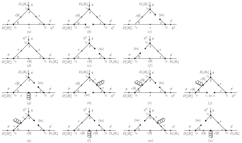
Figure 1: Diagrams considered in the calculations.

From the QCD or theoretical side, the aforesaid correlation functions are calculated in deep Euclidean space, where $p^{2}\rightarrow-\infty$ and ${p^{\prime}}^{2}\rightarrow-\infty$ by the help of OPE. To obtain the QCD representation, as an example for the $D_{s}[B_{s}]$ off-shel case, we separate the correlation function into perturbative and non-perturbative parts and keep only the structure which we use to extract the sum rules

$$\Pi^{D_{s}[B_{s}]}_{\mu}(p^{\prime},q) = \left(\Pi_{per}+\Pi_{nonper}\right)p_{\mu}+...,$$ (8)

where the perturbative part can be expressed in terms of a double dispersion integral of the form

$$\Pi_{per} = -\frac{1}{4\pi^{2}}\int ds\int ds^{\prime}\frac{\rho(s,s^{\prime},q^{2})}{(s-p^{2})(s^{\prime}-{p^{\prime}}^{2})}+\mbox{subtraction terms},$$ (9)

with $\rho(s,s^{\prime},q^{2})$ being the corresponding spectral density. Our main task in the following is to calculate this spectral density. For this aim, we consider the bare loop diagrams (a) and (d) in Fig. 1 for $D_{s}[B_{s}]$ as off-shell state. We calculate these diagrams via Cutkosky rules, as a result of which we get

$$\rho^{D_{s}[B_{s}]}(s,s^{\prime},q^{2}) = -\frac{N_{c}}{\lambda^{3/2}(s,s^{\prime},q^{2})}\left\{m_{c[b]}^{2}s^{\prime}(q^{2}-s+s^{\prime})-m_{s}^{2}s^{\prime}(q^{2}-s+s^{\prime})+q^{2}s^{\prime}(-q^{2}+s+s^{\prime})\right\}.$$

Similarly, for the case of $\eta^{(\prime)}$ off-shel one gets

$$\rho^{\eta^{(\prime)}}(s,s^{\prime},q^{2}) = \frac{N_{c}}{\lambda^{3/2}(s,s^{\prime},q^{2})}\left\{m_{s}^{2}\Big{(}q^{4}-2q^{2}s+(s-s^{\prime})^{2}\Big{)}-m_{c[b]}m_{s}\Big{(}q^{4}+(s-s^{\prime})^{2}-2q^{2}(s+s^{\prime})\Big{)}\right.$$ (11)

$$- \left.2m_{c[b]}^{2}q^{2}s^{\prime}(s+s^{\prime}-q^{2})\right\},$$

where $\lambda(a,b,c)=a^{2}+b^{2}+c^{2}-2ac-2bc-2ab$ and $N_{c}=3$ is the color number.

To calculate the non-perturbative contributions in QCD side, we consider all condensate diagrams in Fig. 1. As a result, we get

$$\Pi_{nonper}^{D_{s}[B_{s}]} = {\langle}\overline{s}s{\rangle}m_{0}^{2}\Big{[}\frac{m_{c[b]}+2m_{s}}{12r^{3}}+\frac{m_{s}^{3}}{2rr^{\prime^{3}}}+\frac{m_{c[b]}^{2}m_{s}+m_{s}^{3}-m_{s}q^{2}}{4r^{2}r^{\prime^{2}}}+\frac{3m_{s}}{4rr^{\prime^{2}}}+\frac{m_{c[b]}+2m_{s}}{12r^{2}r^{\prime}}$$

$$+ \frac{5m_{c[b]}^{2}m_{s}-2m_{c[b]}^{3}+m_{c[b]}m_{s}^{2}+2m_{s}^{3}+2m_{c[b]}q^{2}-2m_{s}q^{2}}{12r^{3}r^{\prime}}\Big{]}+{\langle}\overline{s}s{\rangle}\Big{[}\frac{m_{s}}{2r^{2}}-\frac{m_{s}^{5}}{rr^{\prime^{3}}}$$

$$- \frac{m_{c[b]}^{2}m_{s}^{3}}{r^{3}r^{\prime}}-\frac{m_{s}}{rr^{\prime}}+\frac{m_{c[b]}^{2}m_{s}-2m_{c[b]}m_{s}^{2}+m_{s}^{3}-m_{s}q^{2}}{2r^{2}r^{\prime}}+\frac{m_{s}^{3}q^{2}-m_{s}^{3}m_{c[b]}^{2}-m_{s}^{5}}{2r^{2}r^{\prime^{2}}}\Big{]},$$

for the case of $D_{s}[B_{s}]$ off-shell and

$$\Pi_{nonper}^{\eta^{(\prime)}} = 0,$$ (13)

for the case of $\eta^{(\prime)}$ off-shell, where $r=p^{2}-m_{c[b]}^{2}$ and $r^{\prime}=p^{\prime^{2}}-m_{s}^{2}$.

As we previously mentioned, the sum rules for strong coupling form factors are obtained by equating the coefficients of the selected structure from phenomenological and QCD sides of the correlation functions and applying double Borel transformation as well as continuum subtraction. After these procedures, we obtain

$$g^{D_{s}[B_{s}]}_{D^{\ast}_{s}D\eta^{(\prime)}[B^{\ast}_{s}B\eta^{(\prime)}]}(q^{2})$$

$$= \frac{2m_{s}(m_{c[b]}+m_{s})(q^{2}-m_{D_{s}[B_{s}]}^{2})}{f_{D_{s}^{\ast}[B_{s}^{\ast}]}f_{D_{s}[B_{s}]}f_{\eta^{(\prime)}}m_{D_{s}^{\ast}[B_{s}^{\ast}]}m^{2}_{\eta^{(\prime)}}m_{D_{s}[B_{s}]}^{2}}\Big{(}1+\frac{m_{\eta^{(\prime)}}^{2}-q^{2}}{m_{D_{s}^{\ast}[B_{s}^{\ast}]}^{2}}\Big{)}^{-1}exp\Big{[}\frac{m_{D_{s}^{\ast}[B_{s}^{\ast}]}^{2}}{M^{2}}\Big{]}exp\Big{[}\frac{m_{\eta^{(\prime)}}^{2}}{{M^{\prime}}^{2}}\Big{]}$$

$$\times\left[\frac{1}{4~{}\pi^{2}}\int^{s_{0}}_{(m_{c}+m_{s})^{2}}ds\int^{s^{\prime}_{0}}_{4m_{s}^{2}}ds^{\prime}\rho^{D_{s}[B_{s}]}(s,s^{\prime},q^{2})\theta[1-{(f^{D_{s}[B_{s}]}(s,s^{\prime}))}^{2}]e^{\frac{-s}{M^{2}}}e^{\frac{-s^{\prime}}{{M^{\prime}}^{2}}}+\widehat{\mathbf{B}}\Pi_{nonper}^{D_{s}[B_{s}]}\right],$$

where $M^{2}$ and ${M^{\prime}}^{2}$ are Borel mass parameters and $s_{0}$ and $s^{\prime}_{0}$ are continuum thresholds. The function $\widehat{\mathbf{B}}\Pi_{nonper}^{D_{s}[B_{s}]}$ is given by

$$\widehat{\mathbf{B}}\Pi_{nonper}^{D_{s}[B_{s}]}$$ (15)

$$= e^{\frac{-m_{c[b]}^{2}}{M^{2}}}e^{\frac{-m_{s}^{2}}{{M^{\prime}}^{2}}}{\langle}\overline{s}s{\rangle}\Big{\{}m_{0}^{2}\Big{(}\frac{m_{s}^{3}}{4M^{\prime^{4}}}-\frac{3m_{s}}{4M^{\prime^{2}}}-\frac{m_{c[b]}+2m_{s}}{12M^{2}}+\frac{m_{c[b]}q^{2}-m_{s}q^{2}}{12M^{4}}+\frac{m_{c[b]}^{2}m_{s}+m_{s}^{3}-m_{s}q^{2}}{4M^{2}M^{\prime^{2}}}$$

$$- \frac{2m_{c[b]}^{3}-5m_{c[b]}^{2}m_{s}-m_{c[b]}m_{s}^{2}-2m_{s}^{3}}{24M^{4}}\Big{)}-m_{s}-\frac{m_{s}^{5}}{2M^{\prime^{4}}}$$

$$- \frac{m_{c[b]}^{2}m_{s}+2m_{c[b]}m_{s}^{2}-m_{s}^{3}+m_{s}q^{2}}{2M^{2}}-\frac{m_{c[b]}^{2}m_{s}^{3}}{2M^{4}}-\frac{m_{c[b]}^{2}m_{s}^{3}+m_{s}^{5}-m_{s}^{3}q^{2}}{2M^{2}M^{\prime^{2}}}\Big{\}},$$

for the off-shell $D_{s}[B_{s}]$ state and

$$g^{\eta^{(\prime)}}_{D^{\ast}_{s}D\eta^{(\prime)}[B^{\ast}_{s}B\eta^{(\prime)}]}(q^{2})$$ (16)

$$= \frac{2m_{s}(m_{c[b]}+m_{s})(q^{2}-m_{\eta^{(\prime)}}^{2})m_{D_{s}^{\ast}[B_{s}^{\ast}]}^{2}}{f_{D_{s}^{\ast}[B_{s}^{\ast}]}f_{D_{s}[B_{s}]}f_{\eta^{(\prime)}}m_{D_{s}^{\ast}[B_{s}^{\ast}]}m^{2}_{\eta^{(\prime)}}m_{D_{s}[B_{s}]}^{2}(m_{D_{s}^{\ast}[B_{s}^{\ast}]}^{2}+m_{D_{s}[B_{s}]}^{2}-q^{2})}exp\Big{[}\frac{m_{D_{s}^{\ast}[B_{s}^{\ast}]}^{2}}{M^{2}}\Big{]}exp\Big{[}\frac{m_{D_{s}[B_{s}]}^{2}}{{M^{\prime}}^{2}}\Big{]}$$

$$\times\Big{[}\frac{1}{4~{}\pi^{2}}\int^{s_{0}}_{(m_{c}+m_{s})^{2}}ds\int^{s^{\prime}_{0}}_{(m_{c}+m_{s})^{2}}ds^{\prime}\rho^{\eta^{(\prime)}}(s,s^{\prime},q^{2})\theta[1-(f^{\eta^{(\prime)}}(s,s^{\prime}))^{2}]e^{\frac{-s}{M^{2}}}e^{\frac{-s^{\prime}}{M^{\prime^{2}}}}\Big{]},$$

for the $\eta^{(\prime)}$ off-shell case.

The functions $f^{D_{s}[B_{s}]}(s,s^{\prime})$ and $f^{\eta^{(\prime)}}(s,s^{\prime})$ in the above equations are defined as

$$f^{D_{s}[B_{s}]}(s,s^{\prime}) = \frac{2~{}s~{}s^{\prime}+(m_{c[b]}^{2}-m_{s}^{2}-s)(-q^{2}+s+s^{\prime})}{\lambda^{1/2}(m_{c[b]}^{2},m_{s}^{2},s)\lambda^{1/2}(s,s^{\prime},q^{2})},$$

$$f^{\eta^{(\prime)}}(s,s^{\prime}) = \frac{2~{}s~{}(-m_{c[b]}^{2}+m_{s}^{2}-s^{\prime})+(m_{c[b]}^{2}-m_{s}^{2}+s)(-q^{2}+s+s^{\prime})}{\lambda^{1/2}(m_{c[b]}^{2},m_{s}^{2},s)\lambda^{1/2}(s,s^{\prime},q^{2})}.$$ (17)

III Numerical results

In this section we numerically analyze the sum rules obtained in the previous section to obtain the behavior of the strong coupling form factors in terms of $q^{2}$. For this purpose we use some input parameters listed in Table I.

Parameters	Values
$m_{c}$	$(1.275\pm 0.025)~{}GeV~{}$Beringer
$m_{b}$	$(4.65\pm 0.03)~{}GeV~{}$Beringer
$m_{s}$	$(95\pm 5)~{}MeV~{}$Beringer
$m_{B_{s}^{*}}$	$(5415.4^{+2.4}_{-2.1})~{}MeV~{}$Beringer
$m_{B_{s}}$	$(5366.77\pm 0.24)~{}MeV~{}$Beringer
$m_{D_{s}^{*}}$	$(2112.3\pm 0.5)~{}MeV~{}$Beringer
$m_{D_{s}}$	$(1968.49\pm 0.32)~{}MeV~{}$Beringer
$m_{\eta}$	$(547\pm 0.024)~{}MeV~{}$Beringer
$m_{\eta^{\prime}}$	$(958\pm 0.06)~{}MeV~{}$Beringer
$f_{B_{s}^{*}}$	$(0.229)~{}GeV~{}$becirevic
$f_{B_{s}}$	$(0.196)~{}GeV~{}$ivanov
$f_{D_{s}^{*}}$	$(0.272)~{}GeV~{}$becirevic
$f_{D_{s}}$	$(0.286)~{}GeV~{}$abbiendi
$f_{\eta}$	$(0.174)~{}GeV~{}$Yeni
$f_{\eta^{\prime}}$	$(0.170)~{}GeV~{}$Yeni
$\langle 0|\overline{s}s(1GeV)|0\rangle$	$-0.8(0.24\pm 0.01)^{3}~{}GeV^{3}~{}$Ioffe
$m_{0}^{2}(1GeV)$	$(0.8\pm 0.2)$ $GeV^{2}$

Table 1: Input parameters used in our calculations.

The sum rules for the form factors contain also four auxiliary parameters: Borel mass parameters $M^{2}$ and ${M^{\prime}}^{2}$as well as continuum thresholds $s_{0}$ and $s_{0}^{\prime}$. In the following, we proceed to find working regions for these auxiliary parameters at which the dependences of coupling form factors on these parameters are weak. The working regions for the Borel parameters $M^{2}$ and ${M^{\prime}}^{2}$ are calculated demanding that both the contributions of the higher states and continuum are adequately suppressed and the contributions of the higher dimensional operators are small. These conditions lead to the regions $5~{}GeV^{2}\leq M^{2}\leq 9~{}GeV^{2}$ and $2~{}GeV^{2}\leq M^{\prime 2}\leq 7~{}GeV^{2}$ for $D_{s}$ as off-shell meson, as well as $5~{}GeV^{2}\leq M^{2}\leq 9~{}GeV^{2}$ and $5~{}GeV^{2}\leq M^{\prime 2}\leq 9~{}GeV^{2}$ for $\eta^{(\prime)}$ off-shell associated with the $D_{s}^{\ast}D_{s}\eta^{(\prime)}$ vertex. We also find the regions $20~{}GeV^{2}\leq M^{2}\leq 30~{}GeV^{2}$ and $3~{}GeV^{2}\leq M^{\prime 2}\leq 6~{}GeV^{2}$ for $B_{s}$ off-shell, as well as $10~{}GeV^{2}\leq M^{2}\leq 20~{}GeV^{2}$ and $10~{}GeV^{2}\leq M^{\prime 2}\leq 20~{}GeV^{2}$ for $\eta$ off-shell in accordance with the $B_{s}^{\ast}B_{s}\eta$ vertex. For the $B_{s}^{\ast}B_{s}\eta^{\prime}$ vertex the regions $10~{}GeV^{2}\leq M^{2}\leq 20~{}GeV^{2}$ and $3~{}GeV^{2}\leq M^{\prime 2}\leq 6~{}GeV^{2}$ for $B_{s}$ off-shell, as well as $10~{}GeV^{2}\leq M^{2}\leq 20~{}GeV^{2}$ and $10~{}GeV^{2}\leq M^{\prime 2}\leq 20~{}GeV^{2}$ for the case of $\eta{\prime}$ off-shell are obtained.

The continuum thresholds $s_{0}$ and $s_{0}^{\prime}$ are not totally arbitrary but they are related to the energy of the first excited states in initial and final channels with the same quantum numbers. Our numerical analysis leads to the following working regions for the continuum thresholds in $s$ and $s^{\prime}$ channels for different off-shel cases and vertecies: $(m_{D_{s}^{\ast}[B_{s}^{\ast}]}+0.3)^{2}\leq s_{0}\leq(m_{D_{s}^{\ast}[B_{s}^{\ast}]}+0.7])^{2}$ for all off-shell cases in $s$ channel, $(m_{D_{s}[B_{s}]}+0.3)^{2}\leq s_{0}^{\prime}\leq(m_{D_{s}[B_{s}]}+0.7)^{2}$ for $D_{s}[B_{s}]$ off-shell and $(m_{\eta^{(\prime)}}+0.3)^{2}\leq s_{0}^{\prime}\leq(m_{\eta^{(\prime)}}+0.5)^{2}$ for $\eta^{(\prime)}$ off-shell in $s^{\prime}$ channel.

Having determined the working regions for auxiliary parameters, we present the dependences of some strong form factors under consideration at $Q^{2}=-q^{2}=1~{}GeV^{2}$ for instance on Borel parameter $M^{2}$ for different off-shell cases in Figs. 2 and 3. From these figures, we see that the strong form factors depict good stabilities with respect to the variations of the $M^{2}$ in its working regions. By using the working regions for all auxiliary parameters and other inputs, we obtain that the strong form factors are well fitted to the following function (see figure 4):

$$g(Q^{2})=\alpha+\gamma\exp[-\beta~{}Q^{2}],$$ (18)

where the values of the parameters $\alpha$, $\beta$ and $\gamma$ for different cases are given in Table 2.

$$\begin{array}[]{|c|c|c|c|c|}\hline\cr\hline\cr\mbox{ }&\alpha(GeV^{-1})&\gamma(GeV^{-1})&\beta(GeV^{-2})\\ \hline\cr\hline\cr\mbox{$g^{(D_{s})}_{D_{s}^{*}D_{s}\eta}(Q^{2})$}&0.3682&0.2383&0.2753\\ \hline\cr\mbox{$g^{(\eta)}_{D_{s}^{*}D_{s}\eta}(Q^{2})$}&-0.7125&2.4431&0.1791\\ \hline\cr\mbox{$g^{(D_{s})}_{D_{s}^{*}D_{s}\eta^{\prime}}(Q^{2})$}&0.2216&0.2768&0.1888\\ \hline\cr\mbox{$g^{(\eta^{\prime})}_{D_{s}^{*}D_{s}\eta^{\prime}}(Q^{2})$}&-0.0869&0.7132&0.3000\\ \hline\cr\mbox{$g^{(B_{s})}_{B_{s}^{*}B_{s}\eta}(Q^{2})$}&1.2167&0.4576&0.0688\\ \hline\cr\mbox{$g^{(\eta)}_{B_{s}^{*}B_{s}\eta}(Q^{2})$}&-7.2443&12.9086&0.0965\\ \hline\cr\mbox{$g^{(B_{s})}_{B_{s}^{*}B_{s}\eta^{\prime}}(Q^{2})$}&0.4990&0.2762&0.0601\\ \hline\cr\mbox{$g^{(\eta^{\prime})}_{B_{s}^{*}B_{s}\eta^{\prime}}(Q^{2})$}&-0.6228&2.6885&0.2407\\ \hline\cr\hline\cr\end{array}$$

Table 2: Parameters appearing in the fit function of the coupling constants.

The coupling constants are defined as the values of the strong form factors at $Q^{2}=-m_{off-shell}^{2}$. The numerical results of the coupling constants for different vertecies are given in Table 3. The final result for each coupling constant is obtained by taking the average of the coupling constants obtained from two different off-shell cases, which also are presented in Table 3. The errors in the numerical values of the strong coupling constants are due to the uncertainties in determination of the working regions for the auxiliary parameters as well as the errors in other input parameters.

In summary, we calculated the strong coupling form factors of the $D^{\ast}_{s}D_{s}\eta^{(\prime)}$ and $B^{\ast}_{s}B_{s}\eta^{(\prime)}$ vertices for different off-shell cases in the frame work of the QCD sum rules. By obtaining the behavior of the strong form factors in terms of $Q^{2}$, we also calculated the strong coupling constants corresponding to the considered vertices. Our predictions can be checked in future experiments.

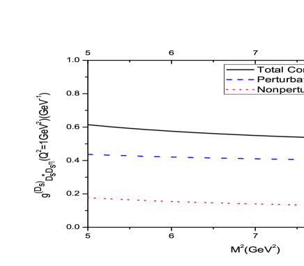
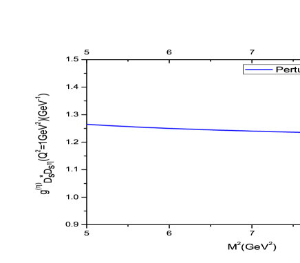
Figure 2: Left: $g^{(D_{s})}_{D_{s}^{*}D_{s}\eta}(Q^{2}=1~{}GeV^{2})$ as a function of the Borel mass parameter $M^{2}$. Right: $g^{(\eta)}_{D_{s}^{*}D_{s}\eta}(Q^{2}=1~{}GeV^{2})$ as a function of the Borel mass $M^{2}$.

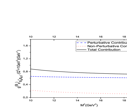
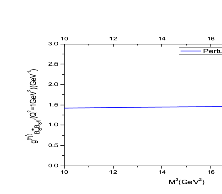
Figure 3: Left: $g^{(B_{s})}_{B_{s}^{*}B_{s}\eta^{\prime}}(Q^{2}=1~{}GeV^{2})$ as a function of the Borel mass $M^{2}$. Right: $g^{(\eta^{\prime})}_{B_{s}^{*}B_{s}\eta^{\prime}}(Q^{2}=1~{}GeV^{2})$ as a function of the Borel mass parameter $M^{2}$.

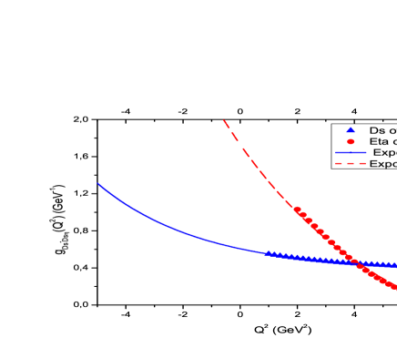
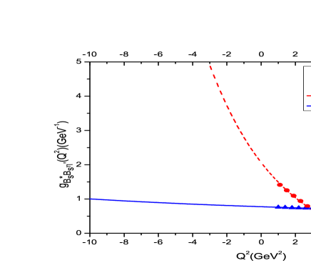
Figure 4: Left: $g_{D_{s}^{*}D_{s}\eta}(Q^{2})$ as a function of $Q^{2}$. Right: $g_{B_{s}^{*}B_{s}\eta^{\prime}}(Q^{2})$ as a function of $Q^{2}$.

$$\begin{array}[]{|c|c|c|c|}\hline\cr\hline\cr\mbox{ }&Q^{2}=-m_{D_{s}}^{2}&Q^{2}=-m_{\eta}^{2}&\mbox{Average}\par\\ \hline\cr\mbox{$g_{D_{s}^{*}D_{s}\eta}$}&1.06\pm 0.24&1.86\pm 0.36&1.46\pm 0.30\\ \hline\cr\hline\cr\mbox{ }&Q^{2}=-m_{D_{s}}^{2}&Q^{2}=-m_{\eta^{\prime}}^{2}&\mbox{Average}\par\\ \hline\cr\mbox{$g_{D_{s}^{*}D_{s}\eta^{\prime}}$}&0.62\pm 0.14&0.85\pm 0.18&0.74\pm 0.16\\ \hline\cr\hline\cr\hline\cr\mbox{ }&Q^{2}=-m_{B_{s}}^{2}&Q^{2}=-m_{\eta}^{2}&\mbox{Average}\par\\ \hline\cr\mbox{$g_{B_{s}^{*}B_{s}\eta}$}&4.54\pm 0.90&6.04\pm 1.22&5.29\pm 1.06\\ \hline\cr\hline\cr\mbox{ }&Q^{2}=-m_{B_{s}}^{2}&Q^{2}=-m_{\eta^{\prime}}^{2}&\mbox{Average}\par\\ \hline\cr\mbox{$g_{B_{s}^{*}B_{s}\eta^{\prime}}$}&2.06\pm 0.42&2.73\pm 0.54&2.29\pm 0.48\\ \hline\cr\hline\cr\end{array}$$

Table 3: The values of the coupling constants in $GeV^{-1}$ unit.

References

(1) P. del Amo Sanchez et al., (BABAR Collaboration), Phys. Rev. Lett. 105, 121801 (2010).
(2) H. Mendez et al., (CLEO Collaboration), Phys. Rev. D 81, 052013 (2010).
(3) D. Acosta et al., (CDF Collaboration), Phys. Rev. D71, 032001 (2005); Phys. Rev. Lett.94, 101803 (2005); T. Aaltonen, et al., (CDF Collaboration), Phys. Rev. Lett. 100, 082001 (2008).
(4) A. Abulenciaet et al., (CDF Collaboration), Phys. Rev. Lett. 97, 062003 (2006); Phys. Rev. Lett. 97, 242003 (2006).
(5) V.M. Abazov et al., (D0 Collaboration), Phys. Rev. Lett. 94, 042001 (2005); Phys. Rev. Lett. 98, 121801 (2007).
(6) T. Aaltonen, et al., (CDF Collaboration), Phys.Rev. D79, 092003(2009); T. Aaltonen, et al., (CDF Collaboration),
Phys.Rev. D77, 072003 (2008).
(7) M. A. Shifman, A. I. Vainshtein and V. I. Zakharov, Nucl. Phys. B 147, 385 (1979).
(8) M. E. Bracco, A. Cerqueira Jr., M. Chiapparini, A. Lozea, M. Nielsen, Phys. Lett. B 641, 286 (2006).
(9) Z. G. Wang, S. L. Wan, Phys. Rev. D 74, 014017 (2006).
(10) B. O. Rodrigues, M. E. Bracco, M. Nielsen, F. S. Navarra, arXiv:1003.2604v1[hep-ph].
(11) F.S. Navarra, M. Nielsen, M.E. Bracco, M. Chiapparini and C.L. Schat, Phys. Lett. B 489, 319 (2000).
(12) F. S. Navarra, M. Nielsen, M. E. Bracco, Phys. Rev. D 65, 037502 (2002).
(13) M. E. Bracco, M. Chiapparini, A. Lozea, F. S. Navarra and M. Nielsen, Phys. Lett. B 521, 1 (2001).
(14) R.D. Matheus, F.S. Navarra, M. Nielsen and R.R. da Silva, Phys. Lett. B 541, 265 (2002).
(15) R. D. Matheus, F. S. Navarra, M. Nielsen and R. Rodrigues da Silva, Int. J. Mod. Phys. E 14, 555 (2005).
(16) Z. G. Wang, Nucl. Phys. A 796, 61 (2007); Eur. Phys. J. C 52, 553 (2007);
(17) M. E. Bracco, M. Chiapparini, F. S. Navarra and M. Nielsen, Phys. Lett. B 605, 326 (2005).
(18) Z. G. Wang, Phys. Rev. D 77, 054024 (2008).
(19) P. Maris, P. C. Tandy, Phys. Rev. C 60, 055214 (1999).
(20) E. Gamiz, et al. (HPQCD Collab.), Phys. Rev. D 80, 014503 (2009).
(21) J. L. Rosner and S. Stone, arXiv:1002.1655 [hep-ex]; C. W. Hwang, Phys. Rev. D 81, 114024 (2010).
(22) W. Lucha, D. Melikhov and S. Simula, Phys. Rev. D 79, 0960011 (2009).
(23) F. S. Navarra, M. Nielsen, M. E. Bracco, Phys. Rev. D 65, 037502 (2002).
(24) M. E. Bracco, M. Chiapparini, F. S. Navarra, M. Nielsen, Phys. Lett. B 659, 559 (2008).
(25) L. B. Holanda, R. S. Marques de Carvalho and A. Mihara, Phys. Lett. B 644, 232 (2007).
(26) K. Azizi and H. Sundu, J. Phys. G: Nucl. Part. Phys. 38, 045005 (2011).
(27) C. Y. Cui, Y. L. Liu and M. Q. Huang, Phys. Lett. B 707, 129 (2012).
(28) S. V. Donskov, V. N. Kolosov, A. A. Lednev,
Yu. V. Mikhailov, V. A. Polyakov, V. D. Samoylenko, G. V.
Khaustov, IHEP 2012-22, arXiv:1301.6987
(29)J. Beringer et al., (Particle Data Group) Phys. Rev. D 86, 010001, (2012).
(30) D. Becirevic, et al., Phys. Rev. D 60, 074501 (1999).
(31) M. A. Ivanov and P. Santorelli, DSF-99-35, arXiv:9910434[hep-ph].
(32) G. Abbiendi et al. [OPAL Collaboration], Phys. Lett. B 516, 236-248 (2001).
(33) T. N. Pham, Phys. Lett. B 694, 129, (2010).
(34) B. L. Ioffe, Prog. Part. Nucl. Phys. 56, 232
(2006).