Stability Analysis of Continuous-Time Switched Systems with a Random Switching Signal

Abstract

This paper is concerned with the stability analysis of continuous-time switched systems with a random switching signal. The switching signal manifests its characteristics with that the dwell time in each subsystem consists of a fixed part and a random part. The stochastic stability of such switched systems is studied using a Lyapunov approach. A necessary and sufficient condition is established in terms of linear matrix inequalities. The effect of the random switching signal on system stability is illustrated by a numerical example and the results coincide with our intuition.

I Introduction

Generally speaking, a switched system is a dynamical system that consists of a finite number of subsystems and a switching signal. The subsystems are described by differential equations and are employed to capture the dominant dynamics of the system in different operation modes. The switching signal decides which subsystem is being activated (equivalently, which operation mode the system is working in) at a particular time. The study on switched systems has attracted a lot of research attention [1, 2, 3, 4]. Switched systems have various applications such as in communication networks [5], aerospace industry [6] and networked control systems [7, 8, 9]. The readers are referred to [10, 11] for a general introduction and [12] for a recent review.

A special class of switched systems with a random switching signal is Markovian jump systems where the switching signal is modeled by a Markov process [11]. The sliding mode control of Markovian jump systems has been studied in [13]. The filtering problem has been investigated in [14]. Some results of Markovian jump systems with time delays have been reported in [15]. When there are switching probability uncertainties, the stochastic stability problems have been studied in [16, 17, 18] recently.

In this paper, a new class of random switching signals is proposed to activate the subsystems of switched systems, and a necessary and sufficient condition is established for the stochastic stability analysis. For switched systems with the switching signal proposed in this paper, the dwell time in each subsystem consists of two parts: the fixed dwell time and the random dwell time. The fixed dwell time plays a similar role as the “dwell time” in deterministic switched systems [19]; the random dwell time is corresponding to the exponentially distributed “sojourn time” in Markovian jump systems [20]. With the proposed class of random switching signals, the switched system can be transformed to a Markovian jump system with state jumps at the switching time instants. The stochastic stability problem is then studied using a Lyapunov approach; and a necessary and sufficient condition is obtained. When the parameters of the random switching signal are known, the system stability can be checked by solving a set of coupled linear matrix inequalities. A numerical example is used to illustrate the effect of the random switching signals on system stability. The stability regions and instability regions are numerically determined for different values of the fixed dwell time parameters. The numerical results demonstrate that (1) when all the subsystems are stable, fast switching may destabilize the system, and hence it should be avoided; (2) when both stable and unstable subsystems are present, dwelling in the stable subsystems longer can increase the degree of the stability, otherwise the system will tend to become unstable; (3) when all the subsystems are unstable, both fast and slow switching can destabilize the system, the system stability, however, may sometimes be achieved by choosing the fixed dwell time parameters properly.

Compared to the previous work in [20, 15, 16, 6, 11, 14, 17, 18, 13], the work in this paper provides a new and more general view of switching, and the corresponding stability results. The class of random switching signals in this paper allows that a fixed dwell time can exist for each mode before a Markov switch occurs. Hence, the systems in this paper can possibly accommodate more realistic situations; the results in this paper should be applicable, in principle, to all previous cases. Moreover, the results in this paper also lay a foundation for novel hybrid controller design, which is illustrated by the numerical example in Section IV.

Notation: $\mathbb{R}^{n}$ and $\mathbb{S}^{+}$ are, respectively, the $n$-dimensional Euclidean space and the set of $n\times n$ real symmetric positive definite matrices. Notation $X<Y$, where $X$ and $Y$ are real symmetric matrices, means that the matrix $X-Y$ is negative definite. The superscript “$T$” denotes the transpose for vectors or matrices. $\left\lVert\cdot\right\rVert$ refers to the Euclidean norm for vectors. $\overline{\sigma}(\cdot)$ and $\underline{\sigma}(\cdot)$ are, respectively, the maximum and the minimum singular values of square matrices. Moreover, let $(\Omega,\mathcal{F},\mathrm{Pr})$ be a complete probability space. $\operatorname{E}\{\cdot\}$ and $\sigma\{\cdot\}$ stand for the expectation and the generated $\sigma$-algebra, respectively.

II Problem Formulation

Consider a class of switched linear systems defined on a complete probability space $(\Omega,\mathcal{F},\mathrm{Pr})$

$$\dot{x}(t)=A_{r(t)}x(t)$$ (1)

where $x(t)\in\mathbb{R}^{n}$, $t\geq 0$, is the system state, $r(t)\in\mathcal{M}\triangleq\left\{1,2,\ldots,m\right\}$ is the switching signal deciding the current system operation mode. Suppose the system switches its operation mode to $i\in\mathcal{M}$ at time $t_{k}$, the characteristic of the switching signal $r(t)$ can be described as follows. For time $t\in[t_{k},t_{k}+d_{i})$, where $d_{i}\geq 0$, no switching is allowed almost surely; that is,

$$\Pr\left\{r(t+\Delta t)=j\mid r(t)=i\right\}=\left\{\begin{aligned} &0,\text{ if $j\neq i$}\\ &1,\text{ if $j=i$}\end{aligned}\right.$$ (2)

where $\Delta t$ is a small time increment satisfying $\lim_{\Delta t\to 0^{+}}\frac{o(\Delta t)}{\Delta t}=0$. The parameter $d_{i}$ plays the role of “dwell time” in deterministic switched systems[19], and is called the fixed dwell time of the system in (1). For $t\geq t_{k}+d_{i}$, mode switching occurs according to the mode transition probabilities given by

$$\Pr\left\{r(t+\Delta t)=j\mid r(t)=i\right\}=\left\{\begin{aligned} &\pi_{ij}\Delta t+o(\Delta t),\text{if $j\neq i$}\\ &1+\pi_{ii}\Delta t+o(\Delta t),\text{if $j=i$}\end{aligned}\right.$$ (3)

where $\pi_{ij}\geq 0$ if $j\neq i$, and $\pi_{ii}\triangleq-\sum_{j=1,j\neq i}^{m}\pi_{ij}$ if $j=i$. If the next switching occurs at time $t_{k+1}$, we can define $\eta_{i}\triangleq t_{k+1}-(t_{k}+d_{i})$, which is an exponential random variable with parameter $v_{i}\triangleq-\pi_{ii}$ according to (3). To simplify the derivation of the main results, the system (1) is assumed to have no absorbing mode; that is, $\pi_{ii}\neq 0$ for all $i\in\mathcal{M}$. The random variable $\eta_{i}$ plays the role of “sojourn time” in Markovian jump systems[11, 20], and is called the random dwell time of the system. The dwell time of system (1) in mode $i$ is defined as $\tau_{i}\triangleq t_{k+1}-t_{k}=d_{i}+\eta_{i}$, indicating the total time length of the system (1) being in mode $i$. As a result, the time interval $[t_{k},t_{k+1})$ can be correspondingly divided into two parts: $[t_{k},t_{k+1})=[t_{k},t_{k}+d_{i})\cup[t_{k}+d_{i},t_{k+1})$. It can be seen from above that $t_{0}=0$, $t_{k+1}>t_{k}$ and $\lim_{k\to\infty}t_{k}=\infty$.

Example 1

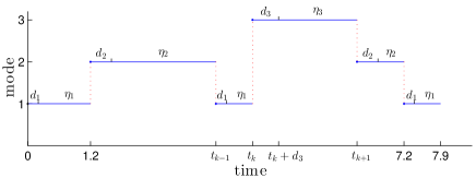
Let us illustrate the property of the switching signal $r(t)$ with an example. Suppose $r(t)\in\left\{1,2,3\right\}$. A sample path of $r(t)$ is illustrated in Fig. 1. Here, the system changes its mode at time $t_{k}$ from Mode 1 to Mode 3. In view of (2), there will be no switching almost surely during the interval $[t_{k},t_{k}+d_{3})$; the system is allowed to switch modes after the time $t_{k}+d_{3}$ and obeys the switching rule in (3).

Figure 1: A sample path of the random switching signal

Definition 1

Let $x(t)$ be the state trajectory of system (1). Then system (1) is said to be stochastically stable if

$$\operatorname{E}\left\{\int_{0}^{\infty}\left\lVert x(t)\right\rVert^{2}dt\mid x_{0},r_{0}\right\}<\infty$$ (4)

for any initial system state $x_{0}\in\mathbb{R}^{n}$ and any initial operation mode $r_{0}\in\mathcal{M}$.

Remark 1

The above stochastic stability definition is analogous to that of Markovian jump systems [20]. It is also a uniform stability in the sense that the inequality (4) is required to be true over all the switching signals defined by (2)–(3).

III Stability Analysis

The stability property of the system in (1) is studied via two steps. In Step 1, the stochastic stability of the system in (1) is shown to be equivalent to the stochastic stability of an auxiliary system. In Step 2, the stability of the auxiliary system is studied by a Lyapunov approach, and a necessary and sufficient condition is established.

III-A Switched Systems with State Jumps

A switched system with state jumps is the auxiliary system to be constructed in this section. The stability of the constructed auxiliary system is shown to be equivalent to that of the system in (1).

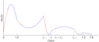
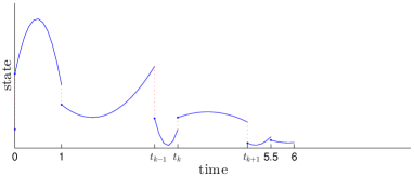
Let us first study the state trajectory of system (1) to motivate the construction of the auxiliary system. A sample path of the state trajectory of system (1) is illustrated in Fig. 2. Suppose the system switches to mode $r_{k}\in\mathcal{M}$ at time $t_{k}$. Then the system state $x(t)$ will evolve from $x(t_{k})$ at time $t_{k}$ to $x(t_{k}+d_{r_{k}})=e^{A_{r_{k}}d_{r_{k}}}x(t_{k})$ at time $t_{k}+d_{r_{k}}$ almost surely. The idea here is to squeeze the interval $[t_{k},t_{k}+d_{r_{k}})$ to a point $t_{k}$ and make the system in (1) having a state jump from $x(t_{k}^{-})$ to $e^{A_{r_{k}}d_{r_{k}}}x(t_{k}^{-})$ at time $t_{k}$, as illustrated in Fig. 3, where $x(t_{k}^{-})\triangleq\lim_{t\to t_{k}^{-}}x(t)$.

Figure 2: State trajectory of the switched systems

Figure 3: State trajectory of the switched systems with state jumps

As a result, the system in (1) can be transformed to a randomly switched system with state jumps:

$$\left\{\begin{aligned} \dot{\xi}(\tilde{t})&=A_{\rho(\tilde{t})}\xi(\tilde{t}),\qquad\quad\tilde{t}_{k}<\tilde{t}<\tilde{t}_{k+1}\\ \xi(\tilde{t}_{k})&=e^{A_{\rho_{k}}d_{\rho_{k}}}\xi(\tilde{t}_{k}^{-}),\quad k=0,1,2,\ldots\end{aligned}\right.$$ (5)

where $\xi(\tilde{t})$ is the system state, $\tilde{t}_{k}$, $k=0,1,2,\ldots$, are the time instants when the system switches its operation modes. $\xi(\tilde{t}_{k}^{-})\triangleq\lim_{t\to t_{k}^{-}}\xi(\tilde{t})$ is the system state just before switches. $\rho(\tilde{t})$ is a Markovian process taking values in $\mathcal{M}$ and equipped with the transition probabilities

$$\Pr\left\{\rho(\tilde{t}+\Delta t)=j\mid\rho(\tilde{t})=i\right\}=\left\{\begin{aligned} &\pi_{ij}\Delta t+o(\Delta t),\text{if $j\neq i$}\\ &1+\pi_{ii}\Delta t+o(\Delta t),\text{if $j=i$}\end{aligned}\right.$$ (6)

where $\pi_{ij}$ are the same as those in (3). The mode transition rate matrix is denoted by $\Pi\triangleq(\pi_{ij})\in\mathbb{R}^{m\times m}$. Suppose that the system (5) jumps to mode $\rho_{k}\triangleq\rho(\tilde{t}_{k})$ at time $\tilde{t}_{k}$, the dwell time of system (5) in mode $\rho_{k}$ is defined as $\eta_{\rho_{k}}\triangleq\tilde{t}_{k+1}-\tilde{t}_{k}$. It follows from (6) that $\eta_{\rho_{k}}$ is an exponentially distributed random variable with parameter $v_{\rho_{k}}$. In other words, $\eta_{\rho_{k}}$ has the same distribution as the corresponding random dwell time in (3). Also, we have that $\tilde{t}_{0}=0$, $\tilde{t}_{k+1}>\tilde{t}_{k}$, $\lim_{k\to\infty}\tilde{t}_{k}=\infty$ and $\tilde{t}_{k+1}=\sum_{l=0}^{k}\eta_{\rho_{l}}$.

For the systems in (1) and (5), we define the filtrations $\mathcal{F}_{t}\triangleq\sigma\left\{(x(\tau),r(\tau)):0\leq\tau\leq t\right\}$ and $\mathcal{G}_{t}\triangleq\sigma\left\{(\xi(\tau),\rho(\tau)):0\leq\tau\leq t\right\}$ for $t\geq 0$, respectively. Now we are ready to establish the equivalence of the stability properties between system (1) and system (5).

Lemma 1

The stochastic stability of the system in (1) is equivalent to the stochastic stability of the system in (5).

Proof:

The equivalence is proved based on the following observation: Given any sample path $(\xi(\tilde{t}),\rho(\tilde{t}))$ of the system in (5), there is a corresponding sample path $(x(t),r(t))$ of the system in (1); and vice versa. Furthermore, the two sample paths satisfy the following properties: For $k=0,1,2,\ldots$,

1. $x(0)=\xi(0^{-})$, $\xi(0)=e^{A_{\rho_{0}}d_{\rho_{0}}}\xi(0^{-})$ and $t_{0}=\tilde{t}_{0}=0$.

2. $r_{k}=r(t_{k})=\rho(\tilde{t}_{k})=\rho_{k}$.

3. $t_{k+1}=\sum_{l=0}^{k}(d_{\rho_{l}}+\eta_{\rho_{l}})=\tilde{t}_{k+1}+\sum_{l=0}^{k}d_{\rho_{l}}$.

4. $\xi(\tilde{t}_{k}+\tau)=x(t_{k}+d_{r_{k}}+\tau)$ for $0\leq\tau<\eta_{\rho_{k}}$.

The fourth property is a direct result of the first three properties; that is, $\xi(\tilde{t}_{k}+\tau)=e^{A_{\rho_{k}}\tau}\xi(\tilde{t}_{k})=e^{A_{\rho_{k}}\tau}e^{A_{\rho_{k}}d_{\rho_{k}}}\xi(\tilde{t}_{k}^{-})=e^{A_{r_{k}}(d_{r_{k}}+\tau)}x(t_{k})=x(t_{k}+d_{r_{k}}+\tau)$.

($\Rightarrow$) Suppose that the system in (1) is stochastically stable, the stability of the system in (5) follows from

$$\quad\operatorname{E}\left\{\int_{0}^{\infty}\left\lVert\xi(\tilde{t})\right\rVert^{2}d\tilde{t}\mid\xi_{0},\rho_{0}\right\}$$

$$=\operatorname{E}\left\{\sum_{k=0}^{\infty}\left\{\int_{\tilde{t}_{k}}^{\tilde{t}_{k+1}}\left\lVert\xi(\tilde{t})\right\rVert^{2}d\tilde{t}\right\}\mid\xi_{0},\rho_{0}\right\}$$

$$=\operatorname{E}\left\{\sum_{k=0}^{\infty}\left\{\int_{t_{k}+d_{r_{k}}}^{t_{k+1}}\left\lVert x(t)\right\rVert^{2}dt\right\}\mid x_{0},r_{0}\right\}$$

$$\leq\operatorname{E}\left\{\sum_{k=0}^{\infty}\left\{\int_{t_{k}}^{t_{k+1}}\left\lVert x(t)\right\rVert^{2}dt\right\}\mid x_{0},r_{0}\right\}$$

$$=\operatorname{E}\left\{\int_{0}^{\infty}\left\lVert x(t)\right\rVert^{2}dt\mid x_{0},r_{0}\right\}<\infty$$

The second “$=$” holds because of the fourth property of the two sample paths.

($\Leftarrow$) Suppose that the system in (5) is stochastically stable. Note that $\eta_{r_{k}}$ is an exponential random variable with parameter $v_{r_{k}}$. In view of Lemma 2 and Lemma 3 (see Appendix), there exists a real number $c_{r_{k}}<v_{r_{k}}$ such that

$$\quad\operatorname{E}\left\{\int_{t_{k}+d_{r_{k}}}^{t_{k+1}}\left\lVert x(t)\right\rVert^{2}dt\mid\mathcal{F}_{t_{k}}\right\}$$

$$=\operatorname{E}\left\{\int_{t_{k}+d_{r_{k}}}^{t_{k+1}}\left\lVert x(t)\right\rVert^{2}dt\mid x(t_{k}),r(t_{k})=r_{k}\right\}$$

$$=\operatorname{E}\left\{\int_{t_{k}+d_{r_{k}}}^{t_{k}+d_{r_{k}}+\eta_{r_{k}}}\left\lVert e^{A_{r_{k}}(t-t_{k})}x(t_{k})\right\rVert^{2}dt\right\}$$

$$=\operatorname{E}\left\{\int_{d_{r_{k}}}^{d_{r_{k}}+\eta_{r_{k}}}\left\lVert e^{A_{r_{k}}\tau}x(t_{k})\right\rVert^{2}d\tau\right\}$$

$$\geq\operatorname{E}\left\{\int_{d_{r_{k}}}^{d_{r_{k}}+\eta_{r_{k}}}e^{c_{r_{k}}\tau}\left\lVert x(t_{k})\right\rVert^{2}d\tau\right\}$$

$$=\operatorname{E}\left\{\int_{d_{r_{k}}}^{d_{r_{k}}+\eta_{r_{k}}}e^{c_{r_{k}}\tau}d\tau\right\}\left\lVert x(t_{k})\right\rVert^{2}$$

$$=\frac{e^{v_{r_{k}}d_{r_{k}}}}{v_{r_{k}}-c_{r_{k}}}\left\lVert x(t_{k})\right\rVert^{2}\geq\alpha_{\mathrm{min}}\left\lVert x(t_{k})\right\rVert^{2}$$ (7)

for any $x(t_{k})\neq 0$ and any $r_{k}\in\mathcal{M}$, where $\alpha_{\mathrm{min}}\triangleq\min_{i\in\mathcal{M}}\left\{\frac{e^{v_{i}d_{i}}}{v_{i}-c_{i}}\right\}>0$. The first “$=$” holds due to the property of the process $(x(t),r(t))$, the first “$\geq$” holds because of Lemma 2, and the last “$=$” holds because of Lemma 3. Now, we have

$$\quad\operatorname{E}\left\{\int_{t_{k}}^{t_{k}+d_{r_{k}}}\left\lVert x(t)\right\rVert^{2}dt\mid\mathcal{F}_{t_{k}}\right\}$$

$$=\operatorname{E}\left\{\int_{t_{k}}^{t_{k}+d_{r_{k}}}\left\lVert x(t)\right\rVert^{2}dt\mid x(t_{k}),r(t_{k})=r_{k}\right\}$$

$$=\int_{t_{k}}^{t_{k}+d_{r_{k}}}\left\lVert e^{A_{r_{k}}(t-t_{k})}x(t_{k})\right\rVert^{2}dt$$

$$=\int_{0}^{d_{r_{k}}}\left\lVert e^{A_{r_{k}}\tau}x(t_{k})\right\rVert^{2}d\tau$$

$$\leq\int_{0}^{d_{r_{k}}}\alpha_{\mathrm{max}}\left\lVert x(t_{k})\right\rVert^{2}d\tau$$

$$\leq d_{\mathrm{max}}\alpha_{\mathrm{max}}\left\lVert x(t_{k})\right\rVert^{2}$$

$$\leq\frac{d_{\mathrm{max}}\alpha_{\mathrm{max}}}{\alpha_{\mathrm{min}}}\operatorname{E}\left\{\int_{t_{k}+d_{r_{k}}}^{t_{k+1}}\left\lVert x(t)\right\rVert^{2}dt\mid\mathcal{F}_{t_{k}}\right\}$$ (8)

where $\alpha_{\mathrm{max}}\triangleq\max_{i\in\mathcal{M}}\left\{\max_{\tau\in[0,d_{i}]}\overline{\sigma}^{2}\left(e^{A_{i}\tau}\right)\right\}$ and $d_{\mathrm{max}}\triangleq\max_{i\in\mathcal{M}}\{d_{i}\}$. The last “$\leq$” holds because of (7). Therefore,

$$\quad\operatorname{E}\left\{\int_{t_{k}}^{t_{k+1}}\left\lVert x(t)\right\rVert^{2}dt\mid\mathcal{F}_{t_{k}}\right\}$$

$$=\operatorname{E}\left\{\int_{t_{k}}^{t_{k}+d_{r_{k}}}\left\lVert x(t)\right\rVert^{2}dt\mid\mathcal{F}_{t_{k}}\right\}+\operatorname{E}\left\{\int_{t_{k}+d_{r_{k}}}^{t_{k+1}}\left\lVert x(t)\right\rVert^{2}dt\mid\mathcal{F}_{t_{k}}\right\}$$

$$\leq\left[\frac{d_{\mathrm{max}}\alpha_{\mathrm{max}}}{\alpha_{\mathrm{min}}}+1\right]\operatorname{E}\left\{\int_{t_{k}+d_{r_{k}}}^{t_{k+1}}\left\lVert x(t)\right\rVert^{2}dt\mid\mathcal{F}_{t_{k}}\right\}$$

$$=\left[\frac{d_{\mathrm{max}}\alpha_{\mathrm{max}}}{\alpha_{\mathrm{min}}}+1\right]\operatorname{E}\left\{\int_{\tilde{t}_{k}}^{\tilde{t}_{k+1}}\left\lVert\xi(\tilde{t})\right\rVert^{2}d\tilde{t}\mid\mathcal{G}_{\tilde{t}_{k}}\right\}$$ (9)

Here, the “$\leq$” holds because of (8), and the last “$=$” holds because of the four properties stated in the beginning of the proof.

But, by the property of the conditional expectation, we have

$$\operatorname{E}\left\{\operatorname{E}\left\{\int_{t_{k}}^{t_{k+1}}\left\lVert x(t)\right\rVert^{2}dt\mid\mathcal{F}_{t_{k}}\right\}\mid x_{0},r_{0}\right\}$$

$$\qquad\qquad=\operatorname{E}\left\{\int_{t_{k}}^{t_{k+1}}\left\lVert x(t)\right\rVert^{2}dt\mid x_{0},r_{0}\right\}$$

and

$$\operatorname{E}\left\{\operatorname{E}\left\{\int_{\tilde{t}_{k}}^{\tilde{t}_{k+1}}\left\lVert\xi(\tilde{t})\right\rVert^{2}d\tilde{t}\mid\mathcal{G}_{\tilde{t}_{k}}\right\}\mid\xi_{0},\rho_{0}\right\}$$

$$\qquad\qquad=\operatorname{E}\left\{\int_{\tilde{t}_{k}}^{\tilde{t}_{k+1}}\left\lVert\xi(\tilde{t})\right\rVert^{2}d\tilde{t}\mid\xi_{0},\rho_{0}\right\}$$

Taking the conditional expectation on both sides of (9), we have

$$\operatorname{E}\left\{\int_{t_{k}}^{t_{k+1}}\left\lVert x(t)\right\rVert^{2}dt\mid x_{0},r_{0}\right\}$$

$$\qquad\qquad\leq\left[\frac{d_{\mathrm{max}}\alpha_{\mathrm{max}}}{\alpha_{\mathrm{min}}}+1\right]\operatorname{E}\left\{\int_{\tilde{t}_{k}}^{\tilde{t}_{k+1}}\left\lVert\xi(\tilde{t})\right\rVert^{2}d\tilde{t}\mid\xi_{0},\rho_{0}\right\}$$

Finally, the stability of the system in (5) implies that

$$\quad\operatorname{E}\left\{\int_{0}^{\infty}\left\lVert x(t)\right\rVert^{2}dt\mid x_{0},r_{0}\right\}$$

$$=\operatorname{E}\left\{\sum_{k=0}^{\infty}\int_{t_{k}}^{t_{k+1}}\left\lVert x(t)\right\rVert^{2}dt\mid x_{0},r_{0}\right\}$$

$$=\sum_{k=0}^{\infty}\operatorname{E}\left\{\int_{t_{k}}^{t_{k+1}}\left\lVert x(t)\right\rVert^{2}dt\mid x_{0},r_{0}\right\}$$

$$\leq\left[\frac{d_{\mathrm{max}}\alpha_{\mathrm{max}}}{\alpha_{\mathrm{min}}}+1\right]\sum_{k=0}^{\infty}\operatorname{E}\left\{\int_{\tilde{t}_{k}}^{\tilde{t}_{k+1}}\left\lVert\xi(\tilde{t})\right\rVert^{2}d\tilde{t}\mid\xi_{0},\rho_{0}\right\}$$

$$=\left[\frac{d_{\mathrm{max}}\alpha_{\mathrm{max}}}{\alpha_{\mathrm{min}}}+1\right]\operatorname{E}\left\{\int_{0}^{\infty}\left\lVert\xi(\tilde{t})\right\rVert^{2}d\tilde{t}\mid\xi_{0},\rho_{0}\right\}$$

$$<\infty$$

Therefore, the system in (1) is stochastically stable. ∎

Remark 2

Lemma 1 still holds if the assumption of no absorbing mode existing in the system is removed. In this case, the proof is still valid before the systems enter a absorbing mode. Once the systems enter a absorbing mode, the subsystem corresponding to the absorbing mode must be a stable subsystem.

In view of Lemma 1, the study of stability of the system in (1) is transferred to the stability study of system (5). Since the switching signal of system (5) is a Markov process, the stability analysis becomes solvable.

III-B Stability Result

In this section, a necessary and sufficient condition is derived for the stochastic stability analysis of system (1) based upon Lemma 1.

Theorem 1

System (1) is stochastically stable if and only if there exist matrices $P_{i}\in\mathbb{S}^{+}$, $i\in\mathcal{M}$, such that

$$A_{i}^{T}P_{i}+P_{i}A_{i}+\pi_{ii}P_{i}+\sum_{j=1,j\neq i}^{m}\left\{\pi_{ij}e^{A_{j}^{T}d_{j}}P_{j}e^{A_{j}d_{j}}\right\}<0$$ (10)

for all $i\in\mathcal{M}$.

Proof:

($\Leftarrow$) Suppose that there exist matrices $P_{i}\in\mathbb{S}^{+}$ such that (10) holds for all $i\in\mathcal{M}$, we shall show that the system in (5) is stochastically stable. Consider the Lyapunov function

$$V(\xi(\tilde{t}),\rho(\tilde{t}))\triangleq\xi^{T}(\tilde{t})P(\rho(\tilde{t}))\xi(\tilde{t})$$

where $P(\rho(\tilde{t})=i)\triangleq P_{i}>0$. It follows from (5) and (6) that

$$\Pr\left\{\xi(\tilde{t}+\Delta t)=e^{A_{j}d_{j}}[\xi(\tilde{t})+A_{j}\xi(\tilde{t})\Delta t]+o(\Delta t)\mid\xi(\tilde{t}),\rho(\tilde{t})=i\right\}$$

$$\qquad\qquad\qquad\qquad\qquad=\pi_{ij}\Delta t+o(\Delta t),\text{ if $j\neq i$}$$ (11)

$$\Pr\left\{\xi(\tilde{t}+\Delta t)=\xi(\tilde{t})+A_{i}\xi(\tilde{t})\Delta t+o(\Delta t)\mid\xi(\tilde{t}),\rho(\tilde{t})=i\right\}$$

$$\qquad\qquad\qquad\qquad\qquad=1+\pi_{ii}\Delta t+o(\Delta t),\text{ if $j=i$}$$ (12)

$$\Pr\left\{P(\rho(\tilde{t}+\Delta t))=P_{j}\mid\xi(\tilde{t}),\rho(\tilde{t})=i\right\}$$

$$\qquad\qquad\qquad\qquad\qquad=\pi_{ij}\Delta t+o(\Delta t),\text{ if $j\neq i$}$$ (13)

$$\Pr\left\{P(\rho(\tilde{t}+\Delta t))=P_{i}\mid\xi(\tilde{t}),\rho(\tilde{t})=i\right\}$$

$$\qquad\qquad\qquad\qquad\qquad=1+\pi_{ii}\Delta t+o(\Delta t),\text{ if $j=i$}$$ (14)

In (11), $\xi(\tilde{t})$ is considered as the system state just before the mode switches. At the switching time, the system state jumps from $\xi(\tilde{t})$ to $e^{A_{j}d_{j}}\xi(\tilde{t})$. After the switching, the system state change is given by $A_{j}e^{A_{j}d_{j}}\xi(\tilde{t})\Delta t+o(\Delta t)$.

Let $R_{i}\triangleq A_{i}^{T}P_{i}+P_{i}A_{i}+\pi_{ii}P_{i}+\sum_{j=1,j\neq i}^{m}\pi_{ij}e^{A_{j}^{T}d_{j}}P_{j}e^{A_{j}d_{j}}$. It follows from (11)–(14) that

$$\quad\operatorname{E}\left\{V(\xi(\tilde{t}+\Delta t),\rho(\tilde{t}+\Delta t))\mid\xi(\tilde{t}),\rho(\tilde{t})=i\right\}$$

$$=\operatorname{E}\left\{\xi^{T}(\tilde{t}+\Delta t)P(\rho(\tilde{t}+\Delta t))\xi(\tilde{t}+\Delta t)\mid\xi(\tilde{t}),\rho(\tilde{t})=i\right\}$$

$$=[1+\pi_{ii}\Delta t][\xi(\tilde{t})+A_{i}\xi(\tilde{t})\Delta t]^{T}P_{i}[\xi(\tilde{t})+A_{i}\xi(\tilde{t})\Delta t]$$

$$\quad+\sum_{j=1,j\neq i}^{m}\left\{[\pi_{ij}\Delta t][\xi(\tilde{t})+A_{j}\xi(\tilde{t})\Delta t]^{T}e^{A_{j}^{T}d_{j}}P_{j}e^{A_{j}d_{j}}\right.$$

$$\qquad\qquad\qquad\left.\times[\xi(\tilde{t})+A_{j}\xi(\tilde{t})\Delta t]\right\}+o(\Delta t)$$

$$=\xi^{T}(\tilde{t})[P_{i}+R_{i}\Delta t]\xi(\tilde{t})+o(\Delta t)$$

Therefore, the infinitesimal generator of $V(\xi(\tilde{t}),\rho(\tilde{t}))$ is given by

$$\quad\mathcal{L}V(\xi(\tilde{t}),\rho(\tilde{t})=i)$$

$$\triangleq\lim_{\Delta t\to 0^{+}}\frac{1}{\Delta t}\left[\operatorname{E}\left\{V(\xi(\tilde{t}+\Delta t),\rho(\tilde{t}+\Delta t))\mid\xi(\tilde{t}),\rho(\tilde{t})=i\right\}\right.$$

$$\qquad\qquad\qquad\left.-V(\xi(\tilde{t}),\rho(\tilde{t})=i)\right]$$

$$=\xi^{T}(\tilde{t})R_{i}\xi(\tilde{t})=-\xi^{T}(\tilde{t})(-R_{i})\xi(\tilde{t})\leq-\beta\left\lVert\xi(\tilde{t})\right\rVert^{2}$$ (15)

for any $\rho(\tilde{t})=i\in\mathcal{M}$, where $\beta\triangleq\min_{i\in\mathcal{M}}\left\{\underline{\sigma}(-R_{i})\right\}>0$.

From (15), we obtain

$$\lim_{\tilde{t}\to\infty}\operatorname{E}\left\{V(\xi(\tilde{t}),\rho(\tilde{t}))\mid\xi_{0},\rho_{0}\right\}=0$$

and

$$\left\lVert\xi(\tilde{t})\right\rVert^{2} \leq-\frac{1}{\beta}\mathcal{L}V(\xi(\tilde{t}),\rho(\tilde{t}))$$

for any $\xi(\tilde{t})\neq 0$ and any $\rho(\tilde{t})\in\mathcal{M}$. By Dynkin’s formula [21], we have

$$\quad\operatorname{E}\left\{\int_{0}^{\infty}\left\lVert\xi(\tilde{t})\right\rVert^{2}dt\mid\xi_{0},\rho_{0}\right\}$$

$$\leq-\frac{1}{\beta}\operatorname{E}\left\{\int_{0}^{\infty}\mathcal{L}V(\xi(\tilde{t}),\rho(\tilde{t}))dt\mid\xi_{0},\rho_{0}\right\}$$

$$=-\frac{1}{\beta}\left[\operatorname{E}\left\{\lim_{\tilde{t}\to\infty}V(\xi(\tilde{t}),\rho(\tilde{t}))\mid\xi_{0},\rho_{0}\right\}-V(\xi_{0},\rho_{0})\right]$$

$$\leq\frac{1}{\beta}V(\xi_{0},\rho_{0})<\infty$$

for any $\xi_{0}\neq 0$ and $\rho_{0}\in\mathcal{M}$. Therefore, the system in (5) is stochastically stable, and so is the system in (1) in view of Lemma 1.

($\Rightarrow$) According to Lemma 1, the stochastic stability of the system in (1) implies the stochastic stability of the system in (5). We will show that there exist matrices $P_{i}\in\mathbb{S}^{+}$ such that (10) holds for all $i\in\mathcal{M}$. Let $\xi(\tilde{t})$ be the state trajectory of the system in (5). Given any $\xi(\tilde{t})\neq 0$, $\rho(\tilde{t})\in\mathcal{M}$ and $Q_{i}\in\mathbb{S}^{+}$, $i\in\mathcal{M}$, define a matrix-valued function $P(\omega-\tilde{t},\rho(\tilde{t}))$ of $\omega$ and $\rho(\tilde{t})$ such that

$$\xi^{T}(\tilde{t})P(\omega-\tilde{t},\rho(\tilde{t}))\xi(\tilde{t})=\operatorname{E}\left\{\int_{\tilde{t}}^{\omega}\xi^{T}(\tau)Q(\rho(\tau))\xi(\tau)d\tau\mid\xi(\tilde{t}),\rho(\tilde{t})\right\}$$ (16)

where $Q(\rho(\tau)=i)\triangleq Q_{i}$. The quadratic form on the left side of (16) is non-decreasing as $\omega$ increases since $Q_{i}>0$. It is also bounded from above as $\omega\to\infty$ since the system in (5) is stochastically stable. Thus $\lim_{\omega\to\infty}\xi^{T}(\tilde{t})P(\omega-\tilde{t},\rho(\tilde{t}))\xi(\tilde{t})$ exists. We can define a new matrix-valued function $P(\rho(\tilde{t}))$ of $\rho(\tilde{t})$ such that

$$\xi^{T}(\tilde{t})P(\rho(\tilde{t}))\xi(\tilde{t}) =\lim_{\omega\to\infty}\xi^{T}(\tilde{t})P(\omega-\tilde{t},\rho(\tilde{t}))\xi(\tilde{t})>0$$

for any $\xi(\tilde{t})\neq 0$ and $\rho(\tilde{t})\in\mathcal{M}$. Therefore, we have

$$P(\rho(\tilde{t}))=\lim_{\omega\to\infty}P(\omega-\tilde{t},\rho(\tilde{t}))>0$$ (17)

We have constructed a set of matrices $P_{i}\triangleq P(\rho(\tilde{t})=i)\in\mathbb{S}^{+}$ for all $i\in\mathcal{M}$. In the following, we show that $P_{i}$ are solutions to (10).

It follows from (16) that

$$\operatorname{E}\left\{\xi^{T}(\tilde{t})P(\omega-\tilde{t},\rho(\tilde{t}))\xi(\tilde{t})-\xi^{T}(\tilde{t}+\Delta t)P(\omega-\tilde{t}-\Delta t,\rho(\tilde{t}+\Delta t))\right.$$

$$\qquad\quad\left.\times\xi(\tilde{t}+\Delta t)\mid\xi(\tilde{t}),\rho(\tilde{t})\right\}$$

$$=\operatorname{E}\left\{\operatorname{E}\left\{\int_{\tilde{t}}^{\omega}\xi^{T}(\tau)Q(\rho(\tau))\xi(\tau)d\tau\mid\xi(\tilde{t}),\rho(\tilde{t})\right\}\right.$$

$$\qquad\qquad\left.-\operatorname{E}\left\{\int_{\tilde{t}+\Delta t}^{\omega}\xi^{T}(\tau)Q(\rho(\tau))\xi(\tau)d\tau\mid\xi(\tilde{t}+\Delta t),\rho(\tilde{t}+\Delta t)\right\}\right.$$

$$\qquad\qquad\qquad\qquad\left.\mid\xi(\tilde{t}),\rho(\tilde{t})\right\}$$

$$=\operatorname{E}\left\{\int_{\tilde{t}}^{\omega}\xi^{T}(\tau)Q(\rho(\tau))\xi(\tau)d\tau\mid\xi(\tilde{t}),\rho(\tilde{t})\right\}$$

$$\qquad-\operatorname{E}\left\{\int_{\tilde{t}+\Delta t}^{\omega}\xi^{T}(\tau)Q(\rho(\tau))\xi(\tau)d\tau\mid\xi(\tilde{t}),\rho(\tilde{t})\right\}$$

$$=\operatorname{E}\left\{\int_{\tilde{t}}^{\tilde{t}+\Delta t}\xi^{T}(\tau)Q(\rho(\tau))\xi(\tau)d\tau\mid\xi(\tilde{t}),\rho(\tilde{t})\right\}$$

$$=\xi^{T}(\tilde{t})\left[P(\omega-\tilde{t},i)-P(\omega-\tilde{t}-\Delta t,i)-A_{i}^{T}P(\omega-\tilde{t}-\Delta t,i)\Delta t\right.$$

$$\qquad\quad-P(\omega-\tilde{t}-\Delta t,i)A_{i}\Delta t-[\pi_{ii}\Delta t]P(\omega-\tilde{t}-\Delta t,i)$$

$$\qquad\quad\left.-\sum_{j=1,j\neq i}^{m}\left\{[\pi_{ij}\Delta t]e^{A_{j}^{T}d_{j}}P(\omega-\tilde{t}-\Delta t,j)e^{A_{j}d_{j}}\right\}\right]\xi(\tilde{t})$$

$$\qquad+o(\Delta t)$$ (18)

The second “$=$” holds because $(\xi(\tilde{t}),\rho(\tilde{t}))$ is a Markov process; the last “$=$” follows from the direct calculation of

$$\operatorname{E}\left\{\xi^{T}(\tilde{t}+\Delta t)P(\omega-\tilde{t}-\Delta t,\rho(\tilde{t}+\Delta t))\xi(\tilde{t}+\Delta t)\mid\xi(\tilde{t}),\rho(\tilde{t})=i\right\}$$

$$=[1+\pi_{ii}\Delta t][\xi(\tilde{t})+A_{i}\xi(\tilde{t})\Delta t]^{T}P(\omega-\tilde{t}-\Delta t,i)[\xi(\tilde{t})+A_{i}\xi(\tilde{t})\Delta t]$$

$$\quad+\sum_{j=1,j\neq i}^{m}\left\{[\pi_{ij}\Delta t][\xi(\tilde{t})+A_{j}\xi(\tilde{t})\Delta t]^{T}e^{A_{j}^{T}d_{j}}P(\omega-\tilde{t}-\Delta t,j)\right.$$

$$\quad\qquad\qquad\quad\left.\times e^{A_{j}d_{j}}[\xi(\tilde{t})+A_{j}\xi(\tilde{t})\Delta t]\right\}+o(\Delta t)$$

It follows from (17) that $\lim_{\omega\to\infty}P(\omega-\tilde{t},i)=P_{i}$ and $\lim_{\omega\to\infty}P(\omega-\tilde{t}-\Delta t,j)=P_{j}$. Taking limit on the right side of (18) as $\omega\to\infty$, we have

$$\quad\xi^{T}(\tilde{t})\left[P_{i}-P_{i}-R_{i}\Delta t\right]\xi(\tilde{t})+o(\Delta t)$$

$$=\operatorname{E}\left\{\int_{\tilde{t}}^{\tilde{t}+\Delta t}\xi^{T}(\tau)Q(\rho(\tau))\xi(\tau)d\tau\mid\xi(\tilde{t}),\rho(\tilde{t})=i\right\}$$ (19)

Dividing both sides of (19) by $\Delta t$ and taking limit as $\Delta t\to 0^{+}$, we have

$$\quad-\xi^{T}(\tilde{t})R_{i}\xi(\tilde{t})$$

$$=\lim_{\Delta t\to 0^{+}}\operatorname{E}\left\{\frac{\int_{\tilde{t}}^{\tilde{t}+\Delta t}\xi^{T}(\tau)Q(\rho(\tau))\xi(\tau)d\tau}{\Delta t}\mid\xi(\tilde{t}),\rho(\tilde{t})=i\right\}$$

$$=\operatorname{E}\left\{\lim_{\Delta t\to 0^{+}}\frac{\int_{\tilde{t}}^{\tilde{t}+\Delta t}\xi^{T}(\tau)Q(\rho(\tau))\xi(\tau)d\tau}{\Delta t}\mid\xi(\tilde{t}),\rho(\tilde{t})=i\right\}$$

$$=\operatorname{E}\left\{\xi^{T}(\tilde{t})Q(\rho(\tilde{t}))\xi(\tilde{t})\mid\xi(\tilde{t}),\rho(\tilde{t})=i\right\}$$

$$=\xi^{T}(\tilde{t})Q_{i}\xi(\tilde{t})$$ (20)

Because (20) holds for any $\xi(\tilde{t})$ and $\rho(\tilde{t})=i\in\mathcal{M}$, we have $R_{i}=-Q_{i}<0$. This completes the whole proof. ∎

Remark 3

When the fixed dwell time $d_{i}=0$ for all $i\in\mathcal{M}$, Theorem 1 reduces to the well-known stochastic stability result for Markovian jump linear systems [20]. This is expected as the system in (5) will reduce to a Markovian jump linear systems if $d_{i}=0$ for all $i\in\mathcal{M}$. Actually, the proof of Theorem 1 is inspired by the proof of the stability result for Markovian jump systems. Also, the computational complexity of Theorem 1 is the same as the stochastic stability result for Markovian jump linear systems.

IV Illustrative Example

In this section, a numerical example is used to illustrate the effect of the random switching signal on system stability. Some intuitions on system stability are confirmed by numerical tests. The system data are given in Table I. In Table I, $\pi_{12}=\pi_{21}=1$ was chosen deliberately so that we can focus on the fixed dwell time part. The stability of these systems was tested for different fixed dwell time values based on Theorem 1.

TABLE I: System data of three switched systems

Case	$A_{1}$	$A_{2}$	$\Pi$
1	$\Bigl{[}\begin{array}[]{cc}-1.2&5\\ 0&-1\end{array}\Bigr{]}$	$\Bigl{[}\begin{array}[]{cc}-0.6&0\\ 1&-0.6\end{array}\Bigr{]}$	$\Bigl{[}\begin{array}[]{cc}-1&1\\ 1&-1\end{array}\Bigr{]}$
2	$\Bigl{[}\begin{array}[]{cc}-1&0\\ 1&-1\end{array}\Bigr{]}$	$\Bigl{[}\begin{array}[]{cc}0.3&0.1\\ 0&0.2\end{array}\Bigr{]}$	$\Bigl{[}\begin{array}[]{cc}-1&1\\ 1&-1\end{array}\Bigr{]}$
3	$\Bigl{[}\begin{array}[]{cc}-0.5&0\\ 0.1&0.4\end{array}\Bigr{]}$	$\Bigl{[}\begin{array}[]{cc}0.3&1.5\\ 0&-3\end{array}\Bigr{]}$	$\Bigl{[}\begin{array}[]{cc}-1&1\\ 1&-1\end{array}\Bigr{]}$

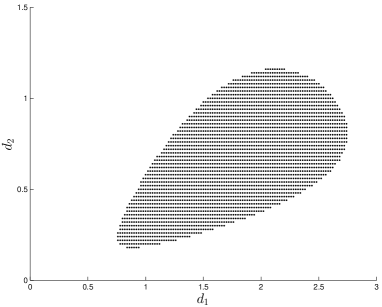
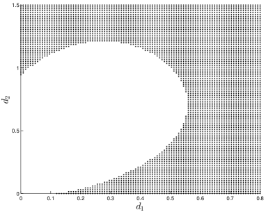
The stability results are depicted in Fig. 4, Fig. 5 and Fig. 6, respectively, where the shaded areas are the stability regions. In Case 1, the subsystems are chosen to be stable, the stability test result in Fig. 4 shows that the stability region is a non-convex set and that increasing the fixed dwell time (either $d_{1}$ or $d_{2}$ or both) will stabilize the system. This result suggests that slow switching is recommended when all the subsystems are stable. Case 2 corresponds to the situation where one subsystem is stable and the other is unstable; here $A_{1}$ is stable and $A_{2}$ unstable; the stability test result in Fig. 5 shows that the stable and unstable regions divide the first orthant into two semi-infinite parts, and the boundary between the two regions looks like a straight line. The result also confirms our expectation: increasing the dwell time in the stable subsystem will stabilize the system and increasing the dwell time in the unstable subsystem will destabilize it. In Case 3, the two subsystems are unstable. The test result in Fig. 6 shows that the stability region looks like a closed convex set and that both slow and fast switching will destabilize the system. Therefore, the dwell time needs to be chosen carefully to make the system stable in this case.

Finally, there are totally six variables in the computations of this example. The computational complexity is the same as the stability test for Markovian jump linear systems.

V Conclusions

This paper studied the stability property of randomly switched systems where the dwell time in each subsystem consists of a fixed part and a random part. We first showed the stochastic stability of such systems is equivalent to the stochastic stability of a class of Markovian jump systems with state jumps at the mode switching times. Then a necessary and sufficient condition for the system stability was derived using a stochastic Lyapunov approach. Finally, a numerical example was used to illustrate the application of the theory, and the results are consistent with our intuitions. Future research could be directed to the development of numerical algorithms to find the stabilizing switching parameters for the switched systems, and to the stability analysis of randomly switched singular systems, randomly switched 2D systems, randomly switched time-delay systems.

We provide two lemmas that are used in the proof of Lemma 1.

Lemma 2

Given a matrix $A\in\mathbb{R}^{n\times n}$, any vector $x\in\mathbb{R}^{n}$. Then there exists a constant $c_{0}\in\mathbb{R}$, which is independent of $x$, such that $\left\lVert e^{At}x\right\rVert^{2}\geq e^{c_{0}t}\left\lVert x\right\rVert^{2}$ for any $t\in[0,\infty)$. Moreover, given any $c\in(-\infty,c_{0}]$, $\left\lVert e^{At}x\right\rVert^{2}\geq e^{ct}\left\lVert x\right\rVert^{2}$ for $t\in[0,\infty)$.

Proof:

Let $c_{0}=\lambda_{\mathrm{min}}(A+A^{T})$. Then $A+A^{T}-c_{0}I\geq 0$. Consider the function $g(t)\triangleq\left\lVert e^{(A-\frac{c_{0}}{2}I)t}x\right\rVert^{2}$, we have

$$\frac{dg(t)}{dt} =\frac{d}{dt}\left\{x^{T}e^{(A-\frac{c_{0}}{2}I)^{T}t}e^{(A-\frac{c_{0}}{2}I)t}x\right\}$$

$$=x^{T}e^{(A^{T}-\frac{c_{0}}{2}I)t}\left[A+A^{T}-c_{0}I\right]e^{(A-\frac{c_{0}}{2}I)t}x$$

$$\geq 0$$

Hence $g(t)\geq g(0)$ for $t\in[0,\infty)$; that is, $\left\lVert e^{(A-\frac{c_{0}}{2}I)t}x\right\rVert^{2}\geq\left\lVert x\right\rVert^{2}$. Therefore, $\left\lVert e^{At}x\right\rVert^{2}=\left\lVert e^{(A-\frac{c_{0}}{2}I)t}e^{\frac{c_{0}}{2}It}x\right\rVert^{2}\geq e^{c_{0}t}\left\lVert x\right\rVert^{2}\geq e^{ct}\left\lVert x\right\rVert^{2}$ for any $t\in[0,\infty)$ and any $c\leq c_{0}$. ∎

Lemma 3

Given an exponentially distributed random variable $X$ with parameter $\lambda$, and two real numbers $a<\lambda$ and $b\in\mathbb{R}$. Then $\operatorname{E}\left\{\int_{b}^{b+X}e^{at}dt\right\}=\frac{e^{\lambda b}}{\lambda-a}$.

Proof:

The result follows from direct computation. That is,

$$\quad\operatorname{E}\left\{\int_{b}^{b+X}e^{at}dt\right\}\triangleq\int_{0}^{\infty}\left[\int_{b}^{b+x}e^{at}dt\right]\lambda e^{-\lambda x}dx$$

$$=\int_{b}^{\infty}\left[\int_{t-b}^{\infty}\lambda e^{-\lambda x}dx\right]e^{at}dt=\int_{b}^{\infty}e^{-\lambda(t-b)}e^{at}dt$$

$$=e^{\lambda b}\int_{0}^{\infty}e^{(a-\lambda)t}dt=\frac{e^{\lambda b}}{\lambda-a}$$

∎

Figure 4: Case 1: stability region of a switched system composed of two stable subsystems. The shaded area is the stability region. It shows that slow switching is recommended in this case.

Figure 5: Case 2: stability region of a switched system composed of a stable subsystem and an unstable subsystem. The shaded area is the stability region. It shows that increasing the dwell time in the stable subsystem will stabilize the system.

Figure 6: Case 3: stability region of a switched system composed of two unstable systems. The shaded area is the stability region. It shows that either slow or fast switching can destabilize the system and that a careful chosen dwell times can stabilize the system.

References

• [1] G. Wang, Y. Liu, C. Wen, and W. Chen, “Delay-dependent stability criterion and Hsubscript𝐻H_{\infty} state-feedback control for uncertain discrete-time switched systems with time-varying delays,” International Journal of Innovative Computing, Information and Control, vol. 7, no. 5(A), pp. 2473–2484, 2011.
• [2] H. R. Shaker and R. Wisniewski, “Model reduction of switched systems based on switching generalized gramians,” International Journal of Innovative Computing, Information and Control, vol. 8, no. 7(B), pp. 5025–5044, 2012.
• [3] C. Jiang, K. L. Teo, R. Loxton, and G.-R. Duan, “A neighboring extremal solution for optimal switched impulsive control problems with large perturbations,” International Journal of Innovative Computing, Information and Control, vol. 8, no. 9, pp. 6235–6257, 2012.
• [4] G. Zhang, C. Han, Y. Guan, and L. Wu, “Exponential stability analysis and stabilization of discrete-time nonlinear switched systems with time delays,” International Journal of Innovative Computing, Information and Control, vol. 8, no. 3(A), pp. 1973–1986, 2012.
• [5] J. P. Hespanha, “A model for stochastic hybrid systems with application to communication networks,” Nonlinear Analysis, vol. 62, no. 8, pp. 1353–1383, 2005.
• [6] E.-K. Boukas, Stochastic Switching Systems: Analysis and Design, W. S. Levine, Ed.   Birkhäuser, 2006.
• [7] R. Yang, P. Shi, G.-P. Liu, and H. Gao, “Network-based feedback control for systems with mixed delays based on quantization and dropout compensation,” Automatica, vol. 47, no. 12, pp. 2805–2809, 2011.
• [8] Q. Lu, L. Zhang, M. Basin, and H. Tian, “Analysis and synthesis for networked control systems with uncertain rate of packet losses,” Journal of the Franklin Institute, vol. 349, no. 7, pp. 2500–2514, 2012.
• [9] L. Zhang, H. Gao, and O. Kaynak, “Network-induced constraints in networked control systems—a survey,” IEEE Tansactions on Industrial Informatics, vol. 9, no. 1, pp. 403–416, 2013.
• [10] D. Liberzon, Switching in Systems and Control.   Birkhäuser, 2003.
• [11] X. Mao and C. Yuan, Stochastic Differential Equations with Markovian Switching.   Imperial College Press, 2006.
• [12] H. Lin and P. J. Antsaklis, “Stability and stabilizability of switched linear systems: a survey of recent results,” IEEE Transactions on Automatic Control, vol. 54, no. 2, pp. 308–322, 2009.
• [13] L. Wu, X. Su, and P. Shi, “Sliding mode control with bounded L2subscript𝐿2L_{2} gain performance of Markovian jump singular time-delay systems,” Automatica, vol. 48, no. 8, pp. 1929–1933, 2012.
• [14] L. Wu, P. Shi, H. Gao, and C. Wang, “Hsubscript𝐻H_{\infty} filtering for 2D Markovian jump systems,” Automatica, vol. 44, no. 7, pp. 1849–1858, 2008.
• [15] P. Shi, E.-K. Boukas, and R. K. Agarwal, “Control of Markovian jump discrete-time systems with norm bounded uncertainty and unknown delay,” IEEE Transactions on Automatic Control, vol. 44, no. 11, pp. 2139–2144, 1999.
• [16] J. Xiong, J. Lam, H. Gao, and D. W. C. Ho, “On robust stabilization of Markovian jump systems with uncertain switching probabilities,” Automatica, vol. 41, no. 5, pp. 897–903, 2005.
• [17] L. Zhang and J. Lam, “Necessary and sufficient conditions for analysis and synthesis of Markov jump linear systems with incomplete transition descriptions,” IEEE Transactions on Automatic Control, vol. 55, no. 7, pp. 1695–1701, 2010.
• [18] Y. Zhang, Y. He, M. Yu, and J. Zhang, “Stabilization for Markovian jump systems with partial information on transition probability based on free-connection weighting matrices,” Automatica, vol. 47, no. 1, pp. 79–84, 2011.
• [19] A. S. Morse, “Supervisory control of families of linear set-point controllers—part 1: exact matching,” IEEE Transactions on Automatic Control, vol. 41, no. 10, pp. 1413–1431, 1996.
• [20] Y. Ji and H. J. Chizeck, “Controllability, stabilizability, and continuous-time Markovian jump linear quadratic control,” IEEE Transactions on Automatic Control, vol. 35, no. 7, pp. 777–788, 1990.
• [21] B. Øksendal, Stochastic Differential Equations: An Introduction with Applications, 6th ed.   Springer-Verlag, 2005.
Refer to caption