Improved Submatrix Maximum Queries in Monge Matrices

Abstract

We present efficient data structures for submatrix maximum queries in Monge matrices and Monge partial matrices. For $n\times n$ Monge matrices, we give a data structure that requires $O(n)$ space and answers submatrix maximum queries in $O(\log n)$ time. The best previous data structure [Kaplan et al., SODA‘12] required $O(n\log n)$ space and $O(\log^{2}n)$ query time. We also give an alternative data structure with constant query-time and $O(n^{1+\varepsilon})$ construction time and space for any fixed $\varepsilon<1$. For $n\times n$ partial Monge matrices we obtain a data structure with $O(n)$ space and $O(\log n\cdot\alpha(n))$ query time. The data structure of Kaplan et al. required $O(n\log n\cdot\alpha(n))$ space and $O(\log^{2}n)$ query time.

Our improvements are enabled by a technique for exploiting the structure of the upper envelope of Monge matrices to efficiently report column maxima in skewed rectangular Monge matrices. We hope this technique will be useful in obtaining faster search algorithms in Monge partial matrices. In addition, we give a linear upper bound on the number of breakpoints in the upper envelope of a Monge partial matrix. This shows that the inverse Ackermann $\alpha(n)$ factor in the analysis of the data structure of Kaplan et. al is superfluous.

1 Introduction

A matrix $M$ is a Monge matrix if for any pair of rows $i<j$ and columns $k<\ell$ we have that $M_{ik}+M_{j\ell}\geq M_{i\ell}+M_{jk}$. Monge matrices have many applications in combinatorial optimization and computational geometry. For example, they arise in problems involving distances in the plane [20, 24, 26, 28], and in problems on convex $n$-gons [2, 3]. See [9] for a survey on Monge matrices and their uses in combinatorial optimization.

In this paper we consider the following problem: Given an $n\times n$ Monge matrix $M$, construct a data structure that can report the maximum entry in any query submatrix (defined by a set of consecutive rows and a set of consecutive columns). Recently, Kaplan, Mozes, Nussbaum and Sharir [21] presented an $\tilde{O}(n)$ space data structure with $\tilde{O}(n)$ construction time and $O(\log^{2}n)$ query time. They also described an extension of the data structure to handle partial Monge matrices (where some of the entries of $M$ are undefined, but the defined entries in each row and in each column are contiguous). The extended data structure incurs larger polylogarithmic factors in the space and construction time. Both the original and the extended data structures have various important applications. They are used in algorithms that efficiently find the largest empty rectangle containing a query point, in dynamic distance oracles for planar graphs, and in algorithms for maximum flow in planar graphs [6]. See [21] for more details on the history of this problem and its applications.

Note that, even though explicitly representing the input matrix requires $N=\Theta(n^{2})$ space, the additional space required by the submatrix maximum data structure of [21] is only $\tilde{O}(n)$. In many applications (in particular [6, 21]), the matrix $M$ is not stored explicitly but any entry of $M$ can be computed when needed in $O(1)$ time. The space required by the application is therefore dominated by the size of the submatrix maximum data structure. With the increasing size of problem instances, and with current memory and cache architectures, space often becomes the most significant resource.

For general (i.e., not Monge) matrices, a long line of research over the last three decades including [5, 13, 14, 17, 29] achieved $\tilde{O}(N)$ space and $\tilde{O}(1)$ query data structures, culminating with the $O(N)$-space $O(1)$-query data structure of Yuan and Atallah [29]. Here $N=n^{2}$ denotes the total number of entries in the matrix. It is also known [8] that reducing the space to $O(N/c)$ incurs an $\Omega(c)$ query-time. Tradeoffs requiring $O(N/c)$ additional space and $\tilde{O}(c)$ query-time were given in [7, 8]. When the matrix has only $N=o(n^{2})$ nonzero entries, the problem is known in computational geometry as the orthogonal range searching problem on the $n\times n$ grid. In this case as well, various tradeoffs with $\tilde{O}(N)$-space and $\tilde{O}(1)$-query appear in a long history of results including  [4, 10, 11, 15, 17]. In particular, a linear $O(N)$-space data structure was given by Chazelle [11] at the cost of an $O(\log^{\varepsilon}n)$ query time. See [25] for a survey on orthogonal range search.

Contribution.

Our first contribution is in designing $O(n)$-space $O(\log n)$-query data structures for submatrix maximum queries in Monge matrices and in partial Monge matrices (see Section 3). Our data structures improve upon the data structures of Kaplan et al. in both space and query time. Consequently, using our data structures for finding the largest empty rectangle containing a query point improves the space and query time by logarithmic factors.

We further provide alternative data structures with faster query-time; We achieve $O(1)$ query-time at the cost of $O(n^{1+\varepsilon})$ construction time and space for an arbitrarily small constant $0<\varepsilon<1$ (see Section 5).

Our results are achieved by devising a data structure for reporting column maxima in $m\times n$ Monge matrices with many more columns than rows ($n>>m$). We refer to this data structure as the micro data structure. The space required by the micro data structure is linear in $m$, and independent of $n$. Its construction-time depends only logarithmically on $n$. The query-time is $O(\log\log n)$, the time required for a predecessor query in a set of integers bounded by $n$. We use the micro data structure in the design of our submatrix maximum query data structures, exploiting its sublinear dependency on $n$, and an ability to trade off construction and query times.

For partial Monge matrices, we provide a tight $O(m)$ upper bound on the complexity of the upper envelope (see Section 4). The best previously known bound [27] was $m\alpha(m)$, where $\alpha(m)$ is the inverse Ackermann function. This upper bound immediately implies that the $\alpha(m)$ factor stated in the space and construction time of the data structures of Kaplan et al. is superfluous.

Notice that the upper envelope of a full $m\times n$ Monge matrix also has complexity $O(m)$. The famous SMAWK algorithm [2] can find all column maxima in $O(n+m)$ time. However, this is not the case for partial Monge matrices. Even for simple partial Monge matrices such as triangular, or staircase matrices, where it has been known for a long time that the complexity of the upper envelope is linear, the fastest known algorithm for finding all column maxima is the $O(n\alpha(m)+m)$ time algorithm of Klawe and Kleitman [22]. We hope that our micro data structure will prove useful for obtaining a linear-time algorithm. The known algorithms, including the $(n\alpha(m)+m)$-time algorithm of Klawe and Kleitman [22], partition the matrix into skewed rectangular matrices, and use the SMAWK algorithm. It is plausible that our micro data structure will yield a speed up since it is adapted to skewed matrices.

2 Preliminaries and Our Results

In this section we overview the data structures of [21] and highlight our results.

A matrix $M$ is a Monge matrix if for any pair of rows $i<j$ and columns $k<\ell$ we have that $M_{ik}+M_{j\ell}\geq M_{i\ell}+M_{jk}$. A matrix $M$ is totally monotone in columns if for any pair of rows $i<j$ and columns $k<\ell$ we have that if $M_{ik}\leq M_{jk}$ then $M_{i\ell}\leq M_{j\ell}$. Similarly, $M$ is totally monotone in rows if for any pair of rows $i<j$ and columns $k<\ell$ we have that if $M_{ik}\leq M_{i\ell}$ then $M_{jk}\leq M_{j\ell}$. Notice that the Monge property implies total monotonicity (in columns and in rows) but the converse is not true. When we simply say totally monotone (or TM) we mean totally monotone in columns (our results symmetrically apply to totally monotone in rows).

A matrix $M$ is a partial matrix if some entries of $M$ are undefined, but the defined entries in each row and in each column are contiguous. We assume w.l.o.g. that every row has at least one defined element and that the defined elements form a single connected component (i.e., the defined column intervals in each pair of consecutive rows overlap). If this is not the case then only minor changes are needed in our algorithms. A partial TM (resp., Monge) matrix is a partial matrix whose defined entries satisfy the TM (resp., Monge) condition.

The following propositions are easy to verify:

Proposition 1

An $m\times n$ matrix $M$ is Monge iff $M_{i,j}+M_{i+1,j+1}\geq M_{i+1,j}+M_{i,j+1}$ for all $i=1,2,\ldots,m-1$ and $j=1,2,\ldots,n-1$.

Proposition 2

If a matrix $M$ is partial Monge, then it remains partial Monge after replacing any element of $M$ by a blank, so long as the defined (non-blank) entries in each row and in each column remain contiguous.

Proposition 3

If an $m$-by-$n$ matrix $M$ is (partial) Monge, then the $(m+1)$-by-$n$ matrix resulting by replacing any row of $M$ by two identical copies of that row is also (partial) Monge. An analogous statement holds for duplicating any column of $M$.

We consider $m\times n$ matrices, but for simplicity we sometimes state the results for $n\times n$ matrices. For a Monge matrix $M$, denote $r(j)=i$ if the maximum element in column $j$ lies in row $i$. (We assume this maximum element is unique. It is simple to break ties by, say, taking the highest index.) The upper envelope $\mathcal{E}$ of all the rows of $M$ consists of the $n$ values $r(1),\ldots,r(n)$. Since $M$ is Monge we have that $r(1)\leq r(2)\leq\ldots\leq r(n)$ and so $\mathcal{E}$ can be implicitly represented in $O(m)$ space by keeping only the $r(j)$s of $O(m)$ columns called breakpoints. Breakpoints are the columns $j$ where $r(j)\neq r(j+1)$. The maximum element $r(\pi)$ of any column $\pi$ can then be retrieved in $O(\log m)$ time by a binary search for the first breakpoint-column $j$ after $\pi$, and setting $r(\pi)=r(j)$.

The first data structure of [21] is a balanced binary tree $T_{h}$ over the rows of $M$. A node $u$ whose subtree contains $k$ leaves (i.e., $k$ rows) stores the $O(k)$ breakpoints of the $k\times n$ matrix $M^{u}$ defined by these $k$ rows and all columns of $M$. A leaf represents a single row and requires no computation. An internal node $u$ obtains its breakpoints by merging the breakpoints of its two children: its left child $u_{1}$ and its right $u_{2}$. By the Monge property, the list of breakpoints of $u$ starts with a prefix of breakpoints of $u_{1}$ and ends with a suffix of breakpoints of $u_{2}$. Between these there is possibly one new breakpoint $j$. The prefix and suffix parts can be found easily in $O(k)$ time by linearly comparing the lists of breakpoints of $u_{1}$ and $u_{2}$. The new breakpoint $j$ can then be found in additional $O(\log n)$ time via binary search. Summing $O(k+\log n)$ over all nodes of $T_{h}$ gives $O(m(\log m+\log n))$ time. The total size of $T_{h}$ is $O(m\log m)$.

Note that the above holds even if $M$ is not Monge but only TM. This gives rise to a data structure that answers subcolumn (as opposed to submatrix) queries:

Subcolumn queries in TM matrices [21]. Given a $n\times n$ TM matrix, one can construct, in $O(n\log n)$ time, a data structure of size $O(n\log n)$ that reports the maximum in a query column and a contiguous range of rows in $O(\log n)$ time.

The maximum entry in a query column $\pi$ and a contiguous range of rows $R$ is found using $T_{h}$ by identifying $O(\log m)$ canonical nodes of $T_{h}$. A node $u$ is canonical if $u$’s set of rows is contained in $R$ but the set of rows of $u$’s parent is not. For each such canonical node $u$, we find in $O(\log m)$ time the maximum element in column $\pi$ amongst all the rows of $u$. The output is the largest of these and the total query time is $O(\log^{2}m)$. The query time can be reduced to $O(\log m)$ by using fractional cascading [12].

The first results of our paper improve the above subcolumn query data structure of [21], as indicated in Table 1 under subcolumn query in TM matrices. The next data structure of [21] extends the queries from subcolumn to submatrix (specified by ranges $R$ of consecutive rows, and $C$ of consecutive columns.)

Submatrix queries in Monge matrices [21]. Given a $n\times n$ Monge matrix, one can construct, in $O(n\log n)$ time, a data structure of size $O(n\log n)$ that reports the maximum entry in a query submatrix in $O(\log^{2}n))$ time.

To obtain $O(\log^{2}n)=O(\log m(\log m+\log n))$ query time, note that $R$ is the disjoint union of $O(\log m)$ canonical nodes of $T_{h}$. For each such canonical node $u$, we use $u$’s list of breakpoints $\{j_{1},j_{2},\ldots,j_{k}\}$ to find in $O(\log m+\log n)$ time the maximum element in all rows of $u$ and the range of columns $C$. This is done as follows: we first identify in $O(\log m)$ time the set $\mathcal{I}=\{j_{a},j_{a+1},\ldots,j_{b}\}$ of $u$’s breakpoints that are fully contained in $C$. The columns of $C$ that are to the left of $j_{a}$ all have their maximum element in row $r(j_{a})$. To find the maximum of these we construct, in addition to $T_{h}$, a symmetric binary tree $\mathcal{B}$ that can report in $O(\log n)$ time the maximum entry in a query row and a contiguous range of columns. $\mathcal{B}$ is built in $O(n(\log m+\log n))$ time and $O(n\log n)$ space using the subcolumn query data structure on the transpose of $M$. This is possible since $M$ is Monge. Similarly, we find in $O(\log n)$ time the maximum in all columns of $C$ that are to the right of $j_{b}$.

To find the maximum in all columns between $j_{a}$ and $j_{b}$, let $m(j_{i})$ denote the maximum element in the columns interval $(j_{i-1},j_{i}]$ (note it must be in row $r(j_{i})$). We wish to find $\max\{m(j_{a+1}),\ldots,m(j_{b})\}$ which corresponds to a Range Maximum Query in the array $A^{u}=\{m(j_{1}),\ldots,m(j_{k})\}$. We compute the array $A^{u}$ (along with a naive RMQ data structure with logarithmic query time) of every node $u$ during the construction of $T_{h}$. Most of the entries of $A^{u}$ are simply copied from $u$’s children arrays $A^{u_{1}}$ and $A^{u_{2}}$. The only new $m(\cdot)$ value that $u$ needs to compute is for the single new breakpoint $j$ (that is between the prefix from $u_{1}$ and the suffix from $u_{2}$). Since $m(j)$ must be in row $r(j)$ it can be computed in $O(\log n)$ time by a single query to $\mathcal{B}$.

Overall, we get a query time of $O(\log m+\log n)$ per canonical node $u$ for a total of $O(\log m(\log m+\log n))$. Building $T_{h}$ (along with all the RMQ arrays $A^{u}$) and $\mathcal{B}$ takes total $O((m+n)(\log m+\log n))$ time and $O(m\log m+n\log n)$ space. Our two improvements to this bound of [21] are stated in Table 1 under submatrix queries in Monge matrices.

The next data structures of [21] extend the above subcolumn and submatrix data structures from full to partial TM matrices. The construction is very similar. Merging the breakpoints of the two children $u_{1}$, $u_{2}$ of a node $u$ of $T_{h}$ is slightly more involved now, since the envelopes may cross each other multiple times. The number of breakpoints of any subset of consecutive $k$ rows is $O(k\cdot\alpha(k))$ [27], and so there are $O(m\log m\cdot\alpha(m))$ breakpoints in total over all nodes of $T_{h}$ (as opposed to $O(m)$ in full matrices). This implies the following

Subcolumn queries in partial TM matrices [21]. Given a partial TM $n\times n$ matrix, one can construct, in $O(n\log^{2}n\cdot\alpha(n))$ time, a data structure of size $O(n\log n\cdot\alpha(n))$ that reports the maximum entry in a query column and a contiguous range of rows in $O(\log n)$ time.

We improve this data structure to the same bounds we get for full matrices. i.e, we show that our bounds for full matrices also apply to partial matrices. This is stated in Table 1 under subcolumn query in Partial TM matrices. Finally, [21] extended their submatrix data structure from full to partial Monge matrices. It uses a similar construction of $T_{h}$ and $\mathcal{B}$ as in the case of full matrices, but again requires the additional $O(\log m\cdot\alpha(m)+\log n\cdot\alpha(n))$ multiplicative factor to store the breakpoints of all nodes of $T_{h}$ and $\mathcal{B}$.

property	query type	space	construction time	query time
TM	subcolumn	$O(n\log n)$	$O(n\log n)$	$O(\log n)$	Lemma 3.1 in [21]
TM	subcolumn	$O(n)$	$O(n\log n/\log\log n)$	$O(\log n)$	Lemma 2 here
TM	subcolumn	$O(n^{1+\varepsilon})$	$O(n^{1+\varepsilon})$	$O(1)$	Lemma 8 here
Monge	submatrix	$O(n\log n)$	$O(n\log n)$	$O(\log^{2}n)$	Theorem 3.2 in [21]
Monge	submatrix	$O(n)$	$O(n\log n)$	$O(\log n)$	Theorem 3.1 here
Monge	submatrix	$O(n)$	$O(n\log n/\log\log n)$	$O(\log^{1+\varepsilon}n)$	Corollary 1 here
Monge	submatrix	$O(n^{1+\varepsilon})$	$O(n^{1+\varepsilon})$	$O(1)$	Theorem 5.1 here
Partial TM	subcolumn	$O(n\log n\cdot\alpha(n))$	$O(n\log^{2}n\cdot\alpha(n))$	$O(\log n)$	Lemma 3.3 in [21]
Partial TM	subcolumn	$O(n)$	$O(n\log n/\log\log n)$	$O(\log n)$	Lemma 3 here
Partial TM	subcolumn	$O(n^{1+\varepsilon})$	$O(n^{1+\varepsilon})$	$O(1)$	Lemma 3 here
Partial Monge	submatrix	$O(n\log n\cdot\alpha(n))$	$O(n\log^{2}n\cdot\alpha(n))$	$O(\log^{2}n)$	Theorem 3.4 in [21]
Partial Monge	submatrix	$O(n)$	$O(n\log n)$	$O(\log n\cdot\alpha(n))$	Theorem 3.2 here
Partial Monge	submatrix	$O(n)$	$O(n\log n/\log\log n)$	$O(\log^{1+\varepsilon}n\cdot\alpha(n))$	Corollary 2 here

Table 1: Our results compared to [21].

Submatrix queries in partial Monge matrices [21]. Given a $n\times n$ partial Monge matrix, one can construct, in $O(n\alpha(n)\log^{2}n)$ time, a data structure of size $O(n\alpha(n)\log n)$ that reports the maximum entry in a query submatrix in $O(\log^{2}n)$ time.

We remove the $O(\log n\cdot\alpha(n))$ multiplicative factor and obtain the bounds stated in the bottom of Table 1. The $\alpha(n)$ factor is removed by showing that the number of breakpoints in the upper envelope of a partial Monge matrix is linear.

3 Linear-Space Data Structures

In this section we present our data structures that improve the space to $O(n)$ and the query time to $O(\log n)$. We begin by introducing a new data structure for the case where a query is composed of an entire column (as opposed to a range of rows). This new data structure (which we call the micro data structure) is designed to work well when the number of rows in the matrix is much smaller than the number of columns. We denote by $pred(x,n)=O(\min\{\log x,\log\log n\})$ the time to query a predecessor data structure with $x$ elements from $\{1,\ldots,n\}$.

Lemma 1 (the micro data structure)

Given a $x\times n$ TM matrix and $r>0$, one can construct in $O(x\log n/\log r)$ time, a data structure of size $O(x)$ that given a query column can report the maximum entry in the entire column in $O(r+pred(x,n))$ time.

Proof

Out of all $n$ columns of the input matrix $M$, we will designate $O(x)$ columns as special columns. For each of these special columns we will eventually compute its maximum element. The first $x$ special columns of $M$ are columns $1,n/x,2n/x,3n/x,\ldots,n$ and are denoted $j_{1},\ldots,j_{x}$.

Let $X$ denote the $x\times x$ submatrix obtained by taking all $x$ rows but only the $x$ special columns $j_{1},\ldots,j_{x}$. It is easy to verify that $X$ is TM. We can therefore run the SMAWK algorithm [2] on $X$ in $O(x)$ time and obtain the column maxima of all special columns. Let $r(j)$ denote the row containing the maximum element in column $j$. Since $M$ is TM, the $r(j)$ values are monotonically non-decreasing. Consequently, $r(j)$ of a non-special column $j$ must be between $r(j_{i})$ and $r(j_{i+1})$ where $j_{i}<j$ and $j_{i+1}>j$ are the two special columns bracketing $j$ (see Figure 1).

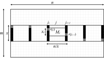
Figure 1: An $x\times n$ matrix inside an $m\times n$ matrix. The black columns are the first $x$ special columns. The (monotonically non-decreasing) gray cells inside these special columns are the column maxima (i.e., the $r(j_{i})$ values of breakpoints $j_{i}$). The maximum element of column $j$ in the $x\times n$ matrix must be between $r(j_{i})$ and $r(j_{i+1})$ (i.e., in matrix $M_{i}$).

For every $i$, let $x_{i}=r(j_{i+1})-r(j_{i})$. If $x_{i}\leq r$ then no column between $j_{i}$ and $j_{i+1}$ will ever be a special column. When we will query such a column $j$ we can simply check (at query-time) the $r$ elements of $j$ between rows $r(j_{i})$ and $r(j_{i+1})$ in $O(r)$ time. If, however, $x_{i}>r$, then we designate more special columns between $j_{i}$ and $j_{i+1}$. This is done recursively on the $x_{i}\times(n/x)$ matrix $M_{i}$ composed of rows $r(j_{i}),\ldots,r(j_{i+1})$ and columns $j_{i},\ldots,j_{i+1}$. That is, we mark $x_{i}$ evenly-spread columns of $M_{i}$ as special columns, and run SMAWK in $O(x_{i})$ time on the $x_{i}\times x_{i}$ submatrix $X_{i}$ obtained by taking all $x_{i}$ rows but only these $x_{i}$ special columns. We continue recursively until either $x_{i}\leq r$ or the number of columns in $M_{i}$ is at most $r$. In the latter case, before terminating, the recursive call runs SMAWK in $O(x_{i}+r)=O(x_{i})$ time on the $x_{i}\times r$ submatrix $X_{i}$ obtained by taking the $x_{i}$ rows and all columns of $M_{i}$ (i.e., all columns of $M_{i}$ will become special).

After the recursion terminates, every column $j$ of $M$ is either special (in which case we computed its maximum), or its maximum is known to be in one of at most $r$ rows (these rows are specified by the $r(\cdot)$ values of the two special columns bracketing $j$). Let $s$ denote the total number of columns that are marked as special. We claim that $s=O(x\log n/\log r)$. To see this, notice that the number of columns in every recursive call decreases by a factor of at least $r$ and so the recursion depth is $O(\log_{r}n)=O(\log n/\log r)$. In every recursive level, the number of added special columns is $\sum x_{i}$ over all $x_{i}^{\prime}s$ in this level that are at least $r$. In every recursive level, this sum is bounded by $2x$ because each one of the $x$ rows of $M$ can appear in at most two $M_{i}$’s (as the last row of one and the first row of the other). Overall, we get $2x\cdot O(\log n/\log r)=O(x\log n/\log r)$.

Notice that $s=O(x\log n/\log r)$ implies that the total time complexity of the above procedure is also $O(x\log n/\log r)$. This is because whenever we run SMAWK on a $y\times y$ matrix it takes $O(y)$ time and $y$ new columns are marked as special. To complete the construction, we go over the $s$ special columns from left to right in $O(s)$ time and throw away (mark as non-special) any column whose $r(\cdot)$ value is the same as that of the preceding special column. This way we are left with only $O(x)$ special columns, and the difference in $r(\cdot)$ between consecutive special columns is at least $1$ and at most $r$. In fact, it is easy to maintain $O(x)$ (and not $O(s)$) space during the construction by only recursing on sub matrices $M_{i}$ where $x_{i}>1$. We note that when $r=1$, the eventual special columns are exactly the set of breakpoints of the input matrix $M$.

The final data structure is a predecessor data structure that holds the $O(x)$ special columns and their associated $r(\cdot)$ values. Upon query of some column $j$, we search in $pred(x,n)$ time for the predecessor and successor of $j$ and obtain the two $r(\cdot)$ values. We then search for the maximum of column $j$ by explicitly checking all the (at most $r$) relevant rows of column $j$. The query time is therefore $O(r+pred(x,n))$ and the space $O(x)$. ∎

A linear-space subcolumn data structure.

Lemma 2

Given a $m\times n$ TM matrix, one can construct, in $O(m(\log n+\log m)/\log\log m)$ time, a data structure of size $O(m)$ that can report the maximum entry in a query column and a contiguous range of rows in $O(\log m)$ time.

Proof

Given an $m\times n$ input matrix $M$ we partition it into $m/x$ matrices $M^{1},M^{2},\ldots,M^{m/x}$ where $x=\log m$. Every $M^{i}$ is an $x\times n$ matrix composed of $x$ consecutive rows of $M$. We construct the micro data structure of Lemma 1 for each $M^{i}$ separately choosing $r=x^{\varepsilon}$ for any constant $0\!<\!\varepsilon\!<\!1$. This requires $O(x\log n/\log r)=O(x\log n/\log x)$ construction time per $M^{i}$ for a total of $O(m\log n/\log\log m)$ time. We obtain a (micro) data structure of total size $O(m)$ that upon query $(i,j)$ can report in $O(x^{\varepsilon}+pred(x,n))=O(\log^{\varepsilon}m)$ time the maximum entry in column $j$ of $M^{i}$.

Now, consider the $(m/x)\times n$ matrix $M^{\prime}$, where $M^{\prime}_{ij}$ is the maximum entry in column $j$ of $M^{i}$. We cannot afford to store $M^{\prime}$ explicitly, however, using the micro data structure we can retrieve any entry $M^{\prime}_{ij}$ in $O(\log^{\varepsilon}m)$ time. We next show that $M^{\prime}$ is also TM.

For any pair of rows $i<j$ and any pair of columns $k<\ell$ we need to show that if $M^{\prime}_{ik}\leq M^{\prime}_{jk}$ then $M^{\prime}_{i\ell}\leq M^{\prime}_{j\ell}$. Suppose that $M^{\prime}_{ik},M^{\prime}_{jk},M^{\prime}_{i\ell}$, and $M^{\prime}_{j\ell}$ correspond to entries $M_{ak},M_{bk},M_{c\ell}$, and $M_{d\ell}$ respectively. We assume that $M_{ak}\leq M_{bk}$ and we need to show that $M_{c\ell}\leq M_{d\ell}$. Notice that $M_{ck}\leq M_{ak}$ because $M_{ak}$ is the maximal entry in column $k$ of $M^{i}$ and $M_{ck}$ is also an entry in column $k$ of $M^{i}$. Since $M_{ck}\leq M_{ak}$ and $M_{ak}\leq M_{bk}$ we have that $M_{ck}\leq M_{bk}$. Since $M_{ck}\leq M_{bk}$, from the total monotonicity of $M$, we have that $M_{c\ell}\leq M_{b\ell}$. Finally, we have $M_{b\ell}\leq M_{d\ell}$ because $M_{d\ell}$ is the maximal entry in column $\ell$ of $M^{j}$ and $M_{b\ell}$ is also an entry in column $\ell$ of $M^{j}$. We conclude that $M_{c\ell}\leq M_{d\ell}$.

Now that we have established that the matrix $M^{\prime}$ is TM, we can use the subcolumn data structure of [21] (see previous section) on $M^{\prime}$. Whenever an entry $M^{\prime}_{ij}$ is desired, we can retrieve it using the micro data structure. This gives us the macro data structure: it is of size $O(m/x\cdot\log(m/x))=O(m)$ and can report in $O(\log m)$ time the maximum entry of $M^{\prime}$ in a query column and a contiguous range of rows. It is built in $O(m/x\cdot(\log(m/x)+\log n)\cdot x^{\varepsilon})$ time which is $O(m(\log n+\log m)/\log\log m)$ for any choice of $\varepsilon<1$.

To complete the proof of Lemma 2 we need to show how to answer a general query in $O(\log m)$ time. Recall that a query is composed of a column of $M$ and a contiguous range of rows. If the range is smaller than $\log m$ we can simply check all elements explicitly in $O(\log m)$ time and return the maximum one. Otherwise, the range is composed of three parts: a prefix part of length at most $\log m$, an infix part that corresponds to a range in $M^{\prime}$, and a suffix part of length at most $\log m$. The prefix and suffix are computed explicitly in $O(\log m)$ time. The infix is computed by querying the macro data structure in $O(\log m)$ time. ∎

A linear-space submatrix data structure.

Theorem 3.1

Given a $m\times n$ Monge matrix, one can construct, in $O((m+n)(\log n+\log m))$ time, a data structure of size $O(m+n)$ that can report the maximum entry in a query submatrix in $O(\log m+\log n)$ time.

Proof

Recall from Section 2 that the submatrix data structure of [21] is composed of the tree $T_{h}$ over the rows of $M$ and the tree $\mathcal{B}$ over the columns of $M$. Every node $u\in T_{h}$ stores its breakpoints along with the RMQ array $A^{u}$ (where $A^{u}[j]$ holds the value of the maximum element between the $(j-1)$’th and the $j$’th breakpoints of $u$). If $u$ has $k$ breakpoints then they are computed along with $A^{u}$ in $O(k+\log n)$ time: $O(k)$ to copy from the children of $u$ and $O(\log n)$ to find the new breakpoint and to query $\mathcal{B}$. As opposed to [21], we don’t use a naive RMQ data structure but instead one of the existing linear-construction constant-query RMQ data structures such as [19].

To prove Theorem 3.1 we begin with two changes to the above. First, we build $T_{h}$ on the rows of the $(m/x)\times n$ matrix $M^{\prime}$ instead of the $m\times n$ matrix $M$ (again, when an entry $M^{\prime}_{ij}$ is desired, we retrieve it using the micro data structure in $O(x^{\varepsilon})$ time). Second, for $\mathcal{B}$ we use the data structure of Lemma 2 applied to the transpose of $M$. $\mathcal{B}$’s construction requires $O(n(\log m+\log n)/\log\log n)$ time and $O(n)$ space. After this, constructing $T_{h}$ (along with the $A_{u}$ arrays) on $M^{\prime}$ requires $O(m/x\cdot\log(m/x))=O(m)$ space and $O((m/x)(\log(m/x)+\log n)\cdot x^{\varepsilon})=O(m(\log m+\log n)/\log\log m)$ time by choosing $x=\log m$ and any $\varepsilon<1$.

Finally, we construct a data structure $T_{v}$ that is symmetric to $T_{h}$ but applied to the transpose of $M$. Notice that $T_{v}$ is built on the columns of an $m\times(n/\log n)$ matrix $M^{\prime\prime}$ instead of the $m\times n$ matrix $M$. The construction of $T_{v}$, from a symmetric argument to the previous paragraph, also takes $O((m+n)(\log n+\log m)/\log\log m)$ time and $O(m+n)$ space.

We now describe how to answer a submatrix query with row range $R$ and column range $C$. Let $R^{\prime}$ be the set of consecutive rows of $M^{\prime}$ whose corresponding rows in $M$ are entirely contained in $R$. Let $R_{p}$ be the prefix of $O(\log m)$ rows of $R$ that do not correspond to rows of $R^{\prime}$. Let $R_{s}$ be the suffix of $O(\log m)$ rows of $R$ that do not correspond to rows of $R^{\prime}$. We define the subranges $C^{\prime},C_{p},C_{s}$ similarly (with respect to columns and to $M^{\prime\prime}$). The submatrix query $(R,C)$ can be covered by the following: (1) a submatrix query $(R^{\prime},C)$ in $M^{\prime}$, (2) a submatrix query $(R,C^{\prime})$ in $M^{\prime\prime}$, and (3) four small $O(\log m)\times O(\log n)$ submatrix queries in $M$ for the ranges $(R_{i},C_{j})$, $i,j\in\{p,s\}$. We find the maximum in each of these six ranges and return the maximum of the six values.

We find the maximum of each of the small $O(\log m)\times O(\log n)$ ranges of $M$ in $O(\log m+\log n)$ time using the SMAWK algorithm. The maximum in the submatrix of $M^{\prime}$ is found using $T_{h}$ as follows (the maximum in the submatrix of $M^{\prime\prime}$ is found similarly using $T_{v}$). Notice that $R^{\prime}$ is the disjoint union of $O(\log m)$ canonical nodes of $T_{h}$. For each such canonical node $u$, we use binary-search on $u$’s list of breakpoints $\{j_{1},j_{2},\ldots,j_{k}\}$ to find the set $\{j_{a},j_{a+1},\ldots,j_{b}\}$ of $u$’s breakpoints that are fully contained in $C$. Although this binary-search can take $O(\log m)$ time for each canonical node, using fractional cascading, the searches on all canonical nodes take only $O(\log m)$ time and not $O(\log^{2}m)$. The maximum in all rows of $u$ and all columns between $j_{a}$ and $j_{b}$ is found by one query to the RMQ array $A^{u}$ in $O(1)$ time. Over all canonical nodes this takes $O(\log m)$ time.

The columns of $C$ that are to the left of $j_{a}$ all have their maximum element in row $r(j_{a})$ of $M^{\prime}$ (that is, in one of $O(\log m)$ rows of $M$) . Similarly, the columns of $C$ that are to the right of $j_{b}$ all have their maximum element in row $r(j_{b+1})$ of $M^{\prime}$. This means we have two rows of $M^{\prime}$, $r(j_{a})$ and $r(j_{b+1})$, where we need to search for the maximum. We do this only after we have handled all canonical nodes. That is, after we handle all canonical nodes we have a set $A=a_{1},a_{2},\dots$ of $2\log m$ rows of $M^{\prime}$ in which we still need to find the maximum. We apply the same procedure on $T_{v}$ which gives us a set $B=b_{1},b_{2},\dots$ of $2\log n$ columns of $M^{\prime\prime}$ in which we still have to find the maximum. Note that we only need to find the maximum among the elements of $M$ that lie in rows corresponding to a row in $A$ and in columns corresponding to a column in $B$. This amounts to finding the maximum of the $O(\log m)\times O(\log n)$ matrix $\bar{M}$, with $\bar{M}_{ij}$ being the maximum among the elements of $M$ in the intersection of the $x$ rows corresponding to row $a_{i}$ of $M^{\prime}$, and of the $x$ columns corresponding to column $b_{j}$ of $M^{\prime\prime}$.

An argument similar to the one in Lemma 2 shows that $\bar{M}$ is Monge. Therefore we can find its maximum element using the SMAWK algorithm. We claim that each element of $\bar{M}$ can be computed in $O(1)$ time, which implies that SMAWK finds the maximum of $\bar{M}$ in $O(x)$ time.

It remains to show how to compute an element of $\bar{M}$ in constant time. Recall from the proof of Lemma 2 that $M$ is partitioned into $x$-by-$n$ matrices $M^{i}$. During the preprocessing stage, for each $M^{i}$ we compute and store its upper envelope, and an RMQ array over the maximum elements in each interval of the envelope (similar to the array $A^{u}$). Computing the upper envelope takes $O(x\log n)$ time by incrementally adding one row at a time and using binary search to locate the new breakpoint contributed by the newly added row. Finding the maximum within each interval of the upper envelope can be done in $O(x\log n)$ time using the tree $\mathcal{B}$. We store the upper envelope in an atomic heap [16], which supports predecessor searches in constant time provided $x$ is $O(\log n)$. Overall the preprocessing time is $O(m\log n)$, and the space is $O(m)$. We repeat the same preprocessing on the transpose of $M$.

Now, given a row $a_{i}$ of $M^{\prime}$ and column $b_{j}$ of $M^{\prime\prime}$, let $[c_{a},c_{b}]$ be the range of $x$ columns of $M$ that correspond to $b_{j}$. We search in constant time for the successor $c_{a^{\prime}}$ of $c_{a}$ and for the predecessor $c_{b^{\prime}}$ of $c_{b}$ in the upper envelope of $M^{a_{i}}$. We use the RMQ array to find in $O(1)$ time the maximum element $y$ among elements in all rows of $M$ corresponding to $a_{i}$ and columns in the range $[c_{a^{\prime}},c_{b^{\prime}})$. The maximum element in columns $[c_{a},c_{a^{\prime}})$ and $[c_{b^{\prime}},c_{b}]$ is contributed by two known rows $r_{1},r_{2}$. We repeat the symmetric process for the transpose of $M$, obtaining a maximum element $y^{\prime}$, and two columns $c_{1},c_{2}$. $\bar{M}_{a_{i},b_{j}}$ is the maximum among six values: $y,y^{\prime}$ and the four elements $M_{r_{1}c_{1}},M_{r_{1}c_{2}},M_{r_{2}c_{1}},M_{r_{2}c_{2}}$. ∎

Notice that in the above proof, in order to obtain an element of $\bar{M}$ in constant time, we loose the $O(\log\log m)$ speedup in the construction time. This is because we found the upper envelope of each $M^{i}$. To get the $O(\log\log m)$ speedup we can obtain an element of $\bar{M}$ in $O(x^{\varepsilon})$ time using the micro data structure.

Corollary 1

Given a $m\times n$ Monge matrix, one can construct, in $O((m+n)(\log n+\log m)/\log\log m)$ time, a data structure of size $O(m+n)$ that reports the maximum entry in a query submatrix in $O((\log m+\log n)^{1+\varepsilon})$ time for any fixed $0<\varepsilon<1$.

A linear-space subcolumn data structure for partial matrices.

We next claim that the bounds of Lemma 2 for TM matrices also apply to partial TM matrices. The reason is that we can efficiently turn any partial TM matrix $M$ into a full TM matrix by implicitly filling appropriate constants instead of the blank entries.

Lemma 3

The blank entries in an $m\times n$ partial Monge matrix $M$ can be implicitly replaced in $O(m+n)$ time so that $M$ becomes Monge and each $M_{ij}$ can be returned in $O(1)$ time.

Proof

Let $s_{i}$ (resp. $t_{i}$) denote the index of the leftmost (resp. rightmost) column that is defined in row $i$. Since the defined (non-blank) entries of each row and column are continuous we have that the sequence $s_{1},s_{2},\ldots,s_{m}$ starts with a non-increasing prefix $s_{1}\geq s_{2}\geq\ldots\geq s_{a}$ and ends with a non-decreasing suffix $s_{a}\leq s_{a+1}\leq\ldots\leq s_{m}$. Similarly, the sequence $t_{1},t_{2},\ldots,t_{n}$ starts with a non-decreasing prefix $t_{1}\leq t_{2}\leq\ldots\leq t_{b}$ and ends with a non-increasing suffix $t_{b}\geq t_{b+1}\geq\ldots\geq t_{m}$.

We partition the blank region of $M$ into four regions: (I) entries that are above and to the left of $M[i,s_{i}]$ for $i=1,\ldots,a$, (II) entries that are below and to the left of $M[i,s_{i}]$ for $i=a+1,\ldots,m$, (III) entries that are above and to the right of $M[i,t_{i}]$ for $i=1,\ldots,b$, (IV) entries that are below and to the right of $M[i,t_{i}]$ for $i=b+1,\ldots,n$. We first describe how to replace all entries in region I to make them non-blank and obtain a valid partial Monge matrix (whose blank entries are only in regions II, III, and IV). The remaining regions are handled in a similar manner, one after the other.

We describe our method for filling in the blank entries in region I in two steps. In the first step we show how to implicitly fill in the blanks in a lower right triangular Monge matrix so that each filled blank entry can be computed in $O(1)$ time. By a lower right triangular Monge matrix we mean a partial Monge square matrix with $n$ rows and columns, such that, for all $1\leq i\leq n$, $s(i)=n-i+1$. In the second step we explain that any $m$-by-$n$ partial Monge matrix whose blank entries are in region I can be turned into a lower right triangular Monge matrix with at most $m+n$ rows and columns. The only operations used in the transformation are duplicating rows, duplicating columns, and turning elements into blanks. We will show an $O(m+n)$ procedure for computing two tables. One specifying, for each row index $1\leq i\leq m$, the corresponding row index in the larger $O(m+n)$ triangular matrix. The second is an analogous table for the columns indices. The lemma then follows for the blank entries in region I. The other regions are treated by reducing to the region I case, one after the other.

We now describe how to fill in the blank regions in a lower right triangular Monge matrix. Let $W$ denote the largest absolute value of any non-blank entry in $M$ (We can find $W$ by applying the algorithm of Klawe and Kleitman [23]). Intuitively, we would like to make every $M[i,j]$ in the upper left triangle very large. However, we cannot simply assign the same large value to all of them, because then the Monge inequality would not be guaranteed to hold if more than one of the four considered elements belongs to the replaced part of the matrix. A closer look at all possible cases shows that setting all the entries of each diagonal to the same value does work. More precisely, we replace the blank element $M[i,j]$ with $3W[2(n-i-j)+1]$. Thus, each element in the first diagonal off the main diagonal ($i+j=n$) is set to $3W$, the elements of the second diagonal off the main diagonal are set to $9W$, etc. Note that the maximum element in the resulting matrix is $O(nW)$. To prove that the resulting new matrix $M^{\prime}$ is Monge, it suffices, by Proposition 1, to show that, for all $1\leq i,k<n$, $M^{\prime}[i,k]+M^{\prime}[i+1,k+1]-M^{\prime}[i,k+1]-M^{\prime}[i+1,k]\geq 0$. To this end we consider the following cases:

1. $i+k>n$, so all $M[i,k],M[i+1,k+1],M[i,k+1],M[i+1,k]$ are non-blank, and the inequality holds because $M$ is partial Monge.

2. $i+k=n$, so $M[i,k]$ is blank and $M[i+1,k+1],M[i,k+1],M[i+1,k]$ are non-blank. Then
   $M^{\prime}[i,k]+M^{\prime}[i+1,k+1]-M^{\prime}[i,k+1]-M^{\prime}[i+1,k]=3W+M^{\prime}[i+1,k+1]-M^{\prime}[i,k+1]-M^{\prime}[i+1,k]\geq 3W-3W=0$.

3. $i+k=n-1$, so $M[i,k],M[i,k+1],M[i+1,k]$ are blank, and $M[i+1,k+1]$ is non blank. Then
   $M^{\prime}[i,k]+M^{\prime}[i+1,k+1]-M^{\prime}[i,k+1]-M^{\prime}[i+1,k]=9W+M[i+1,k+1]-3W-3W\geq 3W-W\geq 0$.

4. $i+k<n-1$, so all $M[i,k],M[i+1,k+1],M[i,k+1],M[i+1,k]$ are blank. Then,
   $M^{\prime}[i,k]+M^{\prime}[i+1,k+1]-M^{\prime}[i,k+1]-M^{\prime}[i+1,k]=0$.

Hence the new matrix $M^{\prime}$ is indeed Monge.

Next, we describe how to turn any $m$-by-$n$ partial Monge matrix $M$ whose blank entries are in region I into a slightly larger lower right triangular matrix $M^{\prime}$. This is done by duplicating rows or columns of $M$ and replacing by blanks a nonempty prefix in all but a single copy. Thus, each row $r$ (column $c$) of $M$ has exactly one appearance in $M^{\prime}$ in which no elements are replaced by blanks. We say that $r$ ($c$) is mapped to this appearance in $M^{\prime}$. Propositions 2 and 3 guarantee that $M^{\prime}$ is partial Monge. For ease of presentation we describe the process as if we actually transform the $M$ into $M^{\prime}$.

The assumption that the blank entries are in region I implies that $s_{1}\geq s_{2}\geq\cdots\geq s_{m}$ and that $t_{1}=t_{2}=\cdots=t_{m}$. We first guarantee that the $s_{i}$’s are strictly decreasing. We do this by iterating through the $s_{i}$’s. If $s_{i}=s_{i-1}$, we duplicate the column $s[i]$ of $M$, make $M[i-1,s[i]]$ blank, and mark the column currently at index $s[i]$ as a duplicate (the index of this column might change later if columns with smaller indices will be duplicated). This column duplication has the effect of increasing by 1 all $s[j]$’s for $j<i$. At the end of this process we construct a table $c[\cdot]$ which keeps track of the mapping of columns of $M$ to $M^{\prime}$ by recording for each non-duplicate row its original index in $M$ and its index after this process. Clearly, computing $c[\cdot]$ and updating the $s_{i}$’s can be done in $O(m+n)$ time without actually duplicating the columns.

We may now assume that the $s_{i}$’s are strictly decreasing, and we use $n$ to denote the number of columns of $M$ after the transformation that ensured the strict monotonicity. We use a table $r[\cdot]$ to keep track of the mapping from rows of $M$ to rows of $M^{\prime}$. For convenience, we define $s_{0}=n+1$, and $r[0]=0$. We iterate through the sequence $s_{1},s_{2},\dots,s_{m}$. We add to $M^{\prime}$ $s_{i-1}-s_{i}$ copies of row $i$ of $M$, and, for $j=1,2,\dots,s_{i-1}-s_{i}-1$, replace the prefix of length $j$ from the $j$’th copy by blanks, so only the last copy remains unchanged. We therefore set $r[i]$ to $r[i-1]+s_{i-1}-s_{i}$. Clearly, we can compute the table $r[\cdot]$ in $O(m)$ time without actually constructing $M^{\prime}$.

Finally, to obtain the value with which the blank entry at $M[i,j]$ should be replaced when converting $M$ into a full Monge matrix, we return $3W[2(n-r[i]-c[j])+1]$.

Regions II, III, and IV can be handled symmetrically to region I. To handle undefined entries in region II, we implicitly reverse the order of the rows and negate all the elements of the matrix. It is easy to verify that the resulting matrix is Monge with undefined entries in region I. We then implicitly fill in the undefined values using the method described above, negate all the elements and revert the order of rows to its original order. The transformation for region III is reversing the order of columns and negating all elements, and the transformation for region IV is reversing the order of both rows and columns. Note that to make $M$ full Monge we first need to fill the blanks in region I, then calculate the new value of $W$ and fill the blanks in region II accordingly, and so on. ∎

The above lemma means we can (implicitly) fill the black entries in $M$ so that $M$ is a full TM matrix. We can therefore apply the data structure of Lemma 2. Note that the maximum element in a query (a column $\pi$ and a range of rows $R$) might now appear in one of the previously-blank entries. This is easily overcome by first restricting $R$ to the defined entries in the column $\pi$ and only then querying the data structure of Lemma 2.

A linear-space submatrix data structure for partial matrices.

Given a partial matrix $M$, the above simple trick of replacing appropriate constants instead of the blank entries does not work for submatrix queries because the defined (i.e., non-blank) entries in a submatrix do not necessarily form a submatrix. Instead, we need a more complicated construction, which yields the following theorem.

Theorem 3.2

Given a $m\times n$ partial Monge matrix, one can construct, in $O((m+n)\log(m+n))$ time, a data structure of size $O(m+n)$ that reports the maximum entry in a query submatrix in $O((\log m+\log n)\alpha(m+n))$ time.

Proof

As before, we partition $M$ into $m/x$ matrices $M^{1},M^{2},\ldots,M^{m/x}$, where $x=\log m$ and $M^{i}$ is an $x\times n$ matrix composed of $x$ consecutive rows of $M$. We wish to again define the $(m/x)\times n$ matrix $M^{\prime}$ such that $M^{\prime}_{ij}$ is equal to the maximum entry in column $j$ of $M^{i}$. However, it is now possible that some (or all) of the entries in column $j$ of $M^{i}$ are undefined. We therefore define $M^{\prime}$ so that $M^{\prime}_{ij}$ is equal to the maximum entry in column $j$ of $M^{i}$ only if the entire column $j$ of $M^{i}$ is defined. Otherwise, $M^{\prime}_{ij}$ is undefined. We also define the sparse matrix $S^{\prime}$ so that $S^{\prime}_{ij}$ is undefined if column $j$ of $M^{i}$ is either entirely defined or entirely undefined. Otherwise, $S^{\prime}_{ij}$ is equal to the maximum entry among all the defined entries in column $j$ of $M^{i}$.

Using a similar argument as before, it is easy to show that $M^{\prime}$ is also a partial Monge matrix. The matrix $S^{\prime}$, however, is not partial Monge, but it is a sparse matrix with at most two entries per column. It has additional structure on which we elaborate in the sequel.

We begin with $M^{\prime}$. As before, we cannot afford to store $M^{\prime}$ explicitly. Instead, we use the micro data structure on $M^{1},\ldots,M^{m/x}$ (after implicitly filling the blanks in $M$ using Lemma 3). This time we use $r=1$ and so the entire construction takes $O((m/x)x\log n/\log r)=O(m\log n)$ time and $O(m)$ space, after which we can retrieve any entry of $M^{\prime}$ in $O(pred(x,n))$ time. We then build a similar data structure to the one we used in Theorem 3.1. That is, we build $T_{h}$ on $M^{\prime}$, and for $\mathcal{B}$ we use the data structure of Lemma 2 applied to the transpose of $M$ (after implicitly filling the blanks). $\mathcal{B}$’s construction therefore requires $O(n(\log m+\log n)/\log\log n)$ time and $O(n)$ space.

After constructing $\mathcal{B}$, constructing $T_{h}$ (along with the RMQ arrays $A^{u}$) on $M^{\prime}$ is done bottom up. This time, since $M^{\prime}$ is partial Monge, each node of $T_{h}$ can contribute more than one new breakpoint. However, as we show in Section 4 (Theorem 4.1), a node whose subtree contains $k$ leaves (rows) can contribute at most $O(k)$ new breakpoints. Each new breakpoint can be found in $O(\log n)$ time via binary search. Summing $O(k\cdot\log n\cdot pred(x,n))$ over all $m/x$ nodes of $T_{h}$ gives $O((m/x)\log(m/x)\cdot\log n\cdot pred(x,n)))=O(m\log n)$ time and $O(m/x\cdot\log(m/x))=O(m)$ space. Notice we use atomic heaps here to get $pred(x,n)=O(1)$.

Similarly to what was done in Theorem 3.1, we repeat the entire preprocessing with the transpose of $M$ (that is, we construct $T_{v}$ on the columns of the $m\times(n/\log n)$ matrix $M^{\prime\prime}$, along with the RMQ data structures, and also construct the corresponding sparse matrix $S^{\prime\prime}$). This takes $O(n\log m)$ time and $O(n)$ space.

We now describe how to answer a submatrix query with row range $R$ and column range $C$. Let $R^{\prime},R_{s},R_{p},C^{\prime},C_{s},C_{p}$ be as in Theorem 3.1. The submatrix query $(R,C)$ can be covered by the following: (1) a submatrix query $(R^{\prime},C)$ in $M^{\prime}$, (2) a submatrix query $(R^{\prime},C)$ in $S^{\prime}$, (3) a submatrix query $(R,C^{\prime})$ in $M^{\prime\prime}$, (4) a submatrix query $(R,C^{\prime})$ in $S^{\prime\prime}$, and (5) four small $O(\log m)\times O(\log n)$ submatrix queries in $M$ for the ranges $(R_{i},C_{j})$, $i,j\in\{p,s\}$. We return the overall maximum among the maxima in each of these queries.

We already described how to handle the queries in items (1), (3), and (5) in the proof of Theorem 3.1. The only subtle difference is that in Theorem 3.1 we used the SMAWK algorithm on $O(\log m)\times O(\log n)$ Monge matrices while here we have partial Monge matrices. We therefore use the Klawe-Kleitman algorithm [22] instead of SMAWK which means the query time is $O((\log m+\log n)\alpha(n))$ and not $O(\log m+\log n)$.

We next consider the query to $S^{\prime}$. The query to $S^{\prime\prime}$ is handled in a similar manner. Recall from the proof of Lemma 3 the structure of a partial matrix $M$. Let $s_{i}$ (resp. $t_{i}$) denote the index of the leftmost (resp. rightmost) column that is defined in row $i$. Since the defined (non-blank) entries of each row and column are continuous we have that the sequence $s_{1},s_{2},\ldots,s_{m}$ starts with a non-increasing prefix $s_{1}\geq s_{2}\geq\ldots\geq s_{a}$ and ends with a non-decreasing suffix $s_{a}\leq s_{a+1}\leq\ldots\leq s_{m}$. Similarly, the sequence $t_{1},t_{2},\ldots,t_{n}$ starts with a non-decreasing prefix $t_{1}\leq t_{2}\leq\ldots\leq t_{b}$ and ends with a non-increasing suffix $t_{b}\geq t_{b+1}\geq\ldots\geq t_{m}$. See Fig. 2 for an illustration. It follows that the defined entries of $S^{\prime}$ can be partitioned into four sequences, such that the row and column indices in each sequence are monotone. We focus on one of these monotone sequences in which the set of defined entries is in coordinates $(r_{1},c_{1}),(r_{2},c_{2}),\ldots$ such that $r_{i+1}\geq r_{i}$ and $c_{i+1}\leq c_{i}$. The other monotone sequences are handled similarly. Notice that any query range that includes $(r_{i},c_{j})$ and $(r_{j},c_{j})$ for some $i<j$ must include entries $(r_{k},c_{k})$ for all $i<k<j$. Given a range query $(R,C)$, we find in $pred(n,n)$ time the interval $[i_{1},i_{2}]$ of indices that are inside $R$. Similarly, we find the interval $[i^{\prime}_{1},i^{\prime}_{2}]$ of indices that are inside $C$. We can then use a (1-dimensional) RMQ data structure on the $O(n)$ entries in this sequence to find the maximum element in the intersection of these two ranges in $O(1)$ time. Overall, handling the query in $S^{\prime}$ takes $pred(n,n)=O(\log\log n)$ time.

To conclude the proof of Theorem 3.2, notice that our data structure requires $O(m+n)$ space, is constructed in $O(m\log n+n\log n/\log\log n+n\log m+n\log n)$ time which is $O(n\log n)$, and has $O((\log m+\log n)\alpha(n))$ query time. ∎

Finally, for the same reasons leading to Corollary 1 we can get a $\log\log m$ speedup in the construction-time with a $\log^{\varepsilon}n$ slowdown in the query-time.

Corollary 2

Given a $m\times n$ partial Monge matrix, one can construct, in $O((m+n)\log(m+n)/\log\log m)$ time, a data structure of size $O(m+n)$ that reports the maximum entry in a query submatrix in $O((\log m+\log n)^{1+\varepsilon}\alpha(m+n))$ time for any fixed $0<\varepsilon<1$.

4 The Complexity of the Upper Envelope of a Totally Monotone Partial Matrix

In this section we prove the following theorem, stating that the number of breakpoints of an $m\times n$ TM partial matrix is only $O(m)$.

Theorem 4.1

Let $M$ be a partial $m\times n$ matrix in which the defined entries in each row and in each column are contiguous. If $M$ is TM (i.e., for all $i<j,k<\ell$ where $M_{ik},M_{i\ell},M_{jk},M_{j\ell}$ are all defined, $M_{ik}\leq M_{jk}\implies M_{i\ell}\leq M_{j\ell}$), then the upper envelope has complexity $O(m)$.

The proof relies on a decomposition of $M$ into staircase matrices. A partial matrix is staircase if the defined entries in its rows either all begin in the first column or all end in the last column. It is well known (cf. [1]) that by cutting $M$ along columns and rows, it can be decomposed into staircase matrices $\{M_{i}\}$ such that each row is covered by at most three matrices, and each column is covered by at most three matrices. For completeness, we describe such a decomposition below.

Lemma 4

A partial matrix $M$ can be decomposed into staircase matrices $\{M_{i}\}$ such that each row is covered by at most three matrices, and each column is covered by at most three matrices.

Proof

Let $s_{i}$ and $t_{i}$ denote the smallest and largest column index in which an element in row $i$ is defined, respectively. The fact that the defined entries of $M$ are contiguous in both rows and columns implies that the sequence $s_{1},s_{2},\dots,s_{m}$ consists of a non-increasing prefix and a non-decreasing suffix. Similarly, the sequence $t_{1},t_{2},\dots,t_{m}$ consists of a non-decreasing prefix and a non-increasing suffix. It follows that the rows of $M$ can be divided into three ranges - a prefix where $s$ is non-increasing and $t$ is non-decreasing, an infix where both $s$ and $t$ have the same monotonicity property, and a suffix where $s$ is non-decreasing and $t$ is non-increasing. The defined entries in the prefix of the rows can be divided into two staircase matrices by splitting $M$ at $t_{1}$, the largest column where the first row has a defined entry. Similarly, the defined entries in the suffix of the rows can be divided into two staircase matrices by splitting it at $t_{m}$, the largest column where the last row has a defined entry. The defined entries in the infix of the rows form a double staircase matrix. It can be broken into staircase matrices by dividing along alternating rows and columns as shown in Figure 2.

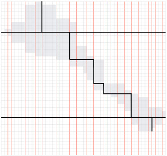
Figure 2: Decomposition of a partial matrix into staircase matrices (defined by solid thick black lines) and into blocks of consecutive columns with the same defined entries (indicated by thin vertical red lines).

It is easy to verify that, in the resulting decomposition, each row is covered by at most two staircase matrices, and each column is covered by at most three staircase matrices. Also note that every set of consecutive columns whose defined elements are in exactly the same set of rows are covered in this decomposition by the same three row-disjoint staircase matrices. ∎

We next prove the fact that, if $M$ is a TM staircase matrix with $m$ rows, then the complexity of its upper envelope is $O(m)$.

Lemma 5

The number of breakpoints in the upper envelope of an $m\times n$ TM staircase matrix is at most $2m$.

Proof

We focus on the case where the defined entries of all rows begin in the first column and end in non-decreasing columns. In other words, for all $i$, $s_{i}$=1 and $t_{i}\leq t_{i+1}$. The other cases are symmetric.

A breakpoint is a situation where the maximum in column $c$ is at row $r_{1}$ and the maximum in column $c+1$ is at a different row $r_{2}$. We say that $r_{1}$ is the departure row of the breakpoint, and $r_{2}$ is the entry row of the breakpoint. There are two types of breakpoints: decreasing ($r_{1}<r_{2}$), and increasing ($r_{1}>r_{2}$). We show that (1) each row can be the entry row of at most one decreasing breakpoint, and (2) each row can be the departure row of at most one increasing breakpoint.

1. Assume that row $r_{2}$ is an entry row of two decreasing breakpoints: One is the pair of entries $(r_{1},c_{1}),(r_{2},c_{1}+1)$ and the other is the pair $(r_{3},c_{2}),(r_{2},c_{2}+1)$. We know that $r_{1}<r_{2}$, $r_{3}<r_{2}$, and wlog $c_{2}>c_{1}+1$. Since the maximum in column $c_{1}+1$ is in row $r_{2}$, we have $M_{r_{3},c_{1}+1}<M_{r_{2},c_{1}+1}$. However, since the maximum in column $c_{2}$ is in row $r_{3}$, we have $M_{r_{3},c_{2}}>M_{r_{2},c_{2}}$, contradicting the total monotonicity of $M$. Note that $M_{r_{2},c_{2}}$ is defined since $M_{r_{2},c_{2}+1}$ is defined.

2. Assume that row $r_{1}$ is a departure row of two increasing breakpoints: One is the pair of entries $(r_{1},c_{1}),(r_{2},c_{1}+1)$ and the other is the pair $(r_{1},c_{2}),(r_{3},c_{2}+1)$. We know that $r_{1}>r_{2}$ and $r_{1}>r_{3}$. Since the maximum in column $c_{1}$ is in row $r_{1}$, we have $M_{r_{2},c_{1}}<M_{r_{1},c_{1}}$. However, since the maximum in column $c_{1}+1$ is in row $r_{2}$, we have $M_{r_{2},c_{1}+1}>M_{r_{1},c_{1}+1}$, contradicting the total monotonicity of $M$. Note that $M_{r_{1},c_{1}+1}$ is defined since $M_{r_{1},c_{2}}$ is defined.

∎

Using Lemmas 4.1 and 5 we can now complete the proof of Theorem 4.1. Let $bp(M_{i})$ denote the number of breakpoints in the upper envelope of $M_{i}$. Let $m_{i}$ denote the number of rows in $M_{i}$. Since each row appears in at most three $M_{i}$s, $\sum_{i}m_{i}=O(m)$. The total number of breakpoints in the envelopes of all of $M_{i}$s is $O(m)$ since $\sum_{i}bp(M_{i})=\sum_{i}O(m_{i})=O(m)$.

Consider now a partition of $M$ into rectangular blocks $B_{j}$ defined by maximal sets of contiguous columns whose defined entries are at the same set of rows. There are $O(m)$ such blocks. The upper envelope of $M$ is just the concatenation of the upper envelopes of all the $B_{j}$’s. Hence, $bp(M)=\sum_{j}bp(B_{j})+O(m)$ (the $O(m)$ term accounts for the possibility of a new breakpoint between every two consecutive blocks). Therefore, it suffices to bound $\sum_{j}bp(B_{j})$.

Consider some block $B_{j}$. As we mentioned above, the columns of $B_{j}$ appear in the same three row-disjoint staircase matrices $M_{1},M_{2},M_{3}$ in the decomposition of $M$. The column maxima of $B_{j}$ are a subset of the column maxima of $M_{1},M_{2},M_{3}$. Assume wlog that the indices of rows covered by $M_{1}$ are smaller than those covered by $M_{2}$, which are smaller than those covered by $M_{3}$.

The breakpoints of the upper envelope of $B_{j}$ are either breakpoints in the envelope of $M_{1},M_{2},M_{3}$, or breakpoints that occur when the maxima in consecutive columns of $B_{j}$ originate in different $M_{i}$. However, since $B_{j}$ is a (non-partial) TM matrix, its column maxima are monotone. So once a column maximum originates in $M_{i}$, no maximum in greater columns will ever originate in $M_{j}$ for $j<i$. It follows that the number of breakpoints in $B_{j}$ that are not breakpoints of $M_{1},M_{2},M_{3}$ is at most two. Since there are $O(m)$ blocks, $\sum_{j}bp(B_{j})\leq\sum_{i}bp(M_{i})+O(m)=O(m)$. This completes the proof of Theorem 4.1.

5 Constant Query-Time Data Structures

In this section we present our data structures that improve the query time to $O(1)$ at the cost of an $n^{\varepsilon}$ factor in the construction time and space for any constant $0<\varepsilon<1$.

We use the following micro data structure that slightly modifies the one of Lemma 1.

Lemma 6 (another micro data structure)

Given a TM matrix of size $x\times n$, one can construct in $O(xn^{\varepsilon}\varepsilon^{-1})$ time and space a data structure that given a query column can report the maximum entry in the entire column in $O(\log(\varepsilon^{-1}))$ time for any $1>\varepsilon\geq\log\log n/\log n$.

Proof

Recall that the data structure of Lemma 1, for $r=1$, finds in $O(x\log n)$ time a set of $O(x)$ values (breakpoints) in the range $\{1,\ldots,n\}$. A query is performed in $O(pred(x,n))$ time using a standard predecessor data structure on these $O(x)$ values. Since now we can allow an $n^{\varepsilon}$ factor we use a non-standard predecessor data structure with faster $O(\varepsilon^{-1})$ query-time. We now describe this data structure.

Consider the complete tree of degree $n^{\varepsilon}$ over the leaves $\{1,\ldots,n\}$. We do not store this entire tree. We only store the leaf nodes corresponding to the $O(x)$ existing values and all ancestors of these leaf nodes. Since the height of the tree is $O(\varepsilon^{-1})$ we store only $O(x\varepsilon^{-1})$ nodes. At each such node we keep two arrays, each of size $n^{\varepsilon}$. The first array stores all children pointers (including null-children). The second array stores for each child $u$ (including null-children) the value $pred(u)=$ the largest existing leaf node that appears before $u$ in a preorder traversal of the tree.

The $y=O(x\varepsilon^{-1})$ nodes are stored in a hash table. We use the static deterministic hash table of Hagerup et al. [18] that is constructed in $O(y\log y)=O(x\varepsilon^{-1}\log(x\varepsilon^{-1}))$ worst case time and can be queried in $O(1)$ worst case time. Upon query, we binary-search (using the hash table) for the deepest node $v$ on the root-to-query path whose child $u$ on the root-to-query path is null. To find the predecessor we use $v$’s second array and return $pred(u)$.

The total construction time is $O(x\log n+xn^{\varepsilon}\varepsilon^{-1}+x\varepsilon^{-1}\log(x\varepsilon^{-1}))$ which is $O(xn^{\varepsilon}\varepsilon^{-1})$ since we assume $\varepsilon\geq\log\log n/\log n$. The query time is $O(\log(\varepsilon^{-1}))$ since we binary-search on a path of length $\varepsilon^{-1}$ and each lookup takes $O(1)$ time using the hash table. ∎

We use the above micro data structure to obtain the following data structure.

Lemma 7

Given a TM $x\times n$ matrix, one can construct in $O(x^{3}n^{\varepsilon}\varepsilon^{-1})$ time a data structure of size $O(x^{3}n^{\varepsilon}\varepsilon^{-1})$ that can report the maximum entry in a query column and a contiguous range of rows in $O(\log(\varepsilon^{-1}))$ time.

Proof

For each of the $O(x^{2})$ row intervals, construct the data structure of Lemma 6. ∎

A constant-query subcolumn data structure.

Lemma 8

Given a TM matrix of size $m\times n$, one can construct, in $O(mn^{\varepsilon}\varepsilon^{-2})=O(n^{1+\varepsilon}\varepsilon^{-2})$ time and space a data structure that can report the maximum entry in a query column and a contiguous range of rows in $O(\varepsilon^{-1}\log(\varepsilon^{-1}))$ time.

Proof

The first idea is to use a degree-$x$ tree, with $x=m^{\varepsilon/4}$, instead of the binary tree $T_{h}$. The height of the tree is $O(\log m/\log x)=O(\varepsilon^{-1})$. The leaves of the tree correspond to individual rows of $M$. For an internal node $u$ of this tree, whose children are $u_{1},u_{2},\dots,u_{x}$ and whose subtree contains $k$ leaves (i.e., $k$ rows), recall that $M^{u}$ is the $k\times n$ matrix defined by these $k$ rows and all columns. Let $\hat{M}^{u}$ be the $x\times n$ matrix whose $(i,j)$ element is the maximum in column $j$ among the rows of $M^{u_{i}}$. In other words, $\hat{M}^{u}(i,j)=\max_{\ell}{M}^{u_{i}}(\ell,j)$.

Working bottom up, for each internal node $u$, instead of explicitly storing the matrix $M^{u}$ (whose size is $O(kn)$), we build the $O(kn^{\varepsilon}\varepsilon^{-1})$-sized micro data structure of Lemma 6 over the $k$ rows of $M^{u}$. This way, any element $\hat{M}^{u}(i,j)$ can be obtained in $O(\log(\varepsilon^{-1}))$ time by querying the data structure of $u_{i}$. Once we can obtain each $\hat{M}^{u}(i,j)$ in $O(\log(\varepsilon^{-1}))$ time, we use this to construct the data structure of Lemma 7 over the $x=m^{\varepsilon/4}$ rows of $\hat{M}^{u}$.

Constructing the micro data structure of Lemma 6 for an internal node with $k$ leaf descendants takes $O(kn^{\varepsilon}\varepsilon^{-1})$ time and space. Summing this over all internal nodes in the tree, the total construction takes $O(mn^{\varepsilon}\varepsilon^{-2})$ time and space. After this, we construct the Lemma 7 data structure for each internal node but we use $\varepsilon/2$ and not $\varepsilon$ so the construction takes $O(x^{3}n^{\varepsilon/2}\varepsilon^{-1}\cdot\log(\varepsilon^{-1}))=O(m^{3\varepsilon/4}n^{\varepsilon/2}\varepsilon^{-1}\log(\varepsilon^{-1}))$ time and space. The total construction time over all $O(m/x)=O(m^{1-\varepsilon/4})$ internal nodes is thus $O(m^{1+\varepsilon/2}n^{\varepsilon/2}\varepsilon^{-1}\log(\varepsilon^{-1}))=O(n^{1+\varepsilon}\varepsilon^{-1}\log(\varepsilon^{-1}))$ time and space.

We now describe how to answer a query. Given a query column and a row interval $I$, there is an induced set of $O(\log m/\log x)=O(\varepsilon^{-1})$ canonical nodes. Each canonical node $u$ is responsible for a subinterval of $I$ (that includes all descendant rows of $u_{i},u_{1+1}\ldots,u_{j}$ for some two children $u_{i},u_{j}$ of $u$). We find the maximum in this subinterval with one query to $u$’s Lemma 7 data structure in $O(\log(\varepsilon^{-1}))$ time. The total query time is thus $O(\varepsilon^{-1}\log(\varepsilon^{-1}))$. ∎

A constant query submatrix data structure.

Theorem 5.1

Given a Monge matrix of size $m\times n$, one can construct, in $O(n^{1+\varepsilon}\varepsilon^{-3}\log(\varepsilon^{-1}))$ time and space, a data structure that can report the maximum entry in a query submatrix in $O(\varepsilon^{-2}\log(\varepsilon^{-1}))$ time.

Proof

As in the proof of Lemma 8, we construct a degree-$x$ tree $T_{h}$ over the rows of $M$, with $x=m^{\varepsilon/4}$. Recall that $T_{h}$ includes, for each internal node $u$, (i) the data structure of Lemma 6, which enables queries to elements of $\hat{M}^{u}$ in $O(\log(\varepsilon^{-1}))$ time, and (ii) the breakpoints of all possible row intervals of the $x\times n$ matrix $\hat{M}^{u}$. In addition to the breakpoints we store, for each of these $O(x^{2})$ intervals, a RMQ data structure over the maximum elements between breakpoints. The construction of those RMQ data structures is described in the sequel.

For each level $\ell>0$ of the $O(\varepsilon^{-1})$ levels of the tree $T_{h}$ (the leaves of $T_{h}$ are considered to be at level 0), we construct the symmetric data structure of Lemma 8 over the $(m/{x^{\ell-1}})\times n$ matrix formed by the union of $\hat{M}^{u}$ over all level-$i$ nodes $u$ in $T_{h}$. We denote these data structures by $\mathcal{B}_{\ell}$. Their construction takes total $O(\varepsilon^{-1}\cdot mn^{\varepsilon}\varepsilon^{-2}\cdot\log(\varepsilon^{-1}))=O(n^{1+\varepsilon}\varepsilon^{-3}\log(\varepsilon^{-1}))$ time and space. For notational convenience we define $B_{0}$ to be equal to $B_{1}$.

We now describe how to construct the RMQ data structures for an internal node $u$ at level $\ell$ of $T_{h}$ with children $u_{1},\dots,u_{x}$. We describe how to construct the RMQ for the interval consisting of all rows of $\hat{M}^{u}$. Handling the other intervals is similar. We need to show how to list the maximum among the column maxima of $\hat{M}^{u}$ between every two consecutive breakpoints of $\hat{M}^{u}$. All the column maxima between any two consecutive breakpoints are contributed by a single known child $u^{\prime}$ of $u$. In other words, we are looking for the maximum element in the range consisting of a single row of $\hat{M}^{u}$ and the range of columns between the two breakpoints. This maximum can be found by querying the $\mathcal{B}_{\ell}$ data structure in $O(\varepsilon^{-1}\log(\varepsilon^{-1}))$ time. There are $O(x)$ such queries for each of the $O(x^{2})$ intervals at each of the $O(m/x)$ internal nodes. Therefore, the total construction time of the RMQs is $O(m^{1+\varepsilon}\cdot\varepsilon^{-1}\log(\varepsilon^{-1}))$. This completes the description of our data structure.

We finally discuss how to answer a query (a range in $M$ of rows $R$ and columns $C$). A query induces a set of $O(\varepsilon^{-1})$ canonical nodes $u$. For a canonical node $u\in T_{h}$ and an induced row interval $R_{u}$, we use the list of breakpoints of $R_{u}$ in $\hat{M}^{u}$ to identify the breakpoints that are fully contained in $C$. This takes $O(\log(\varepsilon^{-1}))$ time. The maximum element in those columns is found by querying the RMQ data structure of $R_{u}$ in $u$. In addition to that, there are at most two column intervals $C^{\prime}$ and $C^{\prime\prime}$ in $\hat{M}^{u}$ that intersect $C$ but are not fully contained in $C$. The maximum in $C^{\prime}\cap C$ and $C^{\prime\prime}\cap C$ is contributed by two known children $u^{\prime},u^{\prime\prime}$ of $u$, respectively. In other words, each of them is the maximum element in the range consisting of a single row of $\hat{M}^{u}$ and a range of columns. If $u$ is a level-$\ell$ node of the tree then we find them by two queries to $\mathcal{B}_{\ell}$: one for the row of $u^{\prime}$ and columns $C^{\prime}$ and one for the row of $u^{\prime\prime}$ and columns $C^{\prime\prime}$. The total query time is thus $O(\varepsilon^{-1}\cdot\varepsilon^{-1}\log(\varepsilon^{-1}))=O(\varepsilon^{-2}\log(\varepsilon^{-1}))$. ∎

References

- [1] A. Aggarwal and M. Klawe. Applications of generalized matrix searching to geometric algorithms. Discrete Appl. Math., 27:3–23, 1990.
- [2] A. Aggarwal, M. M. Klawe, S. Moran, P. Shor, and R. Wilber. Geometric applications of a matrix-searching algorithm. Algorithmica, 2(1):195–208, 1987.
- [3] A. Aggarwal and J. Park. Notes on searching in multidimensional monotone arrays. In 29th FOCS, pages 497–512, 1988.
- [4] S. Alstrup, G. S. Brodal, and T. Rauhe. New data structures for orthogonal range searching. In 41st FOCS, pages 198–207, 2000.
- [5] A. Amir, J. Fischer, and M. Lewenstein. Two-dimensional range minimum queries. In 18th CPM, pages 286–294, 2007.
- [6] G. Borradaile, P. N. Klein, S. Mozes, Y. Nussbaum, and C. Wulff-Nilsen. Multiple-source multiple-sink maximum flow in directed planar graphs in near-linear time. In 52nd FOCS, pages 170–179, 2011.
- [7] G. S. Brodal, P. Davoodi, M. Lewenstein, R. Raman, and S. S. Rao. Two dimensional range minimum queries and Fibonacci lattices. In 20th ESA, pages 217–228, 2012.
- [8] G. S. Brodal, P. Davoodi, and S. S. Rao. On space efficient two dimensional range minimum data structures. In 18th ESA, pages 171–182, 2010.
- [9] R. E. Burkard, B. Klinz, and R. Rudolf. Perspectives of Monge properties in optimization. Discrete Appl. Math., 70:95–161, 1996.
- [10] T. M. Chan, K. G. Larsen, and M. Pǎtraşcu. Orthogonal range searching on the RAM, revisited. In 27th SOCG, pages 354–363, 2011.
- [11] B. Chazelle. A functional approach to data structures and its use in multidimensional searching. SIAM Journal on Computing, 17:427–462, 1988.
- [12] B. Chazelle and L. J. Guibas. Fractional cascading: I. A data structuring technique. Algorithmica, 1:133–162, 1986.
- [13] B. Chazelle and B. Rosenberg. Computing partial sums in multidimensional arrays. In 5th SOCG, pages 131–139, 1989.
- [14] E. D. Demaine, G. M. Landau, and O. Weimann. On Cartesian trees and range minimum queries. Algorithmica, 68(3):610–625, 2014.
- [15] A. Farzan, J. I. Munro, and R. Raman. Succinct indices for range queries with applications to orthogonal range maxima. In 39th ICALP, pages 327–338, 2012.
- [16] M.L. Fredman and D.E. Willard. Trans-dichotomous algorithms for minimum spanning trees and shortest paths. J. Comput. Syst. Sci., 48(3):533–551, 1994.
- [17] H. Gabow, J. L. Bentley, and R.E Tarjan. Scaling and related techniques for geometry problems. In 16th STOC, pages 135–143, 1984.
- [18] T. Hagerup, P. B. Miltersen, and R. Pagh. Deterministic dictionaries. Journal of Algorithms, 41(1):69–85, 2001.
- [19] D. Harel and R. E. Tarjan. Fast algorithms for finding nearest common ancestors. SIAM Journal on Computing, 13(2):338–355, 1984.
- [20] A. J. Hoffman. On simple linear programming problems. In Proc. Symp. Pure Math., volume VII, pages 317–327. Amer. Math. Soc., 1963.
- [21] H. Kaplan, S. Mozes, Y. Nussbaum, and M. Sharir. Submatrix maximum queries in Monge matrices and Monge partial matrices, and their applications. In 23rd SODA, pages 338–355, 2012.
- [22] M. M. Klawe and D. J. Kleitman. An almost linear time algorithm for generalized matrix searching. SIAM Journal Discrete Math., 3:81–97, 1990.
- [23] M. M. Klawe and D J. Kleitman. An almost linear time algorithm for generalized matrix searching. SIAM Journal Discret. Math., 3(1):81–97, 1990.
- [24] G. Monge. Mémoire sur la théorie des déblais et des remblais. In Histoire de l’Académie Royale des Science, pages 666–704. 1781.
- [25] Y. Nekrich. Orthogonal range searching in linear and almost-linear space. Comput. Geom., 42(4):342–351, 2009.
- [26] J. K. Park. A special case of the -vertex traveling-salesman problem that can be solved in time. Inf. Process. Lett., 40(5):247–254, 1991.
- [27] M. Sharir and P. K. Agarwal. Davenport-Schinzel sequences and their geometric applications. Cambridge University Press, New York, USA, 1995.
- [28] A. Tiskin. Fast distance multiplication of unit-Monge matrices. In 21st SODA, pages 1287–1296, 2010.
- [29] H. Yuan and M. J. Atallah. Data structures for range minimum queries in multidimensional arrays. In 21st SODA, pages 150–160, 2010.