Star Polymers Confined in a Nanoslit:
A Simulation Test of Scaling and Self-Consistent Field Theories

Abstract

The free energy cost of confining a star polymer where $f$ flexible polymer chains containing $N$ monomeric units are tethered to a central unit in a slit with two parallel repulsive walls a distance $D$ apart is considered, for good solvent conditions. Also the parallel and perpendicular components of the gyration radius of the star polymer, and the monomer density profile across the slit are obtained. Theoretical descriptions via Flory theory and scaling treatments are outlined, and compared to numerical self-consistent field calculations (applying the Scheutjens-Fleer lattice theory) and to Molecular Dynamics results for a bead-spring model. It is shown that Flory theory and self-consistent field (SCF) theory yield the correct scaling of the parallel linear dimension of the star with $N$, $f$ and $D$, but cannot be used for estimating the free energy cost reliably. We demonstrate that the same problem occurs already for the confinement of chains in cylindrical tubes. We also briefly discuss the problem of a free or grafted star polymer interacting with a single wall, and show that the dependence of confining force on the functionality of the star is different for a star confined in a nanoslit and a star interacting with a single wall, which is due to the absence of a symmetry plane in the latter case.

I Introduction

The physical properties and geometric conformations of macromolecules are strongly affected when these polymers are confined in nanoscopically thin slits or tubes, with linear dimensions in between the size of a monomeric unit and the size of a free macromolecule in solution 1 ; MD_PJdG ; 3 ; 4 ; 5 ; 6 ; 7 ; 8 ; 9 ; 10 ; 11 ; 12 ; 13 ; 14 ; 15 ; 16 ; 17 . For linear macromolecules, this problem has been considered extensively in the literature, but much less attention has been devoted to the related problem of confining polymers with a more complex chemical architecture, such as star polymers with $f$ arms halperin87 ; 19 ; 19' , dendrimers 19 , randomly branched polymers, etc. Such questions are important in various contexts, such as chromatographic separations, colloidal stabilization (recall that a nanocolloid coated with a grafted polymeric brush layer in many respects has properties closely related to a star polymer 20 ), preparation of stimuli-responsive nanomaterials, biomolecules constrained by cell membranes, etc. Understanding such problems first for isolated macromolecules and confining purely repulsive walls is a prerequisite before one can address many related relevant problems such as adsorption of such macromolecules at the confining surfaces 21 ; CNL ; CNL1 , interactions between confined polymers under various conditions 19' ; 22 ; 23 ; Egorov , etc.

In the present work, we examine the generic problem of star polymers under nanoconfinement, focusing on the simple limit where the number of arms $f$ is not excessively large halperin87 ; 24 ; 25 ; 25' , and hence the physical effects of crowding too many arms near the star center need not be considered. As a first step, we formulate in Sec. II a crude version of the Flory theory (where Gaussian entropic elasticity is combined with a mean-field treatment of monomer-monomer-repulsions 26 ). This treatment predicts correctly the dependence of linear dimensions on the number of arms $f$, their chain length $N$, and the width of the slit $D$ (or pore diameter, respectively). However, the corresponding free energies disagree with the pertinent predictions of the scaling theory 24 ; 25 , which is based on the simple blob concepts pioneered by de Gennes and Daoud 1 ; MD_PJdG , or Daoud and Cotton 24 . As is well known, the success of the Flory theory for chain linear dimensions of a single chain is due to the cancellation of errors, although the precise reason for this cancellation is yet unknown 1 .

The free energy of a single chain under good solvent conditions according to Flory theory is predicted to vary like $N^{1/5}$ with chain length $N$ while scaling arguments imply that it is independent of $N$ (of the order of thermal energy $k_{B}T$ 1 ). Thus this partial failure of Flory theory for stars is not unexpected. Furthermore, the Flory treatment cannot describe the smooth crossover to the case of unconfined star when $D$ gets comparable to the diameter of a free star. For the description of this crossover, the lattice formulation fleer93 of the self-consistent field theory (Sec. III) clearly is a more powerful tool, although it shares difficulties with the Flory theory with respect to the scaling properties of the free energy. These problems of self-consistent field theory are also elucidated by presenting results for the simpler problem of confining linear chains in cylindrical tubes, Hsu2 ; Klushin Section III.2. Molecular Dynamics simulations 28 ; 29 ; 30 ; 31 (Sec. IV), on the other hand, can reproduce the scaling predicted by the blob picture. With respect to local effects near the confining walls, we discuss the use of the extrapolation length concept, and find it similarly useful as for confined linear polymers 11 ; 17 . Finally, we also consider the problem of a star polymer interacting with a single wall, and show that the dependence of confining force on the functionality of the star polymer is different for a star confined in a nanoslit and a star interacting with a single wall, which is due to the absence of a symmetry plane in the latter case. Section V then summarizes our conclusions.

II FLORY THEORY OF FREE AND CONFINED STAR POLYMERS

II.1 Unconfined (Free) Stars

The statistical mechanics of star polymers in good solvent has been treated by many elaborate theories, from self-consistent minimization of intramolecular interactions Allegra to renormalization group methods Miyake ; Douglas ; Vlahos ; Duplantier1 ; Duplantier2 ; Ohno . However, to provide a first overview it is nevertheless useful to discuss the simple Flory theory.

According to Flory theory, the free energy of a polymer in the presence of excluded volume interactions is written as a sum of two terms, the first one $({F}_{e\ell})$ corresponds to entropic elasticity of the chain, the second to the (pairwise) interactions between the effective monomers $(F_{\rm int})$, see Grosberg and Khokhlov GK ,

$$F=F_{e\ell}+F_{\rm int}$$ (1)

For a single chain, $F_{e\ell}$ (in units of temperature) is $R^{2}/a^{2}N$, with $a$ the monomer size, $N$ the number of monomers. If $F_{\rm int}$ is negligible, the probability to have a radius $R$ is simply (factors of order unity will be ignored throughout in the following and $k_{B}T\equiv 1$)

$$p(R)\propto\exp(-F_{e\ell}(R))\Rightarrow\langle R^{2}\rangle=a^{2}N,\quad\langle F\rangle=1.$$ (2)

In terms of a blob picture, a free Gaussian chain is a single blob as well. For a free star polymer with $f$ arms linked to a center, we simply have

$$F_{e\ell}(R)=fR^{2}/a^{2}N.$$ (3)

The $f$ Gaussian arms do not disturb each other, each arm has a size $\langle R^{2}\rangle=aN$, and the total free energy then is $\langle F\rangle=f$.

Let us now consider the effect of excluded volume, choosing $V=R^{3}$, $\rho=fN/R^{3}$, to conclude $F_{\rm int}(R)=c\rho^{2}V=c(fN)^{2}/R^{3})$, here $c$ is related to the 2^nd virial coefficient,

$$F=F_{e\ell}(R)+F_{\rm int}(R)=fR^{2}/a^{2}N+c(fN)^{2}/R^{3}.$$ (4)

Minimization gives

$$\partial F/\partial R = 0\Rightarrow 2fR/a^{2}N-3c(fN)^{2}R^{-4}=0,$$

$$R = c^{1/5}a^{2/5}f^{1/5}N^{3/5}.$$ (5)

This equation is in agreement with the Daoud-Cotton result based on the blob picture when one takes for the exponent $\nu$ the Flory value $\nu=3/5$ (see equation (19) of Daoud and Cotton 24 ). In these equations we have assumed for simplicity a constant monomer density inside the volume taken by the star, ignoring the fact that the density near the star core is enhanced. A more elaborate version of Flory theory takes a radial density into account 25' but this does not change the qualitative features of the results.

The free energy then becomes

$$F_{\rm star}\propto c^{2/5}f^{7/5}N^{1/5}.$$ (6)

It is interesting to estimate the free energy from the Daoud-Cotton blob picture which was not done in their paper but has been estimated by Witten and Pincus 25 , who obtained

$$F_{\rm star}\propto f^{3/2}\ln(N).$$ (7)

As discussed by Johner 25' , the mean-field result Eq. (II.1) actually holds for relatively weak excluded volume effects and not so strong stretching of the arms in the star polymer. When the strength of the excluded volume increases, a crossover to a stronger stretching is predicted with a radius of the star polymer scaling as

$$R\propto f^{\frac{1-\nu}{2}}N^{\nu},\quad\nu\approx 0.588$$ (8)

This crossover from Eq. (II.1) to Eq. (8) is missing when one takes the Flory approximation for $\nu$, of course. A similar crossover has also been pointed out for the height of planar brushes, which scales as $h\propto\sigma_{g}^{1/3}N$ in the mean-field regime, yet as $h\propto\sigma_{g}^{\frac{1-\nu}{2\nu}}N$ in the regime where excluded volume is very strong ($\sigma_{g}$ being the grafting density Kreer ; KB ). However, in numerical work it is very difficult to study such small differences between Eqs. (8) and (II.1), or between Eq. (6) and (7) Hsu . Note that Eq. (6) for the single chain ($f=1$) yields the wrong result $F\propto N^{1/5}$, already mentioned in the introduction.

II.2 Confinement of linear chains

When chains are confined by walls, one must take into account that also a Gaussian chain does not penetrate a hard wall and hence there exists a free energy cost of confinement. If a Gaussian chain is confined in a spherical cavity, it experiences a free energy cost of compression (see Eq. 7.2 of the Grosberg-Khokhlov’s book) CNL ; GK .

$$F_{\rm compression}\propto N(a/D)^{2}$$ (9)

One can argue Casassa that the same expression (apart from a prefactor) also holds for confinement in a tube or between plates; note that the result follows from constraining on the accessible positions of chain monomers. Now for Gaussian chains $x,y,z$ components of distance vectors are uncoupled from each other. So the elastic contribution for confinement of Gaussian chains is

$$F_{e\ell}(R)=N(a/D)^{2}+R^{2}/a^{2}N$$ (10)

where the prefactor of the term $N(a/D)^{2}$ [this prefactor is not written!] is $1/3$ of the above prefactor of $F_{\rm compression}$ for planar confinement, and $2/3$ for cylindrical confinement. Here $R$ denotes the chain linear dimension in direction(s) parallel to the confining walls, or along the tube axis, respectively.

For confinement between parallel plates the volumes $V=R^{2}D$ and the density $\rho=N/V=N/(R^{2}D)$, hence

$$F_{\rm conf}=F_{e\ell}(R)+F_{\rm int}(R)=N(a/D)^{2}+R^{2}/a^{2}N+cN^{2}/(R^{2}D)\quad({\rm plates})$$ (11)

From $\partial F_{\rm conf}/\partial R=0$ we find (the first term $N(a/D)^{2}$ does not contribute!)

$$2R/(a^{2}N)-2cN^{2}/R^{3}D=0,\quad R^{4}=ca^{2}N^{3}/D,\quad R=c^{1/4}a^{1/2}D^{-1/4}N^{3/4}$$ (12)

Again, we conclude that the Flory argument provides the correct scaling of $R$ with $D$ and $N$, as suggested by the blob picture GK and stressed already in various previous papers Brochard ; Sung .

For confinement in a tube, the volume is $V=RD^{2}$, the density $\rho=N/V=N/(RD^{2})$ and hence

$$F_{\rm conf}=F_{e\ell}(R)+F_{\rm int}(R)=N(a/D)^{2}+R^{2}/a^{2}N+cN^{2}/(RD^{2})\quad,\quad({\rm tube})$$ (13)

and $\partial F_{\rm conf}/\partial R=0$ then yields

$$2R/(a^{2}N)-cN^{2}/R^{2}D^{2}=0\,\,,\,\,R^{3}=ca^{2}N^{3}/D^{2},\,R=c^{1/3}N(a/D)^{2/3}$$ (14)

Again, the formula for $R$ agrees with the blob picture result GK , but the confinement free energy that Flory theory predicts is incorrect. The blob picture yields (note $g=(D/a)^{1/\nu}$ where $g$ monomers are in a blob of diameter $D$, $F_{\rm conf}=n_{\rm blob}=N/g$)

$$F^{(\rm blob)}_{\rm conf}=N(D/a)^{-1/\nu}=N(D/a)^{-5/3}\quad\quad({\rm plates\;or\;tubes})$$ (15)

in both the plates and tubes cases. This result is not reproduced by Flory theory, which rather yields

$$F^{(\rm Flory)}_{\rm conf}=N(a/D)^{2}+c^{1/2}N^{1/2}(D/a)^{-1/2}\quad\quad({\rm plates})$$ (16)

and

$$F^{(\rm Flory)}_{\rm conf}=N(a/D)^{2}+c^{2/3}N(D/a)^{-4/3}\quad({\rm tubes})$$ (17)

even though the radius $R$ in lateral direction shows the proper scaling. In fact, the competition between the exponents $-2$ and $-1/2$ may lead to an effective exponent. The fact that one cannot rely on Flory prediction for the free energy of confined chains has occasionally been noted before Brochard ; Sung . Note that some authors (e.g., Sung ) did not include the therm $N(a/D)^{2}$ in the elastic part of the free energy, Eq. (10), and thus missed the corresponding term in Eqs. (16), (17).

II.3 Confined Stars

Combining the results of the previous sections, we immediately obtain

$$F_{e\ell}^{\rm conf.star}(R)=fN(a/D)^{2}+fR^{2}/a^{2}N$$ (18)

and, since for confinement in a slit we have $V=R^{2}D$, $\rho=fN/V=fN/R^{2}D$, we obtain $f^{conf.star}_{\rm int}(R)=c(fN)^{2}/R^{2}D$.

Using $F_{\rm conf.star}(R)=F^{conf.star.}_{e\ell}(R)+F^{conf.star}_{\rm int}(R)\quad,\quad\partial F_{conf.star}(R)/\partial R=0$ we get

$$2fR/(a^{2}N)-2c(fN)^{2}/R^{3}D=0,\quad R^{4}=cfN^{3}/D,$$ (19)

and hence

$$R=(cf)^{1/4}(D/a)^{-1/4}N^{3/4}\quad\quad({\rm plates})$$ (20)

This result is in perfect agreement with equation (III-20) of Halperin and Alexander’s paperhalperin87 with respect to the powers of all 4 parameters $c,f,D/a$ and $N$. This result also can be interpreted as the behavior of a two-dimensional star of blobs of diameter $D$, as pointed out by Benhamou et al. 19' .

For confinement in a tube, we would predict ($V=RD^{2}$, $\rho=fN/V=fN/(RD^{2})$)

$$F_{conf.star}(R)=fN(a/D)^{2}+fR^{2}/(a^{2}N)+c(fN)^{2}/(RD^{2})$$ (21)

and hence

$$3F_{conf.star}(R)/\partial R=0\Rightarrow\,\,2Rf/(a^{2}N)-c(fN)^{2}/R^{2}D^{2}=0$$ (22)

and finally $R^{3}=cfN^{3}(a/D)^{2},\quad R=(cf)^{1/3}N(a/D)^{2/3}\quad({\rm tubes})$.

While the blob picture of Halperin and Alexander yields a confinement free energy

$$F^{\rm blob}_{conf.star}\propto fNc^{1/3}(a/D)^{5/3}\quad,$$ (23)

the above treatment gives instead again a competition of terms $D^{-2}$, $D^{-1/2}$.

$$F^{\rm Flory}_{conf.star}\propto fN(a/D)^{2}+c^{1/2}f^{3/2}(D/a)^{-1/2}N^{1/2}\quad({\rm plates})$$ (24)

It is of interest to compare the latter expression to the numerical self-consistent field results which is done in the next section.

III Self-Consistent Field Theory

III.1 Methodology

The central quantity in the self-consistent field (SCF) approach is the mean-field free energy, which is expressed as a functional of the volume fraction profiles and SCF potentials for all components in the system. As explained in detail below, the calculation of the volume fraction profiles and SCF potentials requires solving SCF equations iteratively and numerically, which necessarily involves space discretization, i.e. use of a lattice. In the present work, we employ the method of Scheutjens and Fleerfleer93 which uses the segment diameter $\sigma$ as the size of the cell; throughout this work all the distances are reported in units of the cell size $\sigma$. A three-dimensional version of the SCF theory is formulated on a cubic lattice in Cartesian coordinates.

The star polymer is modeled as a spherical core of radius (not diameter!) $\sigma$ grafted with $f$ chains each of length $N$. In order to model a spherical core on a cubic lattice, we use the previously detailed method,wijmans94 whereby the volume fraction of the core segments, $\phi_{c}(x,y,z)$ is set to unity for the lattice sites located completely inside the core and is set equal to the volume fraction of the (cubic) lattice site located within the sphere for the sites lying on the surface of the core. The grafted polymers are modeled as chains of $N$ monomers all of which are of the same size, with every monomer occupying one lattice site. Grafting is achieved by pinning one end-segment of each of the chains on the spherical core.

In addition to the core and polymer segments (labeled $c$ and $p$, respectively), the system under study also contains (monomeric) solvent and the surface atoms, labeled $v$ and $s$, respectively. The surface atoms are placed in the $x-y$ planes for $z\leq z_{l}$ and $z\geq z_{u}$; their location is “frozen”, i.e. $\phi_{s}(x,y,z)=1$ for the $z$ ranges indicated above and is equal to zero otherwise. The degree of confinement of the star polymer can be varied by changing the width of the planar slit, $D=z_{u}-z_{l}$. Finally, the solvent particles fill all the vacant lattice sites not taken by other species, i.e. SCF calculations are carried out under the incompressibility constraint, meaning that for each lattice site $(x,y,z)$ the sum of the volume fractions of all the species must be equal to unity: $\sum_{i}\phi_{i}(x,y,z)=1$, where $i=c,p,s,$ and $v$.

The SCF approach operates with two key quantities – density distributions of all the species and the corresponding self-consistent field potentials.fleer93 Within our three-dimensional SCF formalism, the density profiles of all the species depend on three Cartesian coordinates, $x,y$, and $z$. In the spirit of a mean-field approach, the potentials represent average interactions of a test molecule with all the other molecules in the system. As such, they depend on the density distributions of the molecules which, in turn, are determined by the potentials. Thus, both quantities must be computed simultaneously and self-consistently via a numerical iterative solution of the SCF equations. In practice, starting from the initial guesses for the volume fraction profiles of all the species, $\phi_{i}(x,y,z)$, one obtains the potentials as follows:fleer93

$$\beta u_{i}(x,y,z)=\beta u^{\prime}(x,y,z)+\sum_{j}\chi_{ij}(<\phi_{j}(x,y,z)>-\phi_{j}^{b}),$$ (25)

where $\phi_{j}^{b}$ is the bulk volume fraction of the component $j$, $\beta=1/k_{B}T$, $k_{B}$ is the Boltzmann constant, and $T$ is the temperature. The first term, which is called the excluded volume potential $u^{\prime}(x,y,z)$, originates from the fact that the SCF equations are solved under the incompressibility constraint specified earlier. The Lagrange multiplier associated with the incompressibility constraint is related to the excluded volume potential $u^{\prime}(x,y,z)$. The second term in Eq. (25) accounts for the energy of the contact interactions between the segments of species $i$ and all other species present in the system, with $\chi_{ij}$ being the corresponding Flory-Huggins interaction parameter. Lastly, the angular brackets in Eq. (25) denote the averaging of the volume fraction profiles over the nearest-neighbor sites according to:

$$<\phi_{i}(x,y,z)>=\frac{1}{6}\sum_{x^{\prime},y^{\prime},z^{\prime}}\phi_{i}(x^{\prime},y^{\prime},z^{\prime})$$ (26)

where $(x^{\prime},y^{\prime},z^{\prime})=(x+\alpha,y+\beta,z+\gamma)$, with $\alpha,\beta,\gamma=-1,1$. We note that for a cubic lattice considered here, the step probabilities to go from one lattice layer to the neighboring one are all equal to 1/6 in $x,y$, and $z$ directions.

Once the SCF potentials are obtained from Eq. (25), one computes the Boltzmann factors associated with these potentials, $G_{i}(x,y,z)=\exp(-\beta u_{i}(x,y,z))$, which enter the calculation of propagators that are necessary to obtain the volume fraction profiles of the polymeric species; the volume fraction profiles for the monomeric species are directly proportional to the corresponding Boltzmann factors.fleer93 The volume fraction profiles thus obtained are compared with the initial guesses substituted into Eq. (25), and the procedure is repeated until self-consistency between input and output profiles is achieved within the desired numerical accuracy.

III.2 Confinement of Single chains: Comparison with Monte Carlo Results

Since the above numerical version of SCF equations deals with polymer chains described by walks on a cubic lattice, where a monomer occupies a lattice site, and neighboring effective monomers along the chain are a lattice spacing apart, the description is reminiscent of the treatment of polymers as self-avoiding walks on the simple cubic lattice. The distinction, of course, is that in the self-avoiding walk (SAW) model the condition that every lattice site can be occupied by a single monomer only, holds strictly while the SCF equations enforce this condition as a statistical average only. Thus, while in the standard SAW model (as studied by extensive Monte Carlo simulation, see e.g. Hsu et al.Hsu2 for work on single chains confined in cylindrical tubes of diameter $D$) the energy cost when two monomers sit on top of each other is infinite, the potential of the SCF equations (Eq. (25)) implies a finite enthalpy cost only. Similarly, in Flory theory the constant $c$ in Eq. (4), (11) - (17) is also related to this finite excluded volume strength.

Nevertheless, it is illuminating to carry out a direct comparison of Monte Carlo data for chains confined in a cylindrical tube with corresponding SCF results (Fig. 1a). Plotting $R_{||}/N^{3/5}$ and $R_{\bot}/N^{3/5}$ vs. $N^{3/5}/D$ one sees a similar quality of scaling, i.e. collapse of the data on master curves, for both approaches. But the SCF results, are shifted to smaller linear dimensions in comparison with the Monte Carlo data, and also the crossover to the “string of blob”-behavior occurs for larger values of $N^{3/5}/D$ only. This discrepancy is easily interpreted: the mean-field description of self-avoidance in terms of Eq. (25) is clearly weaker than the strict SAW condition of the Monte Carlo model. However, it is very plausible, that the SCF equations capture the qualitative features of excluded volume effects correctly, as far as chain linear dimensions are concerned. However, SCF results for the free energy excess due to the confinement perform less well (Fig. 1b). In particular, scaling predicts that $\beta F_{conf}/N\approx const$ and simply varies with $D$ as $D^{-1/\nu}\approx D^{-5/3}$ as long as $D$ is small in comparison to the radius of the free chain, but this is not seen: even for $N$ as large as $N=5000$, the data still depend on $N$ for small $D$. This fact is interpreted by the following consideration: Hsu et al. Hsu2 and Klushin et al. Klushin defined the number of blobs $n_{b}$ as $n_{b}=N(D/a)^{-1/\nu}$, they did not allow for a prefactor (of order unity) in this relation ($a$ is the lattice spacing of the simple cubic lattice). Then they showed that the end-to-end distance $R_{||}$ and the free energy $F$ (in units of $k_{B}T)$ both scale linearly with $n_{b}$ and estimated the prefactors $A$ and $B$ in the relations

$$R_{||}=ADn_{b}\quad,\quad F=Bn_{b}\quad,\quad N\rightarrow\infty$$ (27)

as $A\approx 0.92$, $B\approx 5.33$, for the standard SAW model on the simple cubic lattice.

However, for comparing their results with the present calculation a different definition for the number of blobs (which we denote as $n_{\rm blob}$ in our paper, to distinguish it from the above convention) is more useful. We write

$$n_{\rm blob}=CN(D/a)^{-1/\nu}$$ (28)

where $C$ is a constant that is fixed by the requirement (we always deal with the limit $N\rightarrow\infty$!)

$$R_{||}=Dn_{\rm blob}=CaN(D/a)^{1-1/\nu}\approx CaN(D/a)^{-2/3}\$$ (29)

because the physical picture that the chain is a linear string of $n_{\rm blob}$ blobs of diameter $D$ requires that the prefactor between $R_{||}/D$ and $n_{\rm blob}$ is precisely unity. This consideration immediately yields for the SAW model that $n_{\rm blob}=An_{b}$ and hence $F=B^{\prime}n_{\rm blob}$ with $B^{\prime}\approx 5.79$.

While for the SAW model the above constant $C=1/A\approx 1.09$, for the present SCF calculations it is much smaller, namely $C\approx 0.314$, reflecting the fact that SCF represents a much weaker strength of excluded volume, as noted above (it could be modeled by a Monte Carlo simulation where crossing of chains at the same lattice sites is not strictly forbidden but only requires a finite energy penalty $\varepsilon_{\rm ex}/k_{B}T$). For $D=10$, $N=10^{3}$ we hence find that $n_{\rm blob}\approx 6.8$ and hence we should have $F/N=B^{\prime}n_{\rm blob}/N\approx 0.039$ ($B^{\prime}\approx 5.79$, $n_{\rm blob}\approx 6.8$, $F\approx 39$), which is about a factor of 3 larger than the actual SCF result (see Fig. 1). This consideration shows that SCF cannot be mapped onto the simulation results by rescaling of prefactors.

On the basis of Eq. (17), we expect that SCF theory like Flory theory does not reproduce the blob result $F=B^{\prime}CN(D/a)^{-5/3}$ but rather is described by a competition of two terms, scaling with $D^{-2}$ and $D^{-4/3}$, respectively. But orders of magnitude larger chains would be needed to convincingly demonstrate that.

III.3 SCF results for confined star polymers

From the computed volume fraction profiles, one can readily obtain various structural properties, such as the components of the radius of gyration of the star polymer in the directions parallel ($x$, $y$) and perpendicular ($z$) to the confining plates, e.g.

$$R_{gx}^{2}=\frac{\int_{-\infty}^{\infty}dx\int_{-\infty}^{\infty}dy\int_{z_{l}}^{z_{u}}dz\phi_{p}(x,y,z)x^{2}}{\int_{-\infty}^{\infty}dx\int_{-\infty}^{\infty}dy\int_{z_{l}}^{z_{u}}dz\phi_{p}(x,y,z)},$$ (30)

where $\phi_{p}(x,y,z)$ is the volume fraction of the star polymer segments, while $z_{l}$ and $z_{u}$ are the locations (along the $z$-axis) of the lower and upper confining planes, respectively.

The corresponding numerical SCF results can be compared with the scaling theory. As detailed in the previous Section, the latter predicts the following scaling behavior of the radius of gyration component parallel to confining plates, $R_{g||}$, (i.e. either $R_{gx}$ or $R_{gy}$ for our system): halperin87

$$R_{g||}\sim\sigma f^{1/4}N^{3/4}D^{-1/4},$$ (31)

where good solvent conditions are assumed. Note that exactly the same scaling behavior of $R_{g||}$ is also predicted by the Flory theory.

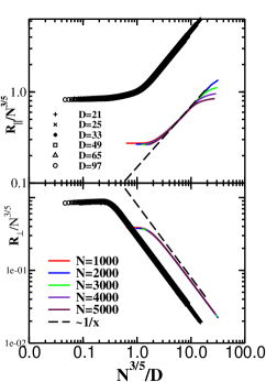
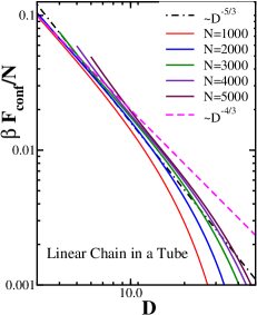
Figure 1: (left) Comparison of MC results (symbols) for the longitudinal and transverse components of a linear chain confined in a tube of diameter $D$ Hsu2 with data from SCF calculations (lines). (right) Variation of the free energy of a linear polymer with tube diameter $D$. Theoretical power laws $~{}D^{-4/3}$ and $D^{-5/3}$ (from Flory theory and blob model, respectively) are included for comparison.

In order to test the above prediction, we have performed SCF calculations for a star polymer for several representative values of $f$ and $N$, the former ranging from $6$ to $12$ and the latter ranging from $250$ to $750$. We gradually varied the degree of confinement by changing the slit width $D$. All the calculations were carried out under good solvent conditions, for non-adsorbing confining walls, i.e. all the Flory-Huggins interaction parameters were set equal to $0$.

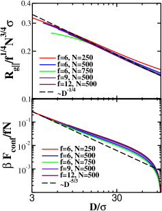
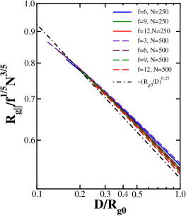
Figure 2: (left) Upper panel: the component of the star polymer radius of gyration parallel to confining plates as a function of the slit width $D$ for several values of $f$ and $N$. Lower panel: the dimensionless confinement free energy of a star polymer (scaled by the product $fN$) as a function of the degree of confinement $D$ for several values of $f$ and $N$. SCF results are shown as solid lines, and scaling predictions are plotted as dashed lines. (right) SCF results for $R_{g||}$ scaled by $R_{g0}$ of unconfined star (i.e., by $f^{1/5}N^{3/5}$) plotted vs scaled degree of confinement $x=D/R_{g0}$. According to scaling predictions, in this form the results in the confined regime for all $f$ and $N$ are expected to collapse onto a single curve $~{}x^{-1/4}$, which is plotted as a dot-dashed line.

The summary of our results for the component of the radius of gyration parallel to confining plates is given in the upper panel of Fig. 2 as a function of the slit width $D$ for several values of $f$ and $N$. One sees that all three scaling predictions given by Eq. (31), i.e. scaling of $R_{g||}^{2}$ with $f^{1/2}$, $N^{3/2}$, and $D^{-1/2}$ are reasonably well confirmed. Alternatively, in the right panel of Fig. 2 we present a different plot where the ratio $R_{g||}/R_{g0}$ of $R_{g||}$ with respect to the unperturbed gyration radius of the star-polymer, $R_{g0}$, is scaled with the dimensionless width of the slit, $x=D/R_{g0}$, where $R_{g0}\propto f^{1/5}N^{3/5}$. According to Eq. (31), one should then observe a decline by power law $\propto\left(D/R_{g0}\right)^{-1/4}$. As can be verified from Fig. 2 (right panel), the SCF results obey the expected scaling reasonably well up to $x\approx 0.3\div 0.4$ and then start deviating from each other and from the $x^{-0.25}$ line.

In addition to the radius of gyration, we have computed free energy of the star polymer confined between two flat plates. As discussed in the previous Section, Flory theory gives the following result for the free energy of confinement:

$$F_{conf.star}=fN(\sigma/D)^{2}+c^{1/2}f^{3/2}(\sigma/D)^{1/2}N^{1/2},$$ (32)

where $c$ is related to second virial coefficient. At the same time, scaling theory predicts: halperin87

$$F_{conf.star}^{scaling}=fNc^{1/3}(\sigma/D)^{5/3}.$$ (33)

In other words, the blob picture predicts a scaling exponent of $-5/3$ for the dependence of the free energy on the slit width, while Flory result is comprised of two terms with two different scaling exponents: $-2$ and $-1/2$.

In the lower panel of Fig. 2 (left), we present the SCF results for the dimensionless confinement free energy, $\beta F_{conf}$, scaled by the product $fN$. The free energy is plotted as a function of the plate separation $D$ for the same pairs of values of $f$ and $N$ as in the upper panel. One sees that while the free energy curves obtained for different values of $f$ and $N$ collapse reasonably well onto a single master curve when scaled by the product $fN$, this curve does not exhibit scaling behavior with $D$ that could be convincingly described by a single scaling exponent (as predicted by Eq. 33), but rather appears to follow the Flory prediction, Eq. (32), which results from the competition of two terms with two different exponents. Unfortunately, the regime where $R_{g||}$ shows the expected power law (for $f=9$ and $f=12,\;f=6$ shows more deviations) as function of $D/\sigma$, Eq. (31), is only about one decade $(6\leq D/\sigma\leq 60)$. In this regime, Eq. (33) clearly is not verified. But one decade is not enough, of course, to prove that there is a competition of two exponents, as found in Eq. (32).

IV Simulation results

IV.1 Molecular Dynamics details

We consider a three-dimensional coarse-grained model grest of a polymer star which consists of $f$ linear arms with one end free and the other one tethered to a microscopic core (seed monomer) of size $R_{c}$ , which is of the order of the monomer size $\sigma$. Each arm is composed of $N$ particles of equal size and mass, connected by bonds. Thus, the total number of monomers in the star (excluding the core) is $fN$. The bonded interactions between subsequent beads is described by the frequently used Kremer-Grest potential kremergrest $V^{\mbox{\tiny KG}}(r)=V^{\mbox{\tiny FENE}}+V^{\mbox{\tiny WCA}}$, with the so-called ’finitely-extensible nonlinear elastic’ (FENE) potential:

$$V^{\mbox{\tiny FENE}}(r)=-0.5kr_{0}^{2}\ln{[1-(r/{r_{0}})^{2}]}$$ (34)

The non-bonded interactions between monomers are taken into account by means of Weeks-Chandler-Andersen (WCA) interaction, i.e., the shifted and truncated repulsive branch of the Lennard-Jones potential given by:

$$V^{\mbox{\tiny WCA}}(r)=4\epsilon\left[(\sigma/r)^{12}-(\sigma/r)^{6}+1/4\right]\theta(2^{1/6}\sigma-r)$$ (35)

In Eqs. (34) and (35), $r$ denotes the distance between the center of two monomers (beads), while the energy scale $\epsilon$ and the length scale $\sigma$ are chosen as the units of energy and length, respectively. Accordingly, the remaining parameters are fixed at the values $k=30\epsilon/\sigma^{2}$, $r_{0}=1.5\sigma$. In Eq. (35) we have introduced the Heaviside step function $\theta(x)=0$ or 1 for $x<0$ or $x\geq 0$. In consequence, the steric interactions in our model correspond to good solvent conditions.

The star-polymer is placed in a slit, i.e., two parallel, repulsive and infinite walls modeled by WCA-potential of Eq. (35) acting only in $z$–direction (perpendicular to the wall). We consider slits widths from $D=3.5\sigma$ up to $D=100\sigma$.

The equilibrium dynamics of the chain is obtained by solving the Langevin equation of motion for the position $\mathbf{r}_{n}=[x_{n},y_{n},z_{n}]$ of each bead in the star,

$$m\ddot{\mathbf{r}}_{n}=\mathbf{F}_{n}^{\mbox{\tiny FENE}}+\mathbf{F}_{n}^{\mbox{\tiny WCA}}-\gamma\dot{\mathbf{r}}_{n}+\mathbf{R}_{n}(t),\qquad(n=1,\ldots,fN)$$ (36)

which describes the Brownian motion of a set of interacting monomers. In Eq. (36) $\mathbf{F}_{n}^{\mbox{\tiny FENE}}$ and $\mathbf{F}_{n}^{\mbox{\tiny WCA}}$ are deterministic forces exerted on monomer $n$ by the remaining bonded and non-bonded monomers, respectively. The influence of solvent is split into slowly evolving viscous force $-\gamma\dot{\mathbf{r}}_{n}$ and rapidly fluctuating stochastic force $\mathbf{R}_{n}$. The random, Gaussian force $\mathbf{R}_{n}$ is related to the friction coefficient $\gamma$ by the fluctuation-dissipation theorem. The integration step was $0.002$ time units (t.u.) and time is measured in units of $\sqrt{m\sigma^{2}/\epsilon}$, where $m$ denotes the mass of the beads, $m=1$. The ratio of the inertial forces over the friction forces in Eq. (36) is characterized by the Reynolds number ${\rm Re}=\sqrt{m\epsilon}/\gamma\sigma$ which in our setup is ${\rm Re}=4$. In the course of our simulation the velocity-Verlet algorithm was employed to integrate the equations of motion (36).

Starting configurations were generated as radially straight chains fixed to the immobile seeded (core) monomer, prior to being placed into a slit with given width $D$. As a next step, star-polymers were equilibrated until they adopted their equilibrium configurations in the confinement geometry. In this step sizes and monomer density profiles have been determined. The required equilibration time depends on $f$ and $N$, ranging from $5\times 10^{5}$ time steps for the smallest stars up to $10^{7}$ for the largest. For star polymers with higher functionality, $f>12$, a larger core bead diameter $\sigma_{core}>\sigma$ has been taken so as to accommodate the $f$-grafting beads of the arms on the surface of the core bead. An initially random placement of these beads on the surface of the core bead has been subsequently rendered to produce a uniform separation between the grafting points (as if being subjected to repulsive Coulomb potential), using the ’diffuse.cpp’ code, developed by J. D. Lettvin Lettvin .

In order to sample the interaction force of a trapped star, for each equilibrated configuration (at a given width $D$), a production run was performed during which time averaged force $\langle\mathcal{F}(t,D)\rangle\equiv\mathcal{F}(D)$ exerted by monomers on both walls as well as monomer density profiles were calculated. The run was continued until uncertainty of the average forces were less than $0.01\sigma$.

IV.2 Numerical results for confined stars

We begin by considering the scaling properties of free unconfined stars, examining the scaling of the mean squared radius of gyration of the star polymers with the number of arms $f$ and their length $N$, the corresponding results are shown in Fig. 3. Since the predicted behavior is $R_{g0}^{2}\propto f^{2/5}N^{2\nu}$, we show a log - log plot of $R_{g0}^{2}f^{-2/5}$ versus $N$, indicating a wide range of $f$-values from $f=3$ to $f=50$. It is clear that this scaling with $f$ cannot be really expected to hold yet for the smallest number of arms, $f=3$, and indeed the data for $f=3$ are slightly off the master curve (which on the log-log plot is the simple straight line corresponding to $R_{g0}^{2}f^{-2/5}=0.4N^{1.18}$).Thus, chain lengths $25\leq N\leq 300$ and number of arms $f\geq 6$ suffice to reach the scaling regime for our simple bead-spring model. We also note here that our scaling results for unconfined stars are in agreement with earlier simulation work of Grest. 28

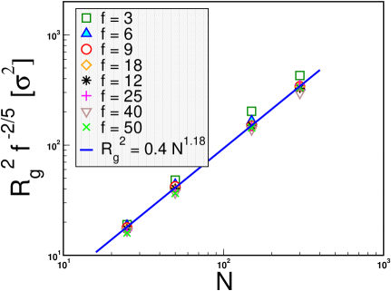
Figure 3: Radius of gyration $R_{g}$ as a function of arm length $N$ and the number of arms $f$ for free star-polymers (no confining walls). MD results are given by symbols, and scaling prediction is indicated by the solid line.

Next, we present the data for the star linear dimensions confined between walls, varying $D$ over a wide range, $3\leq D\leq 60$. Now there is a need to distinguish components $R_{g||}^{2}$ and $R_{g\bot}^{2}$ of the gyration radius parallel and perpendicular to the confining walls. For the free unconfined star (basically reached at $D=60$) we must recover $R_{g\bot}^{2}=R_{g||}^{2}/2$ since then all three Cartesian components $R_{gz}^{2}=R_{g\bot}^{2}$, $R_{gx}^{2}=R_{gy}^{2}=R_{g||}^{2}/2$ are equivalent. Fig. 4 shows that with decreasing $D$ there is a progressing decrease of $R_{g\bot}^{2}$ while $R_{g||}^{2}$ is enhanced. Note also that for a small number of arms ($f=3,6$) there are still rather pronounced statistical inaccuracies which indicate that for confined star polymers with few arms equilibration suffers from unexpectedly large relaxation times. But replotting the data as $R_{g||}^{2}f^{-1/2}$ versus $D$ on a log-log plot, Fig. 4 (inset), shows that we reproduce the predicted behavior $R_{g||}^{2}\propto f^{1/2}D^{-1/2}$.

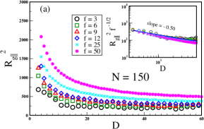
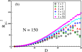
Figure 4: Parallel (a), and perpendicular (b) components of the radius of gyration, $R_{g||}^{2},R_{g\bot}^{2}$, for confined star polymers with different $f$ and $N=150$, plotted as a function of slit width $D$; MD results are given by symbols. In the inset a scaling plot (collapse) of data is displayed in $\log-\log$-coordinates, indicating the predicted relationship $R_{g||}^{2}\propto f^{1/2}\left(\frac{\sigma}{D}\right)^{1/2}N^{3/2}$ (shown by a solid line) halperin87 .

In the Flory theory it was explicitly assumed that inside the disk-like volume taken by the confined star the density of monomers is essentially constant. Fig. 5 indicates that this assumption is a rather poor approximation. Rather the density profile $\rho(z)/\rho(D/2)\propto[(z-\lambda)/D]^{1/\nu}$, if $D$ is large and $z\ll D$. Here an extrapolation length $\lambda=0.51$ is used.

Figure 6 shows the force $\mathcal{F}(D)$ that the monomers of the confined star exert on the walls, choosing slits of widths up to $D=100$. The log-log

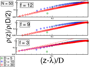
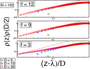
Figure 5: Monomer density profiles for trapped star-polymers presented for $N=50$ [left panel] and $N=150$ [right panel] for various numbers of arms $f$ and slit widths as indicated; MD results are given by symbols. Dashed line (scaling prediction) corresponds to $z^{1/\nu}$, full lines for $f=3$ only: $z^{1.25}$ for $N=50$ and $z\propto z^{1.05}$ for $N=150$.

plot in the inset shows that the data are roughly compatible with the behavior predicted by scaling theory, $\mathcal{F}(D)\propto NfD^{-8/3}$. Since the scaling is not perfect, we have tested for the possible presence of correction terms proportional to $f^{3/2}$ that one might expect when $D$ is of the order of the linear dimension of an unperturbed star, $R_{g0}$. We note that the force of a star interacting with a single wall is predicted to be 30

$$\mathcal{F}(z)\propto f^{3/2}/z,\quad z<R_{g0},$$ (37)

if $z$ is the distance between the star center and the constraining wall; when $D$ is of the order of $R_{g0}$, one might expect that $\mathcal{F}(D)$ is of the same order, i.e. $\mathcal{F}(D)\propto f^{3/2}/D$. To test for this hypothesis, $\mathcal{F}(D)$ for $D=R_{g0}$ is plotted vs $f$ in Fig. 7. One sees, however, that this hypothesis is not fulfilled, the $f$-dependence is much weaker. The reason for this problem is not clear to us.

For the strongly confined stars, on the other hand, the result $\mathcal{F}(D)\propto NfD^{-8/3}$ appears plausible from the snapshot picture, Fig. 8: apart from the region in the immediate neighborhood of the center, the confined star is equivalent to an assembly of $f$ confined linear chains of length $N$, so the system contains $NfD^{-5/3}$ blobs, and this number of blobs is then just the free energy of the confined star.

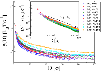
Figure 6: Mean Potential Force $\mathcal{F}(D)$ felt by confined star-polymers vs separation distance $D$ of a slit plotted for different values of $f$ and $N$ as indicated; MD results are given by symbols. The inset displays the same relationship in log-log coordinates; dashed line gives the scaling prediction.

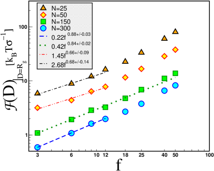
Figure 7: Mean Potential Force $\mathcal{F}(D)$, felt by confined star-polymers vs functionality $f$ in a slit of width $D=R_{g0}$, plotted for different values of $N$ as indicated; MD results are given by symbols, lines are the best fits to MD data.

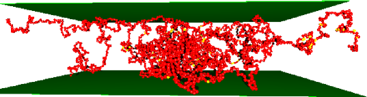
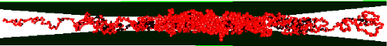
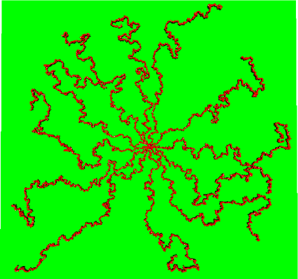
Figure 8: Snapshots of a star polymer with $N=300$ and $f=12$ in a slit with separation between the walls $D=30$ (top), $D=10$ (middle) (side views), and $D=5$ (bottom) (top view).

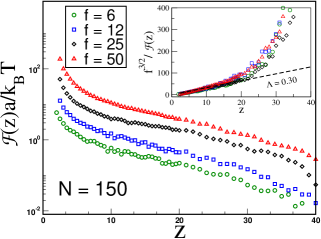
Figure 9: Force exerted on a repulsive wall by a single star polymer with the core monomer fixed at distance $z$ from the wall. Here $N=150$ and the number of arms $f$ is given as parameter; MD results are given by symbols. In the inset one observes a master plot collapse of $\mathcal{F}(z)^{-1}$ for $z\leq 15$, indicating that the force $\mathcal{F}(z)$ and the free energy, $F(z)$, scale $\propto f^{3/2}$ with functionality $f$; dashed line is the scaling prediction.

IV.3 Force between a star polymer and a repulsive wall

As noted above, the force acting from a star polymer interacting with a wall a distance $z$ from its center is predicted to be $\mathcal{F}(z)\propto f^{3/2}/z$, for $z<R_{go}$ (Eq. (37)). However, our results for the force between a star polymer interacting with two walls a distance $D$ apart never gave any evidence for the scaling with $f^{3/2}$. Rather, we found a scaling linear in $f$ for strong confinement (Fig. 6) or even weaker than linear in $f$ for moderate confinement (Fig. 7).

One might suspect that our failure to see a scaling proportional to $f^{3/2}$ could be due to the problem that we are not yet in the regime where a $f^{3/2}$ scaling holds (too short or too few arms, etc.). In order to show that this is not the case, we have studied stars in semi-infinite space, interacting with a wall at distance $z$, for precisely the same choices of $f$ and $N$ as used in the previous section. In practice, in our simulations a “semi-infinite space” also is realized by a film geometry, where one wall is at distance $z$ and the other wall is a distance much larger than $R_{go}$, so that the configuration of the star is not at all affected by this second wall. Fig. 9 gives a plot of our results for $N=150$ and $f$ in the range from $f=6$ to $f=50$. The insert replots these data in the form of $f^{3/2}/f(z)$ versus $z$: one sees that for $3\leq z\leq 50$ the data nicely superimpose on a straight line, in agreement with Eq. (37). Thus, the idea that one can easily relate the problem confining a star with walls at distances $z=D/2$ from both sides, simply has to be abandoned. In the latter case, there are on average always $f/2$ arms in the region above the star center $(D/2<z<D)$ and below it ($0<z<D/2)$. In the case of a single wall, more and more arms move above the star center, the closer the center approaches the wall, and hence the symmetry of the star with respect to the center is completely destroyed. This effect must be responsible for the different scaling behavior with $f$.

V Conclusions

In the paper we have presented a discussion of how confinement of star polymers under good solvent conditions affects their linear dimensions parallel and perpendicular to the confining repulsive parallel walls, and we considered also the free energy cost of confinement (or the related issue of the repulsive force exerted by the macromolecule on these walls). We have restricted attention to the case of long arms of the star polymers (typically we choose $N=150$ in our Molecular Dynamics simulations, but for some purposes both shorter and longer arms, up to $N=300$, have been considered, while for the self-consistent field work somewhat longer chains, from $N=250$ to $N=750$, could be used). The number of arms $f$ was varied from $f=6$ to $f=50$, avoiding the regime where properties are dominated by monomeric crowding near the star center. Although for testing asymptotic scaling relations it would be desirable to be able to study even significantly longer chains, we stress the fact that our work compares well to the regime that would be experimentally accessible (recall that in our coarse-grained model every effective monomer corresponds to a group of about 3 to 5 chemical monomers along the backbone of a real polymer chain molecule.)

We find that both self-consistent field calculations and Molecular Dynamics results confirm a result originally proposed by Halperin and Alexander

halperin87 that radius of the confined star scales with $f,N$ and the distance $D$ between the walls as $R\propto f^{1/4}D^{-1/4}N^{3/4}$, which can be interpreted in terms of the behavior of a two-dimensional star of blobs of diameter $D$. The corresponding confinement free energy $F_{\rm conf}\propto fN(a/D)^{5/3}$, or force on the walls, $\mathcal{F}\propto fN(a/D)^{-8/3}$ is compatible with the MD results, while there seems to be some systematic disagreement with both self-consistent field calculations and the even simpler Flory theory approach. While the latter predicts correctly the scaling of the linear dimensions, this success to some extent is fortuitous, and the free energy is incorrectly predicted, as in the case of the single unconfined chain. We argue that self-consistent field calculations for such confinement problems share some of these problems of Flory theory, despite their much more elaborate character. To elucidate this problem further, we have also performed calculations of linear chains (with $N$ up to $N=5000)$ confined in cylindrical tubes, and compared them to corresponding Monte Carlo calculations. In this context we draw attention to a comparison of self-consistent field calculations and Flory theory with simulations of spherical brushes confined in spherical cavities cerda . They also find that these theories in general fail to reproduce the proper scaling behavior.

While in the general case the theory halperin87 predicts for the confinement free energy a competition of several terms, some of them scaling with $f$ like $f^{3/2}$, and a similar scaling also applies for the force $\mathcal{F}(z)$ between a star polymers at distance $z$ from a wall 30 , $\mathcal{F}(z)\propto f^{3/2}/z$, a relation which we also nicely confirm (Fig. 9), we do not find any evidence for a regime with a $f^{3/2}$ scaling in the confinement free energy (or force $\mathcal{F}(D)$, respectively, see Fig. 7). Presumably, regimes of much larger $N$ and larger $f$ are necessary to elucidate all the different regimes proposed by theory halperin87 .

Acknowledgement: One of us (A.M). thanks the Deutsche Forschungsgemeinschaft (DFG) for support under grant No Bi 314/23, another (S.A.E.) thanks both the DFG (grant No SFB 625/A3) and the Alexander von Humboldt foundation for partial support. We are grateful to H.-P.Hsu for providing us with her data (from Ref. Hsu2 ) for comparison in Fig. 1. Computational time on the PL-Grid Infrastructure is gratefully acknowledged.

References

- (1) P. G. de Gennes, Scaling Concepts in Polymer Physics (Cornell University Press, Ithaca, NY, 1979)
- (2) M. Daoud and P. G. de Gennes, J. Phys. (Paris), 1977, 38, 85.
- (3) K. Kremer and K. Binder, J. Chem. Phys., 1984, 81, 6381.
- (4) A. E. van Giessen and I. Szleifer, J. Chem. Phys., 1995, 102, 9069.
- (5) A. Milchev and K. Binder, J. Phys. II (Paris), 1996, 6, 21.
- (6) K. Binder, A. Milchev and J. Baschnagel, Annu. Rev. Mater. Sci., 1996, 26, 107.
- (7) C. E. Cordeiro, M. Molisana, and D. Thirumalai, J. Phys. II France, 1997, 7, 433.
- (8) E. Eisenriegler, Phys. Rev. E, 1997, 55, 3116.
- (9) A. Milchev and K. Binder, Eur. Phys. J. B, 1998, 3, 477.
- (10) J. de Joannis, J. Jimenez, R. Rajagopalan and I. Bitsanis, Europhys. Lett., 2000, 51, 41.
- (11) A. Milchev and K. Binder, Eur. Phys. J. B, 2000, 13, 607.
- (12) H.-P. Hsu and P. Grassberger, J. Chem. Phys., 2004, 120, 2034.
- (13) G. Morrison and D. Thirumalai, J. Chem. Phys., 2005, 122, 194907.
- (14) T. Sakaue and E. Raphael, Macromolecules, 2006, 39, 2621.
- (15) P. Cifra, J. Chem. Phys., 2009, 131, 224903.
- (16) J. Tang, S. L. Levy, D. W. Trahan, J. L. Jones, H. G. Craighead, and P. S. Doyle, Macromolecules, 2010, 43, 7368.
- (17) A. Milchev, L. I. Klushin, A. M. Skvortsov, and K. Binder, Macromolecules, 2010, 43, 6877.
- (18) A. Halperin and S. Alexander, Macromolecules, 1987, 20, 1146.
- (19) Z. Chen and F. A. Escobedo, Macromolecules, 2001, 34, 6802.
- (20) M. Benhamou, M. Himmi, and F. Benzoine, J. Chem. Phys., 2003, 118, 4759.
- (21) F. Lo Verso, S. A. Egorov, A. Milchev, and K. Binder, J. Chem. Phys., 2010, 135, 184901.
- (22) R. R. Netz and D. Andelman, Phys. Rep., 2003, 380, 1.
- (23) M. Konieczny and C. N. Likos, J. Chem. Phys., 2006, 124, 214904.
- (24) M. Konieczny and C. N. Likos, Soft Matter, 2007, 3, 1130.
- (25) I. Teraoka and P. Cifra, Polymer, 2002, 43, 3025.
- (26) I. Teraoka and Y. Wang, Polymer, 2004, 45, 3835.
- (27) Egorov, S. A.; Paturej, J.; Likos C. N.; Milchev, A., Macromolecules 2013, 46, 3648.
- (28) M. Daoud and J. P. Cotton, J. Phys. (Paris), 1982, 43, 531.
- (29) T. A. Witten and P. A. Pincus, Macromolecules, 1986, 19, 2509.
- (30) A. Johner, Europhys. Lett., 2011, 96, 46004.
- (31) A. Grosberg and A. R. Khokhlov, Statistical Physics of Macromolecules (AIP Press, New York 1994).
- (32) G. J. Fleer, M. A. Cohen-Stuart, J. M. H. J. Scheutjens, T. Cosgrove, and B. Vincent, Polymers at Interfaces (Chapman and Hall, London 1993).
- (33) H.-P. Hsu, K. Binder, L. I. Klushin, and A. M. Skvortsov, Phys. Rev. E, 2008, 78, 041803.
- (34) L. I. Klushin, A. M. Skvortsov, H.-P. Hsu, and K. Binder, Macromolecules, 2008, 41, 5890.
- (35) G. S. Grest, Macromolecules, 1994, 27, 3493.
- (36) A. Jusufi, M. Watzlawek, and H. Löwen, Macromolecules, 1999, 32, 4470.
- (37) A. Jusufi, J. Dzubiella, C. N. Likos, C. von Ferber, and H. Löwen, J. Phys.: Condes. Matter, 2001, 13, 6177.
- (38) S. Huissmann, R. Blaak, and C. N. Likos, Macromolecules, 2009, 42, 2806.
- (39) G. Allegra, E. Colombo, and F. Ganazzoli, Macromolecules, 1993, 26, 330.
- (40) A. Miyake and K. F. Freed, Macromolecules, 1983, 16, 1228.
- (41) J. F. Douglas and K. F. Freed, Macromolecules, 1984, 17, 1854.
- (42) C. H. Vlahos and M. K. Kosmas, Polymer, 1984, 25, 1607.
- (43) B. Duplantier, Phys. Rev. Lett., 1986, 57, 941.
- (44) B. Duplantier and H. Saleur, Phys. Rev. Lett., 1987, 59, 539.
- (45) K. Ohno and K. Binder, J. Chem. Phys., 1991, 95, 5459.
- (46) A. Grosberg and A. R. Khokhlov, in Statistical Physics of Macromolecules, AIP Press 1994, equation 13.2:
- (47) F. Brochard-Wyart and E. Raphael, Macromolecules, 1990, 23, 2276.
- (48) Y. Sung, S. Jun, and B.-Y. Ha, Phys. Rev., 2009, E 79, 061912.
- (49) T. Kreer, S. Metzger, M. Müller, K. Binder, and J. Baschnagel, J. Chem. Phys., 2004, 120, 4012.
- (50) K. Binder, T. Kreer, and A. Milchev, Soft Matter, 2011, 7, 7159.
- (51) H.-P. Hsu, W. Nadler, and P. Grassbereger, Macromolecules, 2004, 37, 4658.
- (52) E.F. Casassa, J. Polym. Sci., 1967, 5, 773.
- (53) C. M. Wijmans, F. A. M. Leermakers, and G. J. Fleer, Langmuir, 1994, 10, 4514.
- (54) G.S. Grest, K. Kremer and T.A. Witten, Macromolecules, 1987, 20, 1376.
- (55) G.S. Grest and K. Kremer, Phys. Rev. A, 1986,33, 3628.
- (56) M. Murat and G.S. Grest, Macromolecules, 1996, 29, 1278.
- (57) J. D. Lettvin (2003): http://lettvin.com/Jonathan/diffuse.cpp
- (58) J. J. Cerda, T. Sintes, and R. Toral, J. Chem. Phys., 2009, 131, 134901.