The blessing of transitivity in sparse and stochastic networks

Abstract.

The interaction between transitivity and sparsity, two common features in empirical networks, implies that there are local regions of large sparse networks that are dense. We call this the blessing of transitivity and it has consequences for both modeling and inference. Extant research suggests that statistical inference for the Stochastic Blockmodel is more difficult when the edges are sparse. However, this conclusion is confounded by the fact that the asymptotic limit in all of the previous studies is not merely sparse, but also non-transitive. To retain transitivity, the blocks cannot grow faster than the expected degree. Thus, in sparse models, the blocks must remain asymptotically small.

Previous algorithmic research demonstrates that small “local” clusters are more amenable to computation, visualization, and interpretation when compared to “global” graph partitions. This paper provides the first statistical results that demonstrate how these small transitive clusters are also more amenable to statistical estimation. Theorem 2 shows that a “local” clustering algorithm can, with high probability, detect a transitive stochastic block of a fixed size (e.g. 30 nodes) embedded in a large graph. The only constraint on the ambient graph is that it is large and sparse–it could be generated at random or by an adversary–suggesting a theoretical explanation for the robust empirical performance of local clustering algorithms.

Introduction

Advances in information technology have generated a barrage of data on highly complex systems with interacting elements. Depending on the substantive area, these interacting elements could be metabolites, people, or computers. Their interactions could be represented in chemical reactions, friendship, or some type of communication. Networks (or graphs) describe these relationships. Therefore, the questions about the relationships in these data are questions regarding the structure of networks. Several of these questions are more naturally phrased as questions of inference; they are questions not just about the realized network, but about the mechanism that generated the network. To study questions in graph inference, it is essential to study algorithms under model parameterizations that reflect the fundamental features of the network of interest.

Sparsity and transitivity are two fundamental and recurring features. In sparse graphs, the number of edges in a network is orders of magnitude smaller than the number of possible edges; the average element has 10s or 100s of relationships, even in networks with millions of other elements. Transitivity describes the fact that friends of friends are likely to be friends. The interaction of these simple and localized features has profound implications for determining the set of realistic statistical models. They imply that in large sparse graphs, there are local and dense regions. This is the blessing of transitivity.

One essential inferential goal is the discovery of communities or clusters of highly connected actors. These form essential feature in a multitude of empirical networks, and identifying these clusters helps answer vital scientific questions in many fields. A terrorist cell is a cluster in the communication network of terrorists; web pages that provide hyperlinks to each other form a community that might host discussions of a similar topic; a cluster in the network of biochemical reactions might contain metabolites with similar functions and activities. Several papers, that are briefly reviewed below, have proved theoretical results for various graph clustering algorithms under the Stochastic Blockmodel, a parametric model, where the model parameters correspond to a true partition of the nodes. Often, these estimators are also studied under the exchangeable random graph model, a non-parametric generalization of the Stochastic Blockmodel. The overarching goal of this paper is to show (1) how sparse and transitive models require a novel asymptotic regime and (2) how the blessing of transitivity makes edges become more informative in the asymptote, allowing for statistical inference even when cluster size and expected degrees do not grow with the number of nodes.

The first part of this paper studies how sparsity and transitivity interact in the Stochastic Blockmodel, and more generally, in the exchangeable random graph model. Interestingly, if a Stochastic Blockmodel is both sparse and transitive, then it has small blocks. The second part of this paper (1) introduces an intuitive and fast local clustering technique to find small clusters; (2) proposes the local Stochastic Blockmodel, which presumes a single stochastic block is embedded in a sparse and potentially adversarially chosen network; and (3) proves that if the proposed local clustering technique is initialized with any point in the stochastic block, then it returns the block with high probability. Figure 1 illustrates the types of clusters found by the proposed algorithm; in this case from a social network on epinions.com containing over 76,000 people.

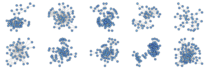
Figure 1. Local clusters from a sparse 76k node social network from epinions.com. Created with the igraph library in R (Csardi and Nepusz, 2006).

0.1. Preliminaries

Networks, or graphs, are represented by a vertex set and an edge set, $G=(V,E)$, where $V=\{1,\dots,n\}$ contains the actors and

$$E=\{(i,j):\mbox{ there is an edge from $i$ to $j$}\}.$$

The edge set can be represented by the adjacency matrix $A\in\{0,1\}^{n\times n}$:

(1) $$A_{ij}=\left\{\begin{array}[]{cl}1&\textrm{ if $(i,j)\in E$}\\ 0&\textrm{ otherwise.}\end{array}\right.$$

This paper only considers undirected graphs. That is, $(i,j)\in E\Rightarrow(j,i)\in E$. The adjacency matrix of such a graph is symmetric. Many of the results in the paper have a simple extension to weighted graphs, where $A_{ij}\geq 0$. For simplicity, we only discuss unweighted graphs. For $i\in V$, let $d_{i}=\sum_{\ell}A_{i\ell}$ denote the degree of node $i$. Define $N_{i}$ as the neighborhood of node $i$,

$$N_{i}=\{j:(i,j)\in E\}.$$

Define the transitivity ratio of $A$ as

$$trans(A)=\frac{\mbox{number of closed triplets in $A$}}{\mbox{number of connected triples of vertices in $A$}}.$$

Watts and Strogatz (1998) introduced an alternative measure of transitivity, the clustering coefficient. The local clustering coefficient, $C(i)$, is defined as the density of the subgraph induced by $N_{i}$, that is the number of edges between nodes in $N_{i}$ divided by the total number of possible edges. The clustering coefficient for the entire network is the average of these values.

$$C=\frac{1}{n}\sum_{i}C(i)$$

This is related to the triangles in the graph because an edge $(j,k)$ between two nodes in $N_{i}$ makes a triangle with node $i$.

0.2. Statistical models for random networks

Suppose $A=\{A_{ij}:i,j\geq 1\}$ is an infinite array that is binary, symmetric, and random. If $A$ is (jointly) exchangeable, that is

$$A\stackrel{{\scriptstyle d}}{{=}}A_{\sigma,\sigma}=\{A_{\sigma(i),\sigma(j)}:i,j\geq 1\},$$

for any arbitrary permutation $\sigma$, then the Aldous-Hoover representation says there exists $i.i.d.$ random variables $\xi_{1},\xi_{2},\dots$ and an additional independent random variable $\alpha$ such that conditional on these variables, the elements of $A$ are statistically independent (Hoover, 1979; Aldous, 1981; Kallenberg, 2005). The global parameter $\alpha$ controls the edge density and for ease of notation, it is often dropped (Bickel et al., 2011). One should think of this result as an extension of DeFinetti’s Theorem to infinite exchangeable arrays.

While this representation has only been proven to be equivalent to exchangeability for infinite arrays, it is convenient to adopt this representation for finite graphs.

Definition 1.

Symmetric adjacency matrix $A\in\{0,1\}^{n\times n}$ follows the exchangeable random graph model if there exists i.i.d. random variables $\xi_{1},\dots,\xi_{n}$ such that probability distribution of $A$ satisfies

$$P(A|\xi_{1},\dots,\xi_{n})=\prod_{i<j}P(A_{ij}|\xi_{i},\xi_{j}).$$

For brevity, we will sometimes refer to this as the exchangeable model.

Independently of the research on infinite exchangeable arrays, Hoff et al. (2002) proposed the latent space model which assumes that (1) each person has a set of latent characteristics (e.g. past schools, current employer, hobbies, etc.) and (2) it is only these characteristics that produce the dependencies between edges. Specifically, conditional on the latent space characteristics, the relationships (or lack thereof) are independent. The Latent Space Model is equivalent to the exchangeable model in Definition 1.

The Stochastic Blockmodel is an exchangeable model that was first defined in Holland and Leinhardt (1983).

Definition 2.

The Stochastic Blockmodel is an exchangeable random graph model with $\xi_{1},\dots,\xi_{n}\in\{1,\dots,K\}$ and

$$P(A_{ij}=1|\xi_{i},\xi_{j})=\Theta_{\xi_{i},\xi_{j}}$$

for some $\Theta\in[0,1]^{K\times K}$.

In this model, the $\xi_{i}$ correspond to group labels. The diagonal elements of $\Theta$ correspond to the probability of within-block connections. The off-diagonal elements correspond to the probabilities of between-block connections. When the diagonal elements are sufficiently larger than the off-diagonal elements, then the sampled network will have clusters that correspond to the blocks in the model.

The next subsection briefly reviews the existing literature that examines the consistency of various estimators for the partition created by the latent variables $\xi_{1},\dots,\xi_{n}$ in the Stochastic Blockmodel.

0.3. Previous research

This paper builds on an extensive body of literature examining various types of statistical estimators for the latent partition $\xi_{1},\dots,\xi_{n}$ in the Stochastic Blockmodel. These estimators fall into four different categories.

1. Several have studied estimators that are solutions to discrete optimization problems (e.g. Bickel and Chen (2009); Choi et al. (2012); Zhao et al. (2011, 2012); Flynn and Perry (2012)). These objective functions are the likelihood function for the Stochastic Blockmodel or the Newman-Girvan modularity (Newman and Girvan, 2004), a measure that corresponds to cluster quality.

2. Others have have studied various approximations to the likelihood that lead to more computationally tractable estimators. For example, Celisse et al. (2011) and Bickel et al. (2012) studied the variational approximation to the likelihood function and Chen et al. (2012a) studied the maximum pseudo-likelihood estimator.

3. Building on on spectral graph theoretic results (Donath and Hoffman, 1973; Fiedler, 1973), several researchers have studied the statistical performance of spectral algorithms for estimating the partition in the Stochastic Blockmodel (McSherry, 2001; Dasgupta et al., 2004; Giesen and Mitsche, 2005; Coja-Oghlan and Lanka, 2009; Rohe et al., 2011; Rohe and Yu, 2012; Chaudhuri et al., 2012; Jin, 2012; Sussman et al., 2012; Fishkind et al., 2013). Others have studied estimators that are solutions to semi-definite programs (Ames and Vavasis, 2010; Oymak and Hassibi, 2011; Chen et al., 2012b).

4. More recently, Bickel et al. (2011); Channarond et al. (2011); Rohe and Yu (2012) have developed methods to stitch together network motifs, or simple “local” measurements on the network, in a way that estimates the partition in the Stochastic Blockmodel. Bickel et al. (2011) draws a parallel between this motif-type of estimator and method of moments estimation.

All of the previous results described above are sensitive to both (a) the population of the smallest block and (b) the expected number of edges in the graph; larger blocks and higher expected degrees lead to stronger conclusions. This limitation arrises because the proofs rely on some form of concentration of measure for a function of sufficiently many variables. Bigger blocks and more edges yield more variables, and thus, more concentration. This paper shows how transitivity leads to a different type of concentration of measure, where each edge becomes asymptotically more informative. As such, the results in this paper extend to blocks of fixed sizes and bounded expected degrees.

Section 2 proposes the LocalTrans algorithm that exploits the triangles built by network transitivity. As such, it is most similar to motif-type estimators in bullet (4). Our analysis of LocalTrans is the first to study whether a local algorithm (i.e. initialized from a single node) can estimate a block in the Stochastic Blockmodel. The emphasis on local structure aligns with the aims of network scan statistics; these compute a “local” statistic on the subgraph induced by $N_{i}$ for all $i$ and then return the maximum over all $i$. In the literature on network scan statistics, Rukhin and Priebe (2012) and Wang et al. (2013) have previously studied the anomaly detection properties under random graph models, including a version of the Stochastic Blockmodel.

1. Transitivity in sparse exchangeable random graph models

In this section, Proposition 1 and Theorem 1 show that previous parameterizations of the sparse exchangeable models and sparse Stochastic Blockmodels lack transitivity in the asymptote. That is, the sampled networks are asymptotically sparse, but they are not asymptotically transitive. Theorem 2 concludes the section by describing a parameterizations that produce sparse and transitive networks.

Define

(2) $$p_{\max}=\max_{\xi_{i},\xi_{j}}P(A_{ij}=1|\xi_{i},\xi_{j})$$

as the largest possible probability of an edge under the exchangeable model. In the statistics literature, previous parameterizations of sparse Stochastic Blockmodels, and sparse exchangeable models, have all ensured sparsity by sending $p_{\max}\rightarrow 0$.

Define

(3) $$p_{\Delta}=P(A_{uv}=1|A_{iu}=A_{iv}=1)$$

a population measure of the transitivity in the model. It is the probability of completing a triangle, conditionally on already having two edges.

By sending $p_{\max}$ to zero, a model removes transitivity.

Proposition 1.

Under the exchangeable random graph model (1)

$$p_{\Delta}\leq p_{\max},$$

where these probabilities are defined in equations (2) and (3).

The next theorem gives conditions that imply the transitivity ratio of the sampled network converges to zero.

Theorem 1.

Under the exchangeable random graph model (Definition 1), define $\lambda_{n}=E(d_{i})$ as the expected node degree. If $\lambda_{n}\rightarrow\infty$, $\lambda_{n}=o(n)$, and

(4) $$p_{\max}=o\left(\frac{P(A_{ij}=1)}{P(A_{ij}=1|A_{i\ell}=1)}\right),$$

where $p_{\max}$ is defined in (2), then $trans(A)\stackrel{{\scriptstyle P}}{{\rightarrow}}0$.

A proof of this theorem can be found in the appendix.

The denominator on the right hand side of Equation (4) quantifies how many edges are adjacent to the average edge, and thus controls how many 2-stars are in the graph. It can be crudely bounded with the maximum expected degree over the latent $\xi_{i}$. For

$$\lambda_{n}^{\max}=\max_{\xi_{i}}\ E(d_{i}|\xi_{i}),$$

it follows that

$$P(A_{ij}=1|A_{i\ell}=1)\leq\lambda_{n}^{\max}/n.$$

Corollary 1.

Under the exchangeable random graph model (Definition 1), define $\lambda_{n}=E(d_{i})$ as the expected node degree. If $\lambda_{n}\rightarrow\infty$, $\lambda_{n}=o(n)$, and

$$p_{\max}=o\left(\frac{\lambda_{n}}{\lambda_{n}^{\max}}\right),$$

then $trans(A)\stackrel{{\scriptstyle P}}{{\rightarrow}}0$.

So, ensuring sparsity by sending $p_{\max}$ to zero removes transitivity both from the model and from the sampled network. The next subsection investigates the implications of restricting $p_{\max}>\epsilon>0$ in sparse networks.

1.1. Implications of non-vanishing $p_{\max}$ in the Stochastic Blockmodel

It is easiest to consider a simplified parameterization of the Stochastic Blockmodel. The following parameterization is also called the planted partition model.

Definition 3.

The four parameter Stochastic Blockmodel is a Stochastic Blockmodel with $K$ blocks, exactly $s$ nodes in each block, $\Theta_{ii}=p$, and $\Theta_{ij}=r$ for $i\neq j$.

In this model, (1) $n=Ks$, (2) the “in-block” probabilities are equal to $p$, and (3) the “out-of-block” probabilities equal to $r$. Moreover, the expected degree of each node is

(5) $$\mbox{Expected degree under the four parameter model}=sp+(n-s)r.$$

Define this quantity as $\lambda_{n}$. Under the four parameter model, $p$ is analogous to $p_{\max}$.

Note that $sp\leq\lambda_{n}$ and

$$n\frac{p}{\lambda_{n}}\leq K.$$

In sparse and transitive graphs, $\lambda_{n}$ is bounded and $p$ is non-vanishing. In this regime, $K$ grows proportionally to $n$. The following proposition states this fact in terms of $s$, the population of each block.

Proposition 2.

Under the four parameter Stochastic Blockmodel, if $p$ is bounded from below, then

$$s=O(\lambda_{n})$$

where $s$ is the population of each block and $\lambda_{n}$ is the expected node degree.

The following Theorem shows that graphs sampled from this parameterization are asymptotically transitive.

Theorem 2.

Suppose that $A$ is the adjacency matrix sampled from the four parameter Stochastic Blockmodel (Definition 3) with $n$ nodes. If $p>\epsilon>0,\ r=O(n^{-1}),$ and $s\geq 3$, then as $n\rightarrow\infty$

$$trans(A)\stackrel{{\scriptstyle P}}{{\rightarrow}}c>0,$$

where $c$ is a constant which depends on $p,r,s$.

Remark: If $r=\frac{c_{0}}{n}$, for some constant $c_{0}$, then

$$c\approx\frac{p^{3}s^{2}}{p^{2}s^{2}+c_{0}^{2}+2spc_{0}}.$$

The appendix contains the proof for Theorem 2.

The fixed block size asymptotics in Theorem 2 align with two pieces of previous empirical research suggesting the “best” clusters in massive networks are small. Leskovec et al. (2009) found that in a large corpus of empirical networks, the tightest clusters (as judged by several popular clustering criteria) were no larger than 100 nodes, even though some of the networks had several million nodes. This result is consistent with findings in Physical Anthropology. Dunbar (1992) took various measurements of brain size in 38 different primates and found that the size of the neocortex divided by the size of the rest of the brain had a log-linear relationship with the size of the primate s natural communities. In humans, the neocortex is roughly four times larger than the rest of the brain. Extrapolating the log-linear relationship estimated from the 38 other primates, Dunbar (1992) suggests that the average human does not have the social intellect to maintain a stable community larger than roughly 150 people (colloquially referred to as Dunbar s number). Leskovec et al. (2009) found a similar result in several other networks that were not composed of humans. The research of Leskovec et al. (2009) and Dunbar (1992) suggests that the block sizes in the Stochastic Blockmodel should not grow asymptotically. Rather, block sizes should remain fixed (or grow very slowly).

1.2. Implications for the exchangeable model

The interaction between sparsity and transitivity also has surprising implications in the more general exchangeable random graph model. To see this, note that in the exchangeable model, it is sufficient to assume that $\xi_{1},\dots,\xi_{n}$ are $i.i.d.$ Uniform$(0,1)$ (Kallenberg, 2005). Then, the conditional density of $\xi_{i}$ and $\xi_{j}$ given $A_{ij}=1$ is

(6) $$c(\xi_{i},\xi_{j})=\frac{P(A_{ij}=1|\xi_{i},\xi_{j})}{P(A_{ij}=1)}$$

When $p_{\max}$ does not converge to zero, there exist values of $\xi_{i}^{*}$ and $\xi_{j}^{*}$ such that $P(A_{ij}=1|\xi_{i},\xi_{j})$ does not converge to zero. However, in a sparse graph, the edge density $P(A_{ij}=1)$ (in the denominator of Equation (6)) converges to zero. So, $c(\xi_{i}^{*},\xi_{j}^{*})$ is asymptotically unbounded. For example, in the popular $P(A_{ij}=1)=O(1/n)$ limit, $c(\xi_{i}^{*},\xi_{j}^{*})$ is proportional to $n$. In a sense, as a sparse and transitive network grows, each edge becomes more informative. This is the blessing of transitivity in sparse and stochastic networks.

This asymptotic setting, where $p_{\max}$ is bounded from below, makes for an entirely different style of asymptotic proof; the asymptotic power comes from the fact that each edge becomes increasingly informative in the asymptote. Previous consistency proofs rely on concentration of measure for functions of several independent random variables (i.e. several edges). In the sparse and transitive asymptotic setting, concentration follows from the blessing of transitivity, allowing asymptotic results with fixed block sizes and bounded degrees. For example, in Theorems 3 and 4 in the next section, neither the block size nor node degree grows in the asymptote.

2. Local ( model + algorithm + results )

This section investigates clustering, or community detection, in sparse and transitive networks. Following the results of the last section, sparse and transitive communities are small. As such, this section is focused on finding small clusters of nodes. In an attempt to strip away as many assumptions as possible from the Stochastic Blockmodel, this section

1. proposes a “localized” model with a small and transitive cluster embedded in a large and sparse graph (that could be chosen by an adversary),

2. introduces a novel local clustering algorithm that explicitly leverages the graphs transitivity, and

3. shows that this local algorithm will discover the cluster in the localized model with high probability.

Similarly to the last section, the interaction between sparsity and transitivity provides for these results, enabling both the fast algorithm and the fixed block asymptotics.

2.1. The local Stochastic Blockmodel

The “local” Stochastic Blockmodel (defined below) presumes that a small set of nodes $S_{*}$ constitute a single block and the model parameterizes how these nodes relate to each other and how they relate to the rest of the network.

Definition 4.

Suppose $A\in\{0,1\}^{(n+s)\times(n+s)}$ is an adjacency matrix on $n+s$ nodes. If there is a set of nodes $S_{*}$ with $|S_{*}|=s$ and

1. $i,j\in S_{*}$ implies $P(A_{ij}=1)\geq p_{in}$,

2. $i\in S_{*}$ and $j\in S_{*}^{c}$ implies $P(A_{ij}=1)\leq p_{out}$,

3. the random variables $\{A_{ij}:\forall i\in S_{*}\mbox{ and }\forall j\}$ are both mutually independent and also independent of the rest of the graph

then $A$ follows the local Stochastic Blockmodel with parameters $S_{*},p_{in},p_{out}$.

The only assumption that this definition makes about edges outside of $S_{*}$ (that is, $(i,j)$ with $i,j\not\in S_{*}$) is that they are independent of the edges that connect to at least one node in $S_{*}$. So, the edges outside of $S_{*}$ could be chosen by an adversary, as long as the adversary does not observe the rest of the graph. The theorems below will add an additional assumption that the average degree (within $S_{*}^{c}$) must be not too large (i.e. it must be sparse).

2.2. Local clustering with transitivity

A local algorithm searches around a seed node for a tight community that includes this seed node. Several papers have demonstrated the computational advantages of local algorithms for massive networks (Priebe et al., 2005; Spielman and Teng, 2008). In addition to fast running times and small memory requirements, the local results are often more easily interpretable (Priebe et al., 2005) and yield what appear to be “statistically regularized” results when compared to other, non-local techniques (Leskovec et al., 2009; Clauset, 2005; Liao et al., 2009). Andersen et al. (2006); Andersen and Chung (2007); Andersen and Peres (2009) have studied the running times and given perturbation bounds showing that local algorithms can approximate the graph conductance. With the exception of Rukhin and Priebe (2012) and Wang et al. (2013), the previous literature has not addressed the statistical properties of local graph algorithms under statistical models.

Given an adjacency matrix $A$ and a seed node $i$, this section defines an algorithm that finds a clusters around node $i$. This algorithm has a single tuning parameter $cut$ that balances the size of the cluster with the tightness of the cluster. Smaller values of $cut$ return looser clusters. The algorithm initializes the cluster with the seed node $S=\{i\}$. It then repeats the following step: For every edge between a node in $S$ ($j\in S$) and a node not in $S$ ($\ell\in S^{c}$), add $\ell$ to $S$ if there are at least $cut$ nodes that connect to both $\ell$ and $j$ (this ensures that $(i,j)$ is contained in at least $cut$-many triangles). Stop the algorithm if all edges across the boundary of $S$ are contained in fewer than $cut$-many triangles.

Algorithm 1 LocalTrans($A,i,cut$)

  1. Initialize set $S$ to contain node $i$.

  2. For each edge $(i,\ell)$ on the boundary of $S$ ($i\in S$ and $\ell\notin S$) calculate $T_{i\ell}$:

$$T_{i\ell}=\sum_{k}A_{ik}A_{k\ell}.$$

  3. If there exists any edge(s) $(i,\ell)$ on the boundary of $S$ with $T_{i\ell}\geq cut$, then add the corresponding node(s) $\ell$ to $S$ and return to step 2.

  4. Return $S$.

Consider LocalTrans$(A,j,\tau)$ as a function that returns a set of nodes, then

$$i\in\texttt{LocalTrans}(A,j,cut)\implies j\in\texttt{LocalTrans}(A,i,cut).$$

Moreover, if $cut^{+}>cut$ then,

$$\texttt{LocalTrans}(A,i,cut^{+})\ \subset\ \texttt{LocalTrans}(A,i,cut).$$

This shows that the results of LocalTrans$(A,i,cut)$, for every node $i$ and every parameter $cut$, can be arranged into a dendogram. LocalTrans only finds one branch of the tree. A simple and fast algorithm can find the entire tree.

To compute the entire dendogram, apply single linkage hierarchical clustering to the similarity matrix

(7) $$T=(AA)\cdot A,\mbox{ where $\cdot$ is element-wise multiplication.}$$

The computational bottleneck of this algorithm is computing $T$, which can be computed in $O(|E|^{3/2})$. Techniques using fast matrix multiplication can slightly decrease this exponent (Alon et al., 1997).

When $A$ contains no self loops, $T_{ij}$ equals the number of triangles that contain both nodes $i$ and $j$. We propose single linkage because it is the easiest to analyze and it yields good theoretical results. However, in some simulation, average linkage has performed better than single linkage. One could also state a local algorithm in terms of average linkage.

Algorithm 2 GlobalTrans($A,\tau$)

  1. Compute the similarity matrix $T=[AA]\cdot A$, where $\cdot$ is element-wise multiplication.

  2. Run single linkage hierarchical clustering on similarity matrix $T$, i.e. grow a maximum spanning tree.

  3. Cut the dendogram at level $\tau$, i.e. delete any edges in the spanning tree with weight smaller than $\tau$.

  4. Return the connected components.

Proposition 3.

Viewing LocalTrans as a function that returns a set of nodes and GlobalTrans as functions that returns a set of sets, $\texttt{LocalTrans}(A,i,\tau)\subset\texttt{GlobalTrans}(A,\tau)$. Moreover,

$$\bigcup_{i}\texttt{LocalTrans}(A,i,\tau)=\texttt{GlobalTrans}(A,\tau).$$

Proof.

Nodes $i$ and $j$ are in the same cluster in both LocalTrans$(A,i,\tau)$ and GlobalTrans$(A,\tau)$ if and only if there exists a path from $i$ to $j$ such that every edge in the path is in at least $\tau$ triangles. ∎

2.3. Local Inference

The next theorem shows that LocalTrans estimates the local block in the Local Stochastic Blockmodel with high probability.

Theorem 3.

Under the local Stochastic Blockmodel (Definition 4), if

$$\sum_{i,j\in S_{*}^{c}}A_{ij}\leq n\lambda,$$

then

1. cut = 1: for all $i\in S_{*}$, LocalTrans$(A,i,cut=1)=S_{*}$ with probability greater than

   $$1-\left(\frac{1}{2}s^{2}(1-p_{in}^{2})^{s-2}+O(p_{out}^{2}ns(s+\lambda))\right).$$

2. cut = 2: for all $i\in S_{*}$, LocalTrans$(A,i,cut=2)=S_{*}$ with probability greater than

   $$1-\left(s^{3}(1-p_{in}^{2})^{s-3}+O(p_{out}^{3}ns(s+\lambda)^{2})\right).$$

See the appendix for the proof of this theorem.

For the local Stochastic Blockmodel to create a transitive block with bounded expected degrees, it is necessary for $p_{in}$ to be bounded from below and for $s$ to be bounded from above. Then, $p_{out}=O(1/n)$ is a sufficient condition for bounded expected degrees. However, because of the inequality in bullet (2) of Definition 4, $p_{out}=O(1/n)$ is not a necessary condition for sparsity. As such, the restriction on $p_{out}$ is particularly relevant. It is also fundamental to the bound in Theorem 3.

The approximation terms $O(p_{out}^{2}ns(s+\lambda))$ and $O(p_{out}^{3}ns(s+\lambda)^{2})$ bound the probability of a connection in $T$ across the boundary of $S_{*}$. The strength of these terms come from the fact that a connection across the boundary requires $cut+1$ simultaneous edges across the boundary of $S_{*}$. Figure 2 gives a graphical explanation for the “+1”. As such, $p_{out}$ is raised to the cut +1 power. When $s$ and $\lambda$ are fixed, then $p_{out}=o(n^{-1/2})$ and $p_{out}=o(n^{-1/3})$ make the approximation term asymptotically negligible for the case $cut=1$ and $cut=2$, respectively. Both of these settings allow the nodes in $S_{*}$ have (potentially) large degrees. If $p_{out}=O(n^{-1})$, then the approximation terms become $O(n^{-1})$ and $O(n^{-2})$ respectively.

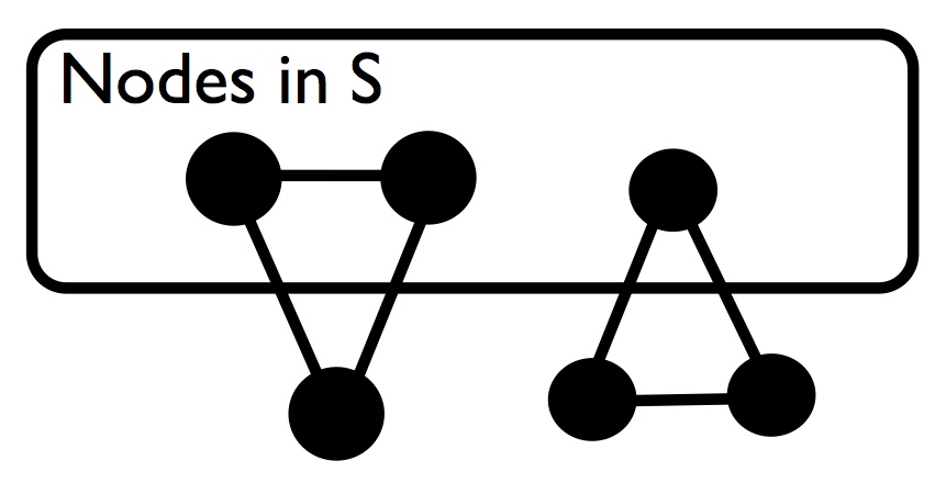
Figure 2. This figure illustrates the two types of triangles that contain nodes in both $S_{*}$ and $S_{*}^{c}$. To make one triangle that crosses the boundary of $S$ requires two edges to cross the boundary.

Theorem 2 and the algorithms LocalTrans and GlobalTrans all leverage the interaction between transitivity and sparsity, making the task of computing $S$ and estimating $S_{*}$ both algorithmically tractable and statistically feasible.

2.4. Preliminary Data Analysis

This section applies GlobalTrans to an online social network from the website slashdot.org, demonstrating the shortcomings of the proposed algorithms with input $A$ and motivating the next section that uses the graph Laplacian as the input. The slashdot network contains 77 360 nodes with an average degree of roughly 12 (Leskovec et al., 2009). This network is particularly interesting because it has a smaller transitivity ratio $(.024)$ than the typical social network.

Figure 3. This plots the number of nodes in the largest ten clusters (ignoring a single giant cluster) found by GlobalTrans$(A,cut)$ in the slashdot social network. These clusters are very small, and probably too small for many applications. Moreover, there are not that many of them.

Figure 3 plots the size of the ten largest clusters returned by GlobalTrans$(A,cut)$ as a function of $cut$ (excluding the largest cluster that consists of the majority of the graph). The values of $cut$ range from 3 to 500 and they are plotted on the $\log_{e}$ scale. Over this range of $cut$, only two times does a cluster exceed ten nodes. While we motivated the local techniques as searching for small clusters, these clusters are perhaps too small. It suggests that there are no clusters that are adequately described by the local Stochastic Blockmodel.

One potential reason for this failure is that under the Local Stochastic Blockmodel, the probability of a connection between a node in $S_{*}$ and a node in $S_{*}^{c}$ is uniformly bounded by some value, $p_{out}$. The slashdot social network, like many other empirical networks, has a long tailed degree distribution. A more realistic model might allow the nodes in $S_{*}$ to be more highly connected to the high degree nodes in $S_{*}^{c}$. The next subsection (1) proposes a “degree-corrected” local Stochastic Blockmodel, (2) proves that LocalTrans with a simple adjustment can estimate $S_{*}$ in the degree corrected model, and (3) demonstrates how this new version of the algorithm improves the results on the slashdot social network.

3. The Degree-corrected Local Stochastic Blockmodel

Inspired by Karrer and Newman (2011), the degree-corrected model in Definition 5 makes the probability of a connection between a node $i\in S_{*}$ and a node $j\not\in S_{*}$ scale with the degree of node $j$ on the subgraph induced by $S_{*}^{c}$.

(8) $$d_{j}^{*}=\sum_{\ell\in S_{*}^{c}}A_{\ell j}$$

For the following definition to make sense, we presume that $d_{j}^{*}$ is fixed for all $j\in S_{*}^{c}$.

Definition 5.

Suppose $A\in\{0,1\}^{(n+s)\times(n+s)}$ is an adjacency matrix and $S_{*}$ is a set of nodes with $|S_{*}|=s$. For $j\in S_{*}^{c}$, define $d_{j}^{*}$ as in Equation (8). If

1. $i\in S_{*}$ and $j\in S_{*}^{c}$ implies

   $$P(A_{ij}=1)\leq\frac{d_{j}^{*}}{n},$$

2. $i,j\in S_{*}$ implies $P(A_{ij}=1)\geq p_{in}$,

3. $\{A_{ij}:\forall j\mbox{ and }\forall i\in S_{*}\}$ are mutually independent

then $A$ follows the local degree-corrected Stochastic Blockmodel with parameters $S_{*},p_{in}$.

The fundamental difference between the previous local model and this degree corrected version is the assumption that if $i\in S_{*}$ and $j\in S_{*}^{c}$, then

$$P(A_{ij}=1)\leq\frac{d_{j}^{*}}{n}.$$

In the previous model, $P(A_{ij}=1)\leq p_{out}$. This new condition can be interpreted as $P(A_{ij}=1)\leq p_{out}\hskip 2.8903ptd_{j}^{*}$ for $p_{out}=1/n$. In this degree-corrected model, the nodes in $S_{*}$ connect to more high degree nodes than they do under the previous local model.

The degree corrected model creates two types of problems for LocalTrans$(A,i,\tau)$. Because the high degree nodes in $S_{*}^{c}$ create many connections to the nodes in $S_{*}$, it is more likely to create triangles with two nodes in $S_{*}$. Additionally, by definition, the high degree nodes outside of $S_{*}$ have several neighbors outside of $S_{*}$. As such, it is more likely to create triangles with one node in $S_{*}$ and two nodes outside of $S_{*}$. In essence, the high degree nodes create several triangles in the graph, washing out the clusters that LocalTrans$(A,i,\tau)$ can detect. To confront this difficulty, it is necessary to down weight the triangles that contain high degree nodes.

3.0.1. The graph Laplacian

Similarly to the adjacency matrix, the normalized graph Laplacian represents the graph as a matrix. In both spectral graph theory and in spectral clustering, the graph Laplacian offers several advantages over the adjacency matrix (Chung, 1997; Von Luxburg, 2007). The spectral clustering algorithm uses the eigenvectors of the normalized graph Laplacian, not the adjacency matrix, because the normalized Laplacian is robust to high degree nodes (Von Luxburg, 2007).

For adjacency matrix $A$, define the diagonal matrix $D$ and the normalized graph Laplacian $L$, both elements of $R^{n\times n}$, in the following way

(9) $$\begin{array}[]{rll}D_{ii}&=&d(i)\\ L_{ij}&=&[{D}^{-1/2}A{D}^{-1/2}]_{ij}=\frac{A_{ij}}{\sqrt{D_{ii}D_{jj}}}.\end{array}$$

Some readers may be more familiar defining $L$ as $I-D^{-1/2}WD^{-1/2}$. For our purposes, it is necessary to drop the $I-$.

The last section utilized the matrix $T=[AA]\cdot A$ to find the triangles in the graph. To confront the degree corrected model, the next theorem uses $[LL]\cdot L$ instead. The interpretation of this matrix is similar to $T$. It differs because it down weights the contribution of each triangle by the inverse product of the node degrees. For example, where a triangle between nodes $i,j,k$ would add 1 to element $T_{ij}$, it would add $(d(i)d(j)d(k))^{-1}$ to the $i,j$th element of $[LL]\cdot L$.

Some versions of spectral clustering use the random walk graph Laplacian, an alternative form of the normalized graph Laplacian.

$$L_{RW}=D^{-1}A$$

While the algorithmic results from spectral clustering can be depend on the choice of graph Laplacian, LocalTrans returns exactly the same results with $L$ as it does with $L_{RW}$. To see this, first imagine that if the graph is directed, then $A$ is asymmetric, and for $T$ to correspond to directed cycles of length three, it is necessary to take the transpose of the final $A$, that is $[AA]\cdot A^{T}$. Since $L_{RW}$ is asymmetric, it is reasonable to use the additional transpose from the directed formulation. It is easy to show that

(10) $$[LL]\cdot L=[L_{RW}L_{RW}]\cdot L_{RW}^{T}.$$

Chaudhuri et al. (2012) and Chen et al. (2012a) have recently proposed a “regularized” graph Laplacian. Chaudhuri et al. (2012) propose replacing $D$ with $D_{\tau}=D+\tau I$, where $\tau>0$ is a regularization constant. They show that a spectral algorithm with

$$L_{\tau}=D_{\tau}^{-1/2}AD_{\tau}^{-1/2}\$$

has superior performance on sparse graphs. Similarly, it will help to use $L_{\tau}$ with LocalTrans. (Note that the equivalence in Equation (10) still holds with the regularized versions of the Laplacians.)

The next theorem shows that under the local degree-corrected model — with the regularized graph Laplacian, a specified choice of tuning parameter $cut$, and $i\in S_{*}$ — the estimate LocalTrans$(L_{\tau},i,cut)=S_{*}$ with high probability. Importantly, using $L_{\tau}$ instead of $A$ allows for reasonable results under the degree-corrected model.

Theorem 4.

Let $A$ come from the local degree-corrected Stochastic Blockmodel. Define $\lambda$ such that

(11) $$\sum_{i,j\in S_{*}^{c}}A_{ij}\leq n\lambda.$$

Set $cut=[2(s-1)p_{in}+2\lambda+\tau]^{-3}$. If

$$n\geq 3\left(2(s-1)p_{in}+2\lambda+\tau\right)^{3/\epsilon}\tau^{-1/\epsilon},$$

and $s\geq 3$, then for any $i\in S_{*}$,

$$\texttt{LocalTrans}(L_{\tau},i,cut)=S_{*}$$

with probability at least

$$1-\left(\nicefrac{{1}}{{2}}\ s^{2}(1-p_{in}^{2})^{s-2}+s\exp\left(-\nicefrac{{1}}{{4}}\ sp_{in}+\lambda\right)+O(n^{3\epsilon-1})\right).$$

A proof of Theorem 4 can be found in the Appendix.

Because simple summary statistics (of sparsity and transitivity) on empirical networks contradict the types of models studied in the literature, Theorem 4 tries to minimizes the assumptions on the “global” structure of the graph. It only assumes that the graph outside of $S_{*}$, i.e. the induced subgraph on $S_{*}^{c}$, is sparse. There are no other assumptions on this part of the graph.

This result is asymptotic in $n=|S_{*}^{c}|$, with $S_{*}$ fixed and containing nodes with bounded expected degree; the assumption in Equation 11 and the definition of $d_{j}^{*}$ imply that the nodes in $S_{*}$ have expected degree less than $s+\lambda$.

3.1. Preliminary Data Analysis

Figure 4. A plot of the number of nodes in the largest ten clusters (ignoring one very large cluster) found by GlobalTrans$(L_{\tau},cut)$ in the slashdot social network. GlobalTrans with $L_{\tau}$ instead of $A$ finds much larger clusters.

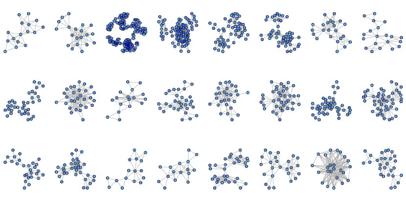
Figure 5. Twenty-four small clusters from the slashdot data set. Because GlobalTrans discovers small clusters, one can easily plot and visualize the clusters with a standard graph visualization tool (Csardi and Nepusz, 2006). The point of this figure is to show the variability in cluster structures; some are tight, clique-like clusters; others are small lattice-like clusters; others are “stringy” collections of three or four tight clusters. This highlights the ease of visualizing the results of local clustering.

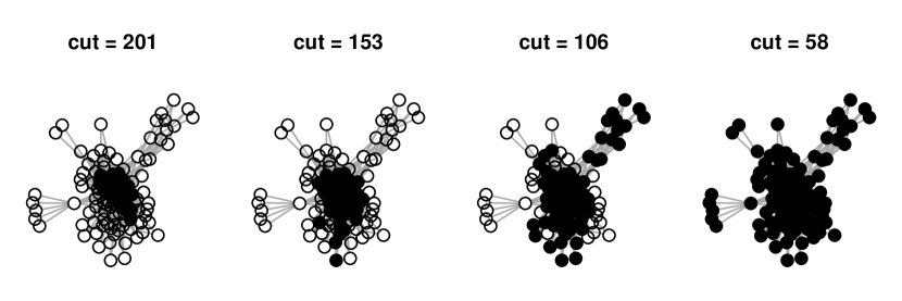
Figure 6. Starting from a seed node, this figure demonstrates how LocalTrans$(L_{\tau=12},i,cut)$ grows as $cut$ decreases. In each panel, the graph is drawn for the smallest value of $cut$, and the solid nodes correspond to the nodes returned by LocalTrans$(L_{\tau=12},i,cut)$, where the value of $cut$ is given above the graph in the units $10^{-6}$. Moving from left to right, the clusters grow larger, and the additional nodes start to extend to the periphery of the visualization.

Recall that Figure 3 illustrates how GlobalTrans$(A,cut)$ fails to find any clusters larger than twenty nodes in the slashdot social network. Figure 4 shows that using $L_{\tau}$ instead of $A$ corrects for the problems observed in Figure 3. It plots the size of the largest ten clusters in the slashdot social network found by GlobalTrans$(L_{12},cut)$ for values of $cut$ between $3*10^{-6}$ and $500*10^{-6}$. It finds several clusters that exceed twenty nodes. In this analysis, and all other analyses using $L_{\tau}$, the regularization constant $\tau$ is set equal to the average node degree (as suggested in Chaudhuri et al. (2012)). In this case, $\tau\approx 12$.

Figure 5 shows some of the clusters from the slashdot social network. Specifically, it plots twenty-four of the induced subgraphs from GlobalTrans$(L_{\tau=12},cut=32*10^{-6})$. Because the clusters are not so large, the sub-graphs are easily visualized and it is easy to see how these clusters have several different structures. Some are nearly planar; others appear as densely connected, “clique-like” sub-graphs; other clusters are a collection of several smaller clusters, weakly strung together. Figure 1 in the introduction gives a similar plot for the epinions social network. These visualizations were created using the graph visualization tool in the igraph package in R (Csardi and Nepusz, 2006).

Figure 6 illustrates how LocalTrans$(L_{\tau=12},i,cut)$ changes as a function of $cut$ for a certain node in the epinions social network. Each of the four panels displays the network for $cut=58*10^{-6}$. In each of the four panels, solid nodes are the nodes that are included in LocalTrans$(L_{\tau=12},i,cut)$ for four different values of $cut$. This seed node was selected because the local cluster is slowly growing as $cut$ decreases and you can see in this in Figure 6. The left most panel displays the results for the largest value of $cut$. This returns the smallest cluster and not surprisingly, the igraph package plots these nodes in the center of the larger graph. Moving to the right, the clusters grow larger and the additional nodes start to extend to the periphery of the visualization. While the clusters for this node grow slowly, for many other nodes, the transitions are abrupt. For example, the nodes that join the cluster in the last panel in Figure 6 jump from cluster sizes of one or two into this bigger cluster. Then, decreasing $cut$ a little bit more, this cluster becomes part of a giant component.

4. Discussion

The tension between transitivity and sparsity in networks that implies that there are local regions of the graph that are dense and transitive. This leads to the blessing of dimensionality, which says that edges (in sparse and transitive graphs) become asymptotically more informative. For example, under the exchangeable model, if the model is sparse and transitive, then the conditional density of the latent variables $\xi_{i},\xi_{j}$, given $A_{ij}=1$, is asymptotically unbounded, concentrating on the values of $\xi_{i},\xi_{j}$ that are consistent with the local structure in the model. This has important implications for statistical models, methods, and estimation theory.

In sparse and non-transitive Stochastic Blockmodels, the block structure is not revealed in the local structure of the network. Rather, the blocks are revealed by comparing the edge density of various partitions. However, under transitive models, the local structure of the network can reveal the block structure. As such, these blocks can be estimated by fast local algorithms. Theorems 3 and 4 show that LocalTrans performs well under a local Stochastic Blockmodel that makes minimal assumptions on the nodes outside of the true cluster; this is the first statistical result to demonstrate how local clustering algorithms can be robust to vast regions of the graph.

This paper studies small clusters because (1) they can create sparse and transitive Stochastic Blockmodels, (2) they are relatively easy to find, both computationally and statistically, and (3) they are easy to plot and visualize. In future research, we will study how these ideas can be used to find large partitions in networks. Sparse and transitive models do not preclude large partitions, as long as some type of local structure exists within each partition. It is not yet clear how global algorithms like spectral clustering might leverage this transitive structure in a stochastic model; this is one area for future research.

Appendix A Proofs for Section 1

A.1. Proof of Theorem 1

Proof.

Recall that the transitivity ratio of $A$ is

$$trans(A)=\frac{\mbox{number of closed triplets in $A$}}{\mbox{number of connected triples of vertices in $A$}}.$$

Both the numerator and the denominator of the transitivity ratio have other formulations that suggest how they can be computed.

number of closed triplets in $$A = 6\times\mbox{Number of triangles in $A$}$$

$$= \mbox{trace}(AAA)$$

number of connected triples of vertices in $$A = 2\times\mbox{Number of 2-stars in $A$}$$

$$= 2\sum_{j}{d_{j}\choose 2}$$

$$= \sum_{j}d_{j}^{2}-d_{j}.$$

For ease of notation, define $X_{n}=trace(AAA)$ and $Y_{n}=\sum_{i}d_{i}^{2}-d_{i}$. So, $trans(A)=X_{n}/Y_{n}$. To show that transitivity converges to zero, use

$$P\left(\frac{X_{n}}{Y_{n}}>\epsilon\right)\leq\frac{E(X_{n}/Y_{n})}{\epsilon}$$

and the following Lemma.

Lemma 1.

If $\lambda_{n}=o(n)$, then there exists a sequence $f_{n}$ such that $E(X_{n})=o(f_{n})$ and

$$P(Y_{n}\geq f_{n})\rightarrow 1.$$

Using Lemma 1 and fact that $X_{n}/Y_{n}\leq 1$ a.s.,

$$E\frac{X_{n}}{Y_{n}} \leq E\left(\frac{X_{n}}{f_{n}}1\{Y_{n}>f_{n}\}+1\{Y_{n}<f_{n}\}\right)$$

$$\leq \frac{E(X_{n})}{f_{n}}+P(Y_{n}<f_{n})$$

$$\rightarrow 0.$$

Now, to prove Lemma 1. For ease of notation, define $d=\sum_{i}d_{i}$. From Bickel, Levina, Chen, define $\hat{\rho}=\frac{d}{2n(n-1)}$. They show that $\hat{\rho}/\rho_{n}\stackrel{{\scriptstyle P}}{{\rightarrow}}1$, where $\rho_{n}=P(A_{12}=1)$. So, this converges to zero:

$$P\left(\frac{d}{2n(n-1)\rho_{n}}<1/2\right)=P\left(d<n(n-1)\rho_{n}\right)$$

Define $M_{n}=n(n-1)\rho_{n}$. Then, $P\left(d>M_{n}\right)\rightarrow 1$. Define $f_{n}=M_{n}^{2}/n-M_{n}$. Notice that

$$min_{\sum_{i}d_{i}=m}\sum_{i}d_{i}^{2}-d_{i}\geq n((m/n)^{2}-m/n)=m^{2}/n-m.$$

Putting these pieces together,

$$P(Y_{n}\geq f_{n}) = \int_{\Omega}1\{Y_{n}\geq f_{n}\}dP$$

$$\geq \int_{d>M_{n}}1\{\sum_{i}d_{i}^{2}-d\geq f_{n}\}dP$$

$$= \sum_{m>M_{n}}\int_{d=m}1\{\sum_{i}d_{i}^{2}-d\geq f_{n}\}dP$$

$$\geq \sum_{m>M_{n}}\int_{d=m}1\{m^{2}/n-m\geq f_{n}\}dP$$

$$= \sum_{m>M_{n}}\int_{d=m}dP$$

$$= P(d>M_{n})\rightarrow 1.$$

The last piece is to show that $E(X_{n})=o(f_{n})$. From the definition of $f_{n}$ and the fact that $\rho_{n}=\lambda_{n}/n$,

$$f_{n} = \frac{\left(n(n-1)\rho_{n}\right)^{2}}{n}-n(n-1)\rho_{n}$$

$$= n(n-1)^{2}(\lambda_{n}/n)^{2}-n(n-1)\lambda_{n}/n$$

$$= \lambda_{n}(n-1)\left(\frac{n-1}{n}\lambda_{n}-1\right)$$

$$\rightarrow \lambda_{n}^{2}n$$

Define

$$S_{12}=\sum_{i}A_{i1}A_{2i}$$

as the number of two stars with nodes 1 and 2 as end points. Then, under the assumption that

$$p_{\max}=o\left(\frac{P(A_{13}=1)}{P(A_{13}=1|A_{23}=1)}\right),$$

it follows that

$$E(X_{n}) = p_{ct}n(n-1)E(S_{12})$$

$$\leq p_{\max}n^{2}(nE(A_{13}A_{23}))$$

$$= p_{\max}n^{3}E(A_{13}|A_{23}=1)E(A_{23}=1)$$

$$= o(\rho_{n}^{2}n^{3})$$

$$= o(f_{n}).$$

∎

A.2. Proof of Theorem 2:

Proof.

Let $r=c_{0}/n$ and let $p$ be fixed.

Number of triangles: Let $\Delta_{n}$ denote the number of triangles. Notice that there are three types of triangles: (1) let $\Delta^{i}$ denote the number of triangles with all nodes in block $i$; (2) let $\Delta_{21}$ denote the number of triangles with 2 nodes in the same block and one node in a separate block; (3) let $\Delta_{111}$ denote the number of triangles with nodes in three separate blocks.

$$E(\Delta_{21})=K(K-1){s\choose 2}spr^{2}=K(K-1){s\choose 2}spc_{0}^{2}/(s^{2}K^{2})\leq p(s-1)/2,$$

$$E(\Delta_{111})={K\choose 3}s^{3}r^{3}\leq K^{3}s^{3}c_{0}^{3}/(6s^{3}K^{3})=c_{0}^{3}/6.$$

By the Markov inequality, $\Delta_{21}/K\stackrel{{\scriptstyle P}}{{\rightarrow}}0,\Delta_{111}/K\stackrel{{\scriptstyle P}}{{\rightarrow}}0$. Finally, $\Delta^{i}$ are iid. So, by LLN, their average converges in probability to their expectation. Putting these pieces together with Slutsky’s theorem, the number of triangles over $K$ is,

$$\frac{1}{K}\Delta_{n}\stackrel{{\scriptstyle P}}{{\rightarrow}}E(\Delta^{i})={s\choose 3}p^{3}.$$

Number of two stars: Let $S_{n}$ be the number of two-stars. Define the events $B=\{|S_{n}-E(S_{n})|>t\}$ and $A=\{\mbox{Maximum Degree}\leq M\}$

$$P(B)=P(BA)+P(BA^{c})\leq P(BA)+P(A^{c})$$

Apply the bounded difference inequality within the set $BA$. Define $A_{i}\in\{0,1\}^{n-i}$ for $i=1,\dots,n-1$ as the $i$th row of the upper triangle of the adjacency matrix $A$. To bound the bounded difference constant, first notice that $c_{1}\geq c_{i}$ for all $i$. Moreover, we have

$$c_{1}\leq 3M^{2}.$$

This is because node $1$ belongs to at most $3{M\choose 2}$ triplets. By changing the edges of node $1$, $S_{n}$ can increase or decrease by at most $3{M\choose 2}$. By the bounded difference inequality,

$$P(BA)\leq 2\exp\left(-\frac{t^{2}}{n9M^{4}}\right).$$

Choose $M=\log n$ and $t=K\epsilon$ for any $\epsilon>0$, we have $P(BA)\rightarrow 0$. More over, by concentration inequality,

$$P(A^{c})=P(\cup_{i}\{d_{i}\geq M\})\leq nP(d_{1}\geq M)\rightarrow 0$$

Therefore, we have

$$S_{n}/K\stackrel{{\scriptstyle P}}{{\rightarrow}}E(S_{n})/K.$$

Notice that $E(S_{n})/K$ is equal to the expected number of two-stars whose center is in the first block. So,

$$E(S_{n})/K = s\left({s-1\choose 2}p^{2}+(s-1)(n-s)pr+{n-s\choose 2}r^{2}\right)$$

$$\rightarrow s\left({s-1\choose 2}p^{2}+(s-1)pc_{0}+c_{0}^{2}/2\right)$$

Finally,

$$TranRatio(A)=\frac{3\times\mbox{number of triangles}}{\mbox{number of 2-stars}}\stackrel{{\scriptstyle P}}{{\longrightarrow}}\frac{3E\Delta_{n}}{ES_{n}}.$$

∎

Appendix B Proofs for Section 2 and 3

B.1. Proof of Theorem 3:

Proof.

Define the following events

$$B_{\alpha} = \{\mbox{$S_{*}$ and $S_{*}^{c}$ are separated with cutting level $\alpha$}\},$$

$$C_{\alpha} = \{\mbox{$S_{*}$ is clustered within one block with cutting level $\alpha$}\},$$

$$D_{\alpha} = \{\mbox{Every pair of nodes in $S_{*}$ have at least $\alpha$ common neighbor}.\}$$

If both events $B_{\alpha}$ and $C_{\alpha}$ are satisfied, then for any $i\in S_{*}$, LocalTrans$(A,i,\alpha)$ recovers block $S_{*}$ correctly. Events $D_{\alpha}$ implies that $S_{*}$ is clustered within one block with cutting level $\alpha$, that is $D_{\alpha}\in C_{\alpha}$. To see this, assume the contrary, then there exists a partition $S_{*}=S_{1}\cup S_{2}$, such that for any $j\in S_{1},k\in S_{2},T(j,k)<\alpha$. However, $D_{\alpha}$ implies that $S_{*}$ is connected, hence there exists $u\in S_{1},v\in S_{2}$, such that $A(u,v)=1$. Moreover, $D_{\alpha}$ also implies that $u,v$ have at least $\alpha$ common neighbors. Hence, $T(u,v)\geq\alpha$. This is a contradiction.

The following lemma leads to the desired results.

Lemma 2.

Under the conditions above,

$$P(B_{1}^{c}) = O(p_{out}^{2}ns(s+\lambda)),$$

$$P(B_{2}^{c}) = O(p_{out}^{3}ns(s+\lambda)^{2}),$$

$$P(D_{\alpha}^{c}) \leq \frac{1}{2}s^{2}\sum_{k=0}^{\alpha-1}{s-2\choose k}{(1-p_{in}^{2})}^{s-2-k}.$$

By Lemma 2, we have

$$P(\mbox{correctly clustering $S_{*}$ with cutting level 1}) \geq P(B_{1}\cap C_{1})$$

$$= 1-P(B_{1}^{c}\cup C_{1}^{c})$$

$$\geq 1-P(B_{1}^{c})+P(C_{1}^{c})$$

$$\geq 1-P(B_{1}^{c})+P(D_{1}^{c})$$

$$= 1-\left(\frac{1}{2}s^{2}(1-p_{in}^{2})^{s-2}+O(p_{out}^{2}ns(s+\lambda))\right)$$

$$P(\mbox{correctly clustering $S_{*}$ with cutting level 2}) \geq P(B_{2}\cap C_{2})$$

$$= 1-P(B_{2}^{c}\cup C_{2}^{c})$$

$$\geq 1-P(B_{2}^{c})+P(C_{2}^{c})$$

$$\geq 1-P(B_{2}^{c})+P(D_{2}^{c})$$

$$= 1-\left(s^{3}(1-p_{in}^{2})^{s-3}+O(p_{out}^{3}ns(s+\lambda)^{2})\right)$$

∎

Proof of Lemma 2:

Proof.

$$P(B_{1}^{c}) = P(\mbox{There exists at least two nodes $i\in S_{*}$ and $j\in S_{*}^{c}$, such that $T_{ij}\geq 1$})$$

$$= P(\bigcup_{i\in S_{*}}\bigcup_{j\in S_{*}^{c}}\bigcup_{k\in S_{*}\cup S_{*}^{c},k\neq i,j}\{A_{ij}A_{jk}A_{ki}=1\})$$

$$\leq sn[P(\bigcup_{k\in S_{*}}\{A_{ij}A_{jk}A_{ki}=1\})+P(\bigcup_{k\in S_{*}^{c}}\{A_{ij}A_{jk}A_{ki}=1\})]$$

$$\leq sn(sp_{out}^{2}+np_{out}^{2}\frac{\lambda}{n})$$

$$= O(p_{out}^{2}ns(s+\lambda))$$

$$P(B_{2}^{c}) = P(\mbox{There exists at least two nodes $i\in S_{*}$ and $j\in S_{*}^{c}$, such that $T_{ij}\geq 2$})$$

$$= P(\bigcup_{i\in S_{*}}\bigcup_{j\in S_{*}^{c}}\bigcup_{k<l\in S_{*}\cup S_{*}^{c},k,l\neq i,j}\{A_{ij}A_{jk}A_{ki}A_{jl}A_{li}=1\})$$

$$\leq snP(\bigcup_{k,l\in S_{*}}\cup\bigcup_{k\in S_{*},l\in S_{*}^{c}}\cup\bigcup_{k,l\in S_{*}^{c}}\{A_{ij}A_{jk}A_{ki}A_{jl}A_{li}=1\})$$

$$\leq sn(\frac{1}{2}s^{2}p_{out}^{3}+\frac{1}{2}n^{2}p_{out}^{3}{(\frac{\lambda}{n})}^{2}+nsp_{out}^{3}\frac{\lambda}{n})$$

$$= O(p_{out}^{3}ns(s+\lambda)^{2})$$

$$P(D_{\lambda}^{c}) = P(\mbox{There exists at least two nodes $i,j\in S_{*}$, such that $i$ and $j$ has less than $\alpha$ neighbors})$$

$$= P\left(\bigcup_{i,j\in S_{*}}\{\mbox{$i$ and $j$ has less than $\alpha$ neighbors}\}\right)$$

$$\leq \frac{1}{2}s^{2}\sum_{k=0}^{\alpha-1}{s-2\choose k}{(1-p_{in}^{2})}^{s-2-k}$$

∎

Proof of Theorem 4:

Proof.

In the proof, we assume that $i,j\in S_{*}$, $P(A_{ij}=1)=p_{in}$. The proof can be easily extended to the case where $P(A_{ij}=1)\geq p_{in}$. First, we prove that $P(\max_{i\in S_{*}}D_{ii}\geq 2\mathbb{E}D_{11})$ is well bounded with some non-vanishing probability. $\forall i\in S_{*}$,

$$\mathbb{E}D_{ii}=\mathbb{E}D_{11}=\sum_{j\in S_{*},j\neq i}\mathbb{E}A_{ij}+\sum_{j\in S_{*}^{c}}\mathbb{E}A_{ij}=(s-1)p_{in}+\lambda.$$

$\forall i\in S_{*},\ \forall\epsilon>0$,

$$P(D_{ii}\geq\mathbb{E}D_{ii}+\epsilon)\leq\exp\left\{-\frac{\epsilon}{2(\mathbb{E}D_{ii}+\epsilon/3)}\right\}.$$

Take $\epsilon=\mathbb{E}D_{11}$, and take union bound for all $i\in S_{*}$, we have

$$P(\max_{i\in S_{*}}D_{ii}\geq 2\mathbb{E}D_{11})\leq s\exp\left\{-\frac{3}{8}\mathbb{E}D_{11}\right\}=s\exp\{-\frac{3}{8}[(s-1)p_{in}+\lambda]\}.$$

Let $O$ denote the set $\{D_{ii}\leq 2\mathbb{E}D_{11},\forall i\in S_{*}\}$. Then within the set $O$, by the same argument from the proof of Theorem 3, we have that with probability at least $\frac{1}{2}s^{2}(1-p_{in}^{2})^{s-2}$, $S_{*}$ is clustered within one block by LocalTrans$(L_{\tau},i,cut)$ for any $i\in S_{*}$ with $cut$

$$cut=\left(2\mathbb{E}D_{11}+\tau\right)^{-3}=\left(2(s-1)p_{in}+2\lambda+\tau\right)^{-3}.$$

Second part proves that $\forall i\in S_{*},j\in S_{*}^{c},P(T_{ij}\geq cut)$ is $o(1)$. Notice that for any $j\in S_{*}^{c}$, the $(j,j)$th element of $D_{\tau}$ (denote as $D^{\tau}_{jj}$) is $d_{j}^{*}+\sum_{i\in S_{*}}A_{ij}+\tau$, so we have

$$D^{\tau}_{jj}\geq d_{j}^{*}+\tau,\quad\forall j\in S_{*}^{c}$$

For any $i\in S_{*}$, we have

$$D^{\tau}_{ii}\geq\tau,\quad\forall i\in S_{*}$$

$\forall i\in S_{*},\ j\in S_{*}^{c}$,

$$P(T_{ij}\geq cut) \leq \frac{d_{j}^{*}}{n}P(T_{ij}\geq\ cut|A_{ij}=1)$$

$$= \frac{d_{j}^{*}}{n}P\left(\frac{1}{D^{\tau}_{ii}D^{\tau}_{jj}}\sum_{k=1}^{n}\frac{A_{ik}A_{kj}}{D^{\tau}_{kk}}\geq cut\right)$$

$$\leq \frac{d_{j}^{*}}{n}P\left(\frac{1}{\tau(d_{j}^{*}+\tau)}\sum_{k=1}^{n}\frac{A_{ik}A_{kj}}{D^{\tau}_{kk}}\geq cut\right)$$

$$\leq \frac{d_{j}^{*}}{n}\left[P\left(\sum_{k\in S_{*}}A_{ik}A_{kj}\geq\tau^{2}(d_{j}^{*}+\tau)cut/2\right)+\right.$$

$$\hskip 36.135pt\left.P\left(\sum_{k\in S_{*}^{c}}\frac{A_{ik}A_{kj}}{d_{k}+\tau}\geq\tau(d_{j}^{*}+\tau)cut/2\right)\right]$$

For the first term, when $n$ large,

$$P(\sum_{k\in S_{*}}A_{ik}A_{kj}\geq\tau^{2}(d_{j}^{*}+\tau)cut/2) \leq P(\sum_{k\in S_{*},k\neq i}A_{ik}A_{kj}>0)$$

$$\leq 1-(1-p_{in}\frac{d_{j}^{*}}{n})^{s-1}$$

$$\leq p_{in}(s-1)\frac{d_{j}^{*}}{n}$$

On the other hand, notice that $\{A_{ik}A_{kj},k\in S_{*}/\{i\}\}$ are independent random variables with $A_{ik}A_{kj}\sim Ber(p_{in}\frac{d_{j}^{*}}{n})$ by the assumption. $E[\sum_{k\in S_{*},k\neq i}A_{ik}A_{kj}]=p_{in}(s-1)\frac{d_{j}^{*}}{n}$. By concentration inequality, when $n$ is sufficiently large (independent of $j$), we have

$$P(\sum_{k\in S_{*}}A_{ik}A_{kj}\geq\tau^{2}(d_{j}^{*}+\tau)cut/2) \leq P\left(\sum_{k\in S_{*}}A_{ik}A_{kj}\geq p_{in}(s-1)\frac{d_{j}^{*}}{n}+\right.$$

$$\hskip 36.135pt\left.d_{j}^{*}\left(\tau^{2}cut/2-\frac{p_{in}(s-1)}{n}\right)\right)$$

$$\leq \exp\left(-\frac{c_{1}^{2}(d_{j}^{*})^{2}}{2c_{2}d_{j}^{*}/n+2c_{1}d_{j}^{*}/3}\right)$$

$$= \exp(-c_{1}d_{j}^{*})$$

where $c_{1}=\tau^{2}cut/3$.

For the second term, without loss of generality, assume that $A_{1j}=A_{2j}=...=A_{d_{j}^{*},j}=1,A_{k,j}=0,\forall k>d_{j}^{*}$. Notice that $\{A_{ik},k=1,2,...,n,k\neq i\}$ are independent random variables with $A_{ik}\sim Ber(\frac{d_{k}^{*}}{n})$. Applying concentration inequality on the sequence $\{A_{ik},k=1,2,...,d_{j}^{*}\}$, with $a_{k}=\frac{1}{d^{*}_{k}}$. Define $X=\sum_{k=1}^{d_{j}^{*}}a_{k}A_{ik}$, then $\mathbb{E}X=\frac{d_{j}^{*}}{n}$, and

$$v=\sum_{k=1}^{d_{j}^{*}}a_{k}^{2}\mathbb{E}A_{ik}=\frac{1}{n}\sum_{k=1}^{d_{j}^{*}}\frac{1}{d_{j}^{*}}\leq\frac{d_{j}^{*}}{n}.$$

When $n$ is sufficiently large, we have,

$$P\left(\sum_{k\in S_{*}^{c}}\frac{A_{ik}A_{kj}}{d_{k}+\tau}\geq\tau(d_{j}^{*}+\tau)cut/2\right) \leq P\left(\sum_{k=1}^{d_{j}^{*}}\frac{A_{ik}}{d_{k}}\geq\tau(d_{j}^{*}+\tau)cut/2\right)$$

$$\leq P\bigg{(}\sum_{k=1}^{d_{j}^{*}}\frac{A_{ik}}{d_{k}}\geq\frac{d_{j}^{*}}{n}+d_{j}^{*}(\tau cut/2-\frac{1}{n})\bigg{)}$$

$$\leq \exp\left(-\frac{c^{2}(d_{j}^{*})^{2}}{2(v+cd_{j}^{*}/3)}\right)$$

$$\leq \exp\left(-\frac{c^{2}(d_{j}^{*})^{2}}{2(d_{j}^{*}/n+cd_{j}^{*}/3)}\right)$$

$$= \exp(-cd_{j}^{*})$$

where $c=\tau cut/3$.

On the other hand,

$$P\left(\sum_{k\in S_{*}^{c}}\frac{A_{ik}A_{kj}}{d_{k}+\tau}\geq\tau(d_{j}^{*}+\tau)cut/2\right) \leq P\left(\sum_{k=1}^{d_{j}^{*}}\frac{A_{ik}}{d_{k}+\tau}\geq\tau(d_{j}^{*}+\tau)cut/2\right)$$

$$\leq P\left(\sum_{k=1}^{d_{j}^{*}}A_{ik}>0\right)$$

$$\leq 1-\left(1-\frac{d_{j}^{*}}{n}\right)^{d_{j}^{*}}$$

$$\leq \frac{(d_{j}^{*})^{2}}{n}$$

To sum up,when $n$ is sufficiently large, we have that $\forall i\in S_{*},\ j\in S_{*}^{c}$

$$P(T_{ij}\geq cut)\leq\frac{d_{j}^{*}}{n}\min\left\{\frac{(d_{j}^{*})^{2}}{n}+p_{in}(s-1)\frac{d_{j}^{*}}{n},\ \ 2e^{-cd_{j}^{*}}\right\}.$$

where $cut=(2\mathbb{E}D_{11}+\tau)^{-3}=(2(s-1)p_{in}+2\lambda+\tau)^{-3}$, and $c=\tau cut/3$.

Next we show that, for any $i\in S_{*},j\notin S_{*}$, $P(T_{ij}\geq cut)=O(n^{3\epsilon-2})$, where $\epsilon>\log_{n}(\frac{1}{c})$.

Case 1: $d_{j}^{*}<n^{\epsilon}$.

$$nP(T_{ij}\geq cut) \leq \min\left\{\frac{(d_{j}^{*})^{3}}{n}+p_{in}s\frac{(d_{j}^{*})^{2}}{n},\ 2d_{j}^{*}e^{-cd_{j}^{*}}\right\}$$

$$\leq \frac{(d_{j}^{*})^{3}}{n}+p_{in}s\frac{(d_{j}^{*})^{2}}{n}$$

$$\leq \frac{n^{3\epsilon}}{n}+p_{in}s\frac{n^{2\epsilon}}{n}$$

$$= O(n^{3\epsilon-1})$$

Case 2: $d_{j}^{*}\geq n^{\epsilon}$. Notice that the derivate of $u(x)=2d_{j}^{*}\exp(-cd_{j}^{*})$ is $(1-cx)\exp(-cx)$. So, if $n^{\epsilon}>1/c$ then $u(d_{j}^{*})\leq u(n^{\epsilon})=2n^{\epsilon}\exp(-cn^{\epsilon})$.

$$nP(T_{ij}\geq cut) \leq \min\left\{\frac{(d_{j}^{*})^{3}}{n}+p_{in}s\frac{(d_{j}^{*})^{2}}{n},\ 2d_{j}^{*}\exp(-cd_{j}^{*})\right\}$$

$$\leq 2d_{j}^{*}\exp(-cd_{j}^{*})$$

$$\leq 2n^{\epsilon}\exp(-cn^{\epsilon})$$

$$= o(n^{-1})$$

So, independent of $d_{j}^{*}$,

$$P(T_{ij}\geq cut)=O(n^{3\epsilon-2})$$

Putting the pieces together,

$$P(\mbox{$S_{*}$ and $S_{*}^{c}$ are not separated }) \leq s\sum_{j\in S_{*}^{c}}\frac{d_{j}^{*}}{n}\min\left\{\frac{(d_{j}^{*})^{2}}{n}+p_{in}s\frac{d_{j}^{*}}{n},\ 2e^{-cd_{j}^{*}}\right\}$$

$$\leq snO(n^{3\epsilon-2})$$

$$= O(n^{3\epsilon-1})$$

Finally, recall that $O=\{D_{ii}\leq 2\mathbb{E}D_{11},\forall i\in S_{*}\}$, we have that for any $i\in S_{*}$,

$$P(\{\mbox{LocalTrans$(L_{\tau},i,cut)$ returns $S_{*}$}\}) \geq 1-\frac{1}{2}s^{2}(1-p_{in}^{2})^{s-2}-O(n^{3\epsilon-1})-P(O^{c})$$

$$\geq 1-\bigg{(}\frac{1}{2}s^{2}(1-p_{in}^{2})^{s-2}+$$

$$\hskip 14.45377pts\exp\{-\frac{3}{8}[(s-1)p_{in}+\lambda)\}+O(n^{3\epsilon-1})\bigg{)}.$$

∎

References

- Aldous [1981] David J Aldous. Representations for partially exchangeable arrays of random variables. Journal of Multivariate Analysis, 11(4):581–598, 1981.
- Alon et al. [1997] Noga Alon, Raphael Yuster, and Uri Zwick. Finding and counting given length cycles. Algorithmica, 17(3):209–223, 1997.
- Ames and Vavasis [2010] Brendan PW Ames and Stephen A Vavasis. Convex optimization for the planted k-disjoint-clique problem. arXiv preprint arXiv:1008.2814, 2010.
- Andersen and Chung [2007] Reid Andersen and Fan Chung. Detecting sharp drops in pagerank and a simplified local partitioning algorithm. Theory and Applications of Models of Computation, pages 1–12, 2007.
- Andersen and Peres [2009] Reid Andersen and Yuval Peres. Finding sparse cuts locally using evolving sets. In Proceedings of the 41st annual ACM symposium on Theory of computing, pages 235–244. ACM, 2009.
- Andersen et al. [2006] Reid Andersen, Fan Chung, and Kevin Lang. Local graph partitioning using pagerank vectors. In Foundations of Computer Science, 2006. FOCS’06. 47th Annual IEEE Symposium on, pages 475–486. IEEE, 2006.
- Bickel et al. [2012] P. Bickel, D. Choi, X. Chang, and H. Zhang. Asymptotic normality of maximum likelihood and its variational approximation for stochastic blockmodels. Arxiv preprint arXiv:1207.0865, 2012.
- Bickel and Chen [2009] P.J. Bickel and A. Chen. A nonparametric view of network models and newman–girvan and other modularities. Proceedings of the National Academy of Sciences, 106(50):21068–21073, 2009.
- Bickel et al. [2011] P.J. Bickel, A. Chen, and E. Levina. The method of moments and degree distributions for network models. The Annals of Statistics, 39(5):38–59, 2011.
- Celisse et al. [2011] Alain Celisse, J-J Daudin, and Laurent Pierre. Consistency of maximum-likelihood and variational estimators in the stochastic block model. arXiv preprint arXiv:1105.3288, 2011.
- Channarond et al. [2011] Antoine Channarond, Jean-Jacques Daudin, and Stéphane Robin. Classification and estimation in the stochastic block model based on the empirical degrees. arXiv preprint arXiv:1110.6517, 2011.
- Chaudhuri et al. [2012] K. Chaudhuri, F. Chung, and A. Tsiatas. Spectral clustering of graphs with general degrees in the extended planted partition model. Journal of Machine Learning Research, 2012:1–23, 2012.
- Chen et al. [2012a] A. Chen, A.A. Amini, P.J. Bickel, and E. Levina. Fitting community models to large sparse networks. Arxiv preprint arXiv:1207.2340, 2012a.
- Chen et al. [2012b] Yudong Chen, Sujay Sanghavi, and Huan Xu. Clustering sparse graphs. arXiv preprint arXiv:1210.3335, 2012b.
- Choi et al. [2012] D.S. Choi, P.J. Wolfe, and E.M. Airoldi. Stochastic blockmodels with a growing number of classes. Biometrika, 99(2):273–284, 2012.
- Chung [1997] Fan RK Chung. Spectral Graph Teory, volume 92. Amer Mathematical Society, 1997.
- Clauset [2005] Aaron Clauset. Finding local community structure in networks. Physical Review E, 72(2):026132, 2005.
- Coja-Oghlan and Lanka [2009] Amin Coja-Oghlan and André Lanka. Finding planted partitions in random graphs with general degree distributions. SIAM Journal on Discrete Mathematics, 23(4):1682–1714, 2009.
- Csardi and Nepusz [2006] Gabor Csardi and Tamas Nepusz. The igraph software package for complex network research. InterJournal, Complex Systems:1695, 2006. URL http://igraph.sf.net.
- Dasgupta et al. [2004] Anirban Dasgupta, John E Hopcroft, and Frank McSherry. Spectral analysis of random graphs with skewed degree distributions. In Foundations of Computer Science, 2004. Proceedings. 45th Annual IEEE Symposium on, pages 602–610. IEEE, 2004.
- Donath and Hoffman [1973] W.E. Donath and A.J. Hoffman. Lower bounds for the partitioning of graphs. IBM Journal of Research and Development, 17(5):420–425, 1973.
- Dunbar [1992] R.I.M. Dunbar. Neocortex size as a constraint on group size in primates. Journal of Human Evolution, 22(6):469–493, 1992.
- Fiedler [1973] M. Fiedler. Algebraic connectivity of graphs. Czechoslovak Mathematical Journal, 23(2):298–305, 1973.
- Fishkind et al. [2013] Donniell E Fishkind, Daniel L Sussman, Minh Tang, Joshua T Vogelstein, and Carey E Priebe. Consistent adjacency-spectral partitioning for the stochastic block model when the model parameters are unknown. SIAM Journal on Matrix Analysis and Applications, 34(1):23–39, 2013.
- Flynn and Perry [2012] C.J. Flynn and P.O. Perry. Consistent biclustering. Arxiv preprint arXiv:1206.6927, 2012.
- Giesen and Mitsche [2005] Joachim Giesen and Dieter Mitsche. Reconstructing many partitions using spectral techniques. In Fundamentals of Computation Theory, pages 433–444. Springer, 2005.
- Hoff et al. [2002] Peter D Hoff, Adrian E Raftery, and Mark S Handcock. Latent space approaches to social network analysis. Journal of the american Statistical association, 97(460):1090–1098, 2002.
- Holland and Leinhardt [1983] P.W. Holland and S. Leinhardt. Stochastic blockmodels: First steps. Social networks, 5(2):109–137, 1983.
- Hoover [1979] Douglas N Hoover. Relations on probability spaces and arrays of random variables. Preprint, Institute for Advanced Study, Princeton, NJ, 1979.
- Jin [2012] Jiashun Jin. Fast network community detection by score. arXiv preprint arXiv:1211.5803, 2012.
- Kallenberg [2005] Olav Kallenberg. Probabilistic symmetries and invariance principles. Springer Science+ Business Media, 2005.
- Karrer and Newman [2011] Brian Karrer and Mark EJ Newman. Stochastic blockmodels and community structure in networks. Physical Review E, 83(1):016107, 2011.
- Leskovec et al. [2009] Jure Leskovec, Kevin J Lang, Anirban Dasgupta, and Michael W Mahoney. Community structure in large networks: Natural cluster sizes and the absence of large well-defined clusters. Internet Mathematics, 6(1):29–123, 2009.
- Liao et al. [2009] Chung-Shou Liao, Kanghao Lu, Michael Baym, Rohit Singh, and Bonnie Berger. Isorankn: spectral methods for global alignment of multiple protein networks. Bioinformatics, 25(12):i253–i258, 2009.
- McSherry [2001] F. McSherry. Spectral partitioning of random graphs. In Foundations of Computer Science, 2001. Proceedings. 42nd IEEE Symposium on, pages 529–537. IEEE, 2001.
- Newman and Girvan [2004] Mark EJ Newman and Michelle Girvan. Finding and evaluating community structure in networks. Physical review E, 69(2):026113, 2004.
- Oymak and Hassibi [2011] Samet Oymak and Babak Hassibi. Finding dense clusters via” low rank+ sparse” decomposition. arXiv preprint arXiv:1104.5186, 2011.
- Priebe et al. [2005] Carey E Priebe, John M Conroy, David J Marchette, and Youngser Park. Scan statistics on enron graphs. Computational & Mathematical Organization Theory, 11(3):229–247, 2005.
- Rohe et al. [2011] K. Rohe, S. Chatterjee, and B. Yu. Spectral clustering and the high-dimensional stochastic blockmodel. The Annals of Statistics, 39(4):1878–1915, 2011.
- Rohe and Yu [2012] Karl Rohe and Bin Yu. Co-clustering for directed graphs; the stochastic co-blockmodel and a spectral algorithm. arXiv preprint arXiv:1204.2296, 2012.
- Rukhin and Priebe [2012] Andrey Rukhin and Carey E Priebe. On the limiting distribution of a graph scan statistic. Communications in Statistics-Theory and Methods, 41(7):1151–1170, 2012.
- Spielman and Teng [2008] Daniel A Spielman and Shang-Hua Teng. A local clustering algorithm for massive graphs and its application to nearly-linear time graph partitioning. arXiv preprint arXiv:0809.3232, 2008.
- Sussman et al. [2012] D.L. Sussman, M. Tang, D.E. Fishkind, and C.E. Priebe. A consistent adjacency spectral embedding for stochastic blockmodel graphs. Journal of the American Statistical Association, 107(499):1119–1128, 2012.
- Von Luxburg [2007] Ulrike Von Luxburg. A tutorial on spectral clustering. Statistics and computing, 17(4):395–416, 2007.
- Wang et al. [2013] H. Wang, M. Tang, Y. Park, and C. E. Priebe. Locality statistics for anomaly detection in time series of graphs. ArXiv e-prints, June 2013.