Simulated NNLO for high- observables
in vector boson + jets production at the LHC
Abstract
We present a study of higher order QCD corrections beyond NLO to processes with an electroweak vector boson, W or Z, in association with jets. We focus on the regions of high transverse momenta of commonly used differential distributions. We employ the LoopSim method to merge NLO samples of different multiplicity obtained from mcfm and from blackhat+sherpa in order to compute the dominant part of the NNLO corrections for high- observables. We find that these corrections are indeed substantial for a number of experimentally relevant observables. For other observables, they lead to significant reduction of scale uncertainties.
IPPP/13/49
DCPT/13/98
1 Introduction
The production of electroweak vector boson in association with jets forms one of the most studied class of Standard Model (SM) processes. W + jets is a background to single and pair top production, and both W and Z in association with jets constitute significant backgrounds to processes with dibosons, Higgs production as well as to searches for physics beyond the standard model (BSM). V+jets processes are also interesting in their own right, as they provide important tests of quantum chromodynamics (QCD).
Both W+jets and Z+jets production has been recently studied experimentally at the LHC, , by the ATLAS [1, 2, 3, 4] and CMS [5, 6] collaborations.
There exist a range of theoretical frameworks and tools that allow one to make predictions of cross sections and distributions for the W/Z+jets processes. Many of them have been used in the context of the LHC. Results at fixed next-to-leading-order (NLO) in QCD for W/Z in association with up to 2 jets are available from mcfm [7, 8], up to 3 jets from rocket [9], and up to 4 jets (5 in the case of W) from blackhat [10]+sherpa [11]. The latter has been used as well to study NLO samples merged with the Exclusive Sums method [12]. V+jets production at the LHC has been also studied with the traditional LO Monte Carlo (MC) programs including the parton shower (PS) and hadronization stages, pythia [13], herwig [14], sherpa [11], alpgen [15], the latter allowing for merging of LO samples with different multiplicities. The HEJ formalism [16], based on high-energy resummation, has been also used to study the production of a W boson associated with jets [17]. Finally, recent years have seen an enormous progress in the field of NLO + PS matching and NLO merging, with a range of new techniques being used to study V+jets production. Those started with MC@NLO [18] and POWHEG [19] and were further developed and refined into new methods: MEPS@NLO [20, 21], MiNLO [22, 23], FxFx [24], UNLOPS [25] and a similar unitarity-preserving approach by Platzer [26]. The two last methods are both related to LoopSim [27].
In this paper, we present a study of W/Z+jets processes at approximate next-to-next-to-leading order (NNLO) in QCD, in the context of the LHC, . Our NNLO results include exact double-real and real-virtual contributions as well as exact singular terms of the 2-loop diagrams. The motivation to go beyond NLO comes from the fact that the next-to-leading order corrections for these processes turn out to be sizable for a number of important distributions at high transverse momentum. These corrections come about due to new production channels and new topologies absent at LO and appearing for the first time at NLO. For example, at leading order, the production of a vector boson in association with a jet is possible only via or channels. At NLO, the new channel, with enhanced partonic luminosity, opens up and adds a substantial contribution to the cross section. Similarly, at LO, only back-to-back V+jet configurations are possible. Henceforth, we shall call them the “LO-type topologies”. At NLO, however, a totally different type of topology appears, with two hard QCD partons recoiling against each other and the electroweak boson, emitted from a quark line, being soft or collinear. The latter brings logarithmic enhancements for a number of distributions. In the following, we shall call such configurations “dijet-type topologies”.
Because the NLO corrections often turn out to be commensurate with the leading order, it is of great importance to try to assess the NNLO contributions, to check the convergence of the perturbative series, and to obtain precise and stable results. While the exact results for the inclusive W/Z+jet production are still missing, we can compute the dominant part of the NNLO corrections to these processes at high , using the LoopSim procedure to merge NLO samples with different multiplicities.
The LoopSim method was proposed in [27] and validated there in the studies of Z+jets, Drell-Yan and dijets. It has been also shown to successfully describe the Tevatron data [28] and used for predictions of the WZ production [29]. Here we use it in the context of the experimental studies of Z+jets and W+jets production at the LHC, [1, 2, 3, 4, 5], following the ATLAS cuts, and confronting our results with available data. The method is briefly summarized in the following section. In order to distinguish our predictions with simulated loops from those with exact loop diagrams, we denote the approximate loops by , as opposed to N used for the exact ones. So, for example, means the correction with simulated 1-loop diagrams, but is a result with exact 1-loop and simulated 2-loop contributions. Similarly, corresponds to the result with simulated 1-loop and simulated 2-loop diagrams and would have exact 1-loop and simulated 2 and 3-loop contributions.
The paper is organized as follows. In the next section, we provide a short description of the LoopSim method and give details of our calculation. In section 3, we present the results for W+jets (Sec. 3.1) and Z+jets (Sec. 3.2) at NLO. We show distributions for a range of important observables and, where possible, we confront our predictions with the experimental data. In section 3.3, we discuss the ratios of differential distributions for either W+jets and Z+jets or W++jets and W-+jets, and comment on their potential advantages. Finally, we summarise our study in section 4.
2 Details of the calculation
For the calculation of W/Z+jets at NLO, we used LoopSim together with mcfm [7, 8] and independently with blackhat+sherpa ntuples. The LoopSim method [27] allows for merging of the NLO samples with different multiplicities to obtain approximate NNLO results. In the case of the V+jets process, the computation proceeds as follows: The NLO program provides V+1j and V+2j weighted events. LoopSim takes these events and starts by assigning a diagram to each of them. This is done by clustering the event with the Cambridge/Aachen (C/A) jet algorithm [30, 31], as implemented in FastJet [32, 33], with a certain radius . The C/A algorithm sequentially clusters pairs of particles closest in angle, that is with the smallest measure, where is a distance between particles and in the rapidity-azimuthal angle plane. The indices , with being the number of particles in the event. The algorithm stops when and all the remaining particles are clustered with the beam. Then, each merging of partons , done by the C/A algorithm, is reinterpreted as splitting in the corresponding Feynman diagram. This interpretation is valid in the soft and collinear limit, where LoopSim serves its main function of cancelling divergences.
In the next step, the underlying hard structure of the event is determined by working through the recombinations in order of decreasing hardness, defined by the algorithm [34, 35] measure: for merging and for beam recombination. The first particles associated with the hardest merging are marked as “Born”. In the case of V+jets, there are always two of them, either a boson and a parton or two partons. The remaining non-Born particles are then “looped” by finding all possible ways of recombining them with the emitters. In this step, LoopSim generates an approximate set of 1 and 2-loop diagrams with the weights equal to . In the last step, a double counting, between the approximate 1-loop events generated by LoopSim and the exact 1-loop events coming from the NLO sample with lower multiplicity, is removed. This is done essentially by generating 1-loop diagrams from the tree level events first, and then using them to generate all possible 1 and 2-loop events. This set is subtracted from the result of applying LoopSim to pure tree level diagrams, which has 0, 1 and 2 approximate loops. For more details, see [27].
The jet radius is a parameter of the method. The smaller the value of , the more likely the particles are recombined with the beam. Reversely, the larger , the more likely the particles are recombined together. The value of is irrelevant for collinear (and, for hardness, also soft) radiation. It affects only the wide angle (or hard) emissions where the mergings compete with the mergings with the beam. In this study, we shall use , and we shall vary it by . The uncertainty will therefore account for the part of the LoopSim method which is related to attributing the emission sequence and the underlying hard structure of the events.
The LoopSim method determines exactly the singular (or logarithmic) terms of the loop diagrams, which, by construction, match precisely the corresponding singular terms of the real diagrams with one extra parton. Therefore, the NLO result is finite and it differs from the exact NNLO only by the constant terms. For an observable (A) that receives significant NLO corrections due to new channels or new topologies, the difference between NLO and NNLO, which is inversely proportional to the K-factor, will be very small
| (1) |
where .
In order to make the W/Z+jets@NLO computation possible, we extended mcfm by adding a reweighting option to allow for efficient generation of tails of distributions and an option to obtain only the virtual part of the NLO result. In addition, we added a module that allows to write events in the Les Houches Event (LHE) format [36]. Then, we developed an interface between mcfm and LoopSim which uses the LHE for communication between the two programs. These extra features of mcfm will become part of its new release 6.7. In order to use the results from blackhat+sherpa, we replaced the LHE output interface to LoopSim with one that accesses the weighted events stored in the form of root ntuples using the nTupleReader library [37].
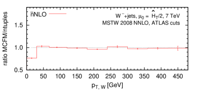
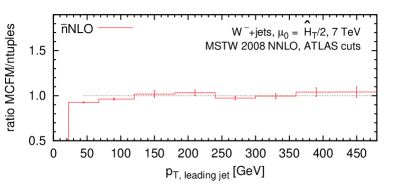
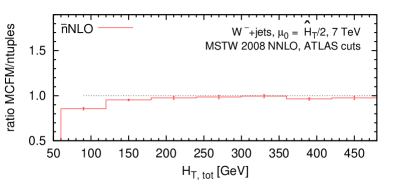
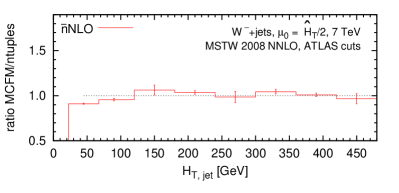
The results for W+jets and Z+jets production at NLO were obtained both with LoopSim+mcfm and with LoopSim+root ntuples. Although the LoopSim method allows in principle to use event samples with arbitrarily low jet transverse momentum, we need to impose a cut on this quantity for efficiency reasons. This technical cut-off on the of jets was set to 1 for mcfm but only 20 for the ntuples. In Fig. 1 we show the effect of this different choice on several distributions. We see that the lack of jets below 20 in the root ntuples has an effect only at low /. Above 100-200 GeV the two approaches give consistent results at NLO. Since its technical cut-off is lower, we shall only show predictions from LoopSim interfaced with mcfm in the following section. The independence on the technical cut-off of the prediction at high transverse momenta is encouraging for the prospect of extending this study to include higher jet multiplicity samples that are available through blackhat+sherpa ntuples. We have verified that all NLO histograms for the observables shown in this study coincide for the mcfm and blackhat+sherpa ntuples except in immediate proximity of the generation cut.
3 results for W/Z+jets at the LHC at 7 TeV
In our computation, at all orders, we used the MSTW NNLO 2008 PDFs [38], with . Jets were obtained from clustering final state partons with the anti- [39] algorithm, using FastJet [32, 33], with the radius . The specific cuts for W+jets and Z+jets processes are given in the corresponding subsections below, and were chosen to match the experimental analyses [3] and [2, 4], respectively. For the central value of the factorization and the renormalization scale, we chose
| (2) |
which is a scalar sum of transverse momenta of all particles in the event, i.e. partons, charged leptons and, if applicable, the neutrino.
The results presented in the following subsections correspond to the parton level. In addition, for the plots with comparisons to the experimental data, and for those plots only, we included the non-perturbative corrections from hadronization and the underlying event, supplied by ATLAS [3, 4]. The cross sections correspond to a single lepton channel and, in the case of W+jets, they include contributions from both W+ and W-.
3.1 W+jets
The analysis is performed with the following cuts [3]: The charged leptons are required to have and . The missing transverse energy must be above . The transverse mass of the W, defined as , is required to be greater than . Only events with jets with and are accepted. In addition, if the distance between a jet and a lepton is smaller than 0.5, this jet is removed from the list of the jets, but the event is kept, as long as the other requirements are met.
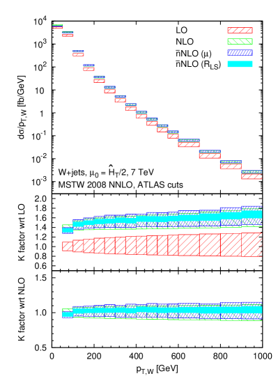
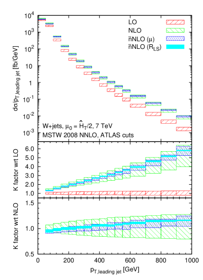
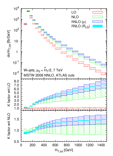
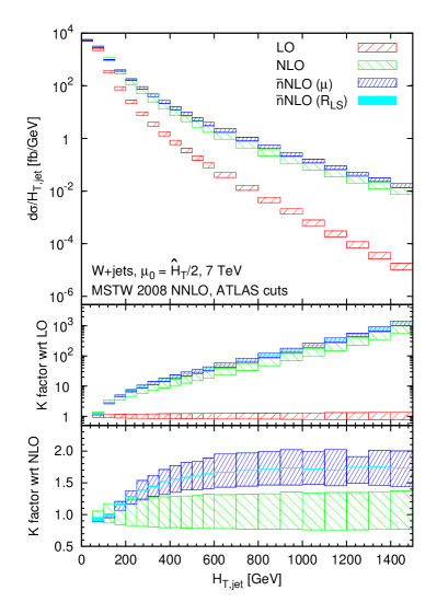
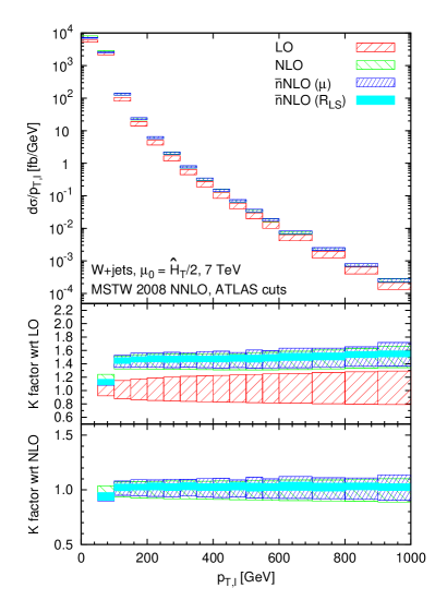
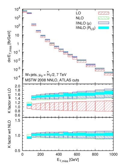
In Figs. 2 and 3, we present the differential distributions for the following observables:
-
•
: transverse momentum of the vector boson,
-
•
: transverse momentum of the hardest jet,
-
•
: sum of the transverse momenta of the leptons (including the neutrino) and jets passing the jet cuts,
-
•
: sum of the transverse momenta of the jets passing the jet cuts.
The predictions are at the pure parton level for . In each plot, the top panel shows the distributions at LO, NLO and NLO whereas the middle and the bottom ones depict the K-factors with respect to LO and NLO.
The distribution of the of the W boson, shown in Fig. 2, is fairly insensitive to new topologies appearing at NLO, and therefore does not exhibit a large NLO/LO K-factor and does not receive significant corrections at NLO. In contrast, the distribution of the of the leading jet from Fig. 2 shows a large K-factor at NLO, which grows with and which arises due to new topologies with soft and collinear W boson. This observable is therefore very suitable for LoopSim predictions at NLO, cf. Eq.(1). Indeed, we see a substantial (almost 70% at high ) reduction of the scale uncertainty at NLO, while the result stays within the NLO band. That indicates that the distribution of the leading jet comes under control at NLO, which matches the expectations, as no new channel or topologies appear at this order. We also note that the uncertainty due to the variation is smaller than the scale uncertainty and it decreases with increasing .
As mentioned in Sec. 2, and explained in more detail in [27], the LoopSim method is expected to give accurate predictions in the region in which a substantial part of the NLO/LO K-factor comes from new channels or new topologies, as opposed to the constant loop terms. As shown in the middle panel of the distribution in Fig. 2, the K-factor, which comes predominantly from genuine loop effects of the LO-type topology diagrams, is around 1.5. Those LO-type topologies should still give significant contributions to the low region of the leading jet distributions and we expect that new topologies start giving the dominant corrections around the K-factor , which corresponds to . Therefore, the NLO result from LoopSim is expected to be accurate above that value of .
Fig. 2 shows also the and distributions. We see that both receive large corrections at NLO reaching above 50% at 1.5 TeV, and lying outside the NLO bands. The reduction of the scale uncertainty at NLO is only minor for these observables, however, do to the 50% increase, the relative scale uncertainty is smaller than that of the NLO result. We also see that the uncertainty is negligible. The large NLO corrections to and come from the third jet, present due to initial state radiation. This jet’s adds a small contribution to but, because the spectrum is steeply falling, the enhancement in the distribution is substantial.
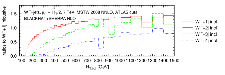
The importance of including higher multiplicities for the description of is illustrated in Fig. 4. One sees that as the value of increases, the NLO prediction for the higher multiplicity increases relative to the inclusive 1-jet contribution, the latter being overtaken by the 2-jet prediction at the value of and by the 3-jet contribution at the value of . This fact demonstrates the need to include higher order effects to describe the distribution. In our calculation we include the 1 and 2-jet contribution at NLO and the 3-jet contribution at LO. We expect the 3 and 4-jet topologies at NLO to play a role above 600 GeV. It would therefore be interesting to study the inclusion of these higher multiplicities, along with a simulated estimate of the corresponding loop effects, using the LoopSim method.
Finally, in Fig. 3, we present the results for the of the lepton and missing transverse energy. Both of these distributions, just like the from Fig. 2 are not sensitive to new topologies appearing at NLO and therefore they are well behaved already at that order. Consequently, the NLO result from LoopSim does not lead to any significant difference with respect to NLO.
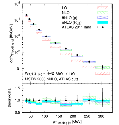
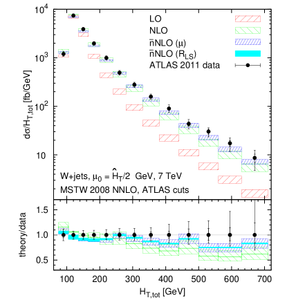
In Fig. 5, we compare our predictions to the existing, , data from ATLAS [3]. Fig. 5 (left) shows the differential distributions for the transverse momentum of the hardest jet and Fig. 5 (right), the scalar sum of the traverse momenta of jets, leptons and missing energy, . The inner and outer bars on the data points correspond to statistical and total error, respectively. The theoretical predictions computed at LO, NLO and NLO orders in QCD were corrected for hadronization and UE effects using the coefficients determined in [3].
The NLO prediction for the distribution of the of the leading jet, stays within the NLO band and its scale uncertainty is significantly reduced with respect to NLO. At low , it touches the lower edge of the NLO band but, as discussed above, this region is potentially sensitive to the genuine constant terms of the loop diagrams, which are not guaranteed to be determined precisely by the LoopSim method. In the case of , the NLO result goes beyond the NLO uncertainty band for and the corrections are up to 30% with respect to NLO. The uncertainty becomes very small above 300 GeV. As we see in Fig. 5 (right), the NLO result, by including configurations with three partons in the final state, describes the data better than the inclusive W+1 jet NLO prediction. It would be interesting to establish whether inclusion of the NLO corrections (i.e. exact 1-loop and simulated 2 and 3-loops) would further improve the agreement with the data. We leave this question for future work.
3.2 Z+jets
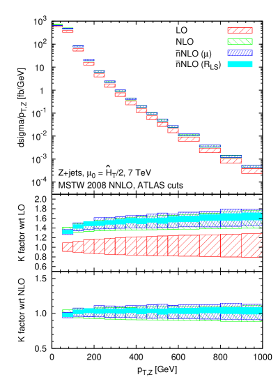
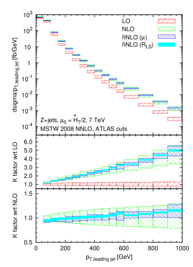
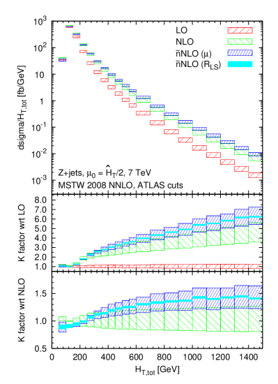
This process involves the production of a Z boson with one or more jets, including the effects of interference with virtual photon. The Z boson subsequently decays into a pair of electrons or muons.
The analysis is performed with the following cuts [2, 4]: The charged leptons are required to have and and the dilepton mass must lie in the window . The jets are required to be sufficiently hard and central with and and, similarly to the W+jets case, they are removed from an event if .
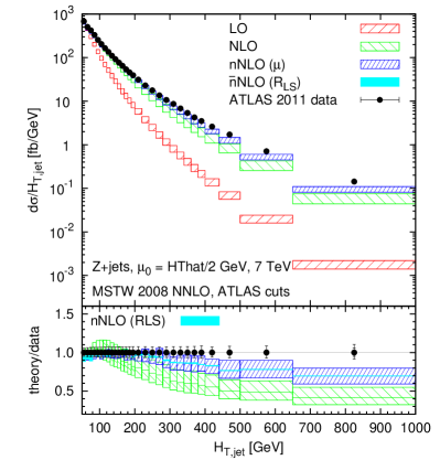
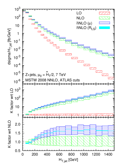
In Fig. 6, we show several distributions relevant for this process. All details are the same as in the W+jets case discussed above. Also, the qualitative behaviour is similar. Thus, the distribution of the of the Z boson does not receive any significant corrections at NLO, which is related to the small NLO/LO K-factor for this observable and to its low sensitivity to new topologies appearing at NLO. 111This does not imply that there are no significant contributions coming from constant terms of the 2-loop diagrams, as we discuss further in this section. On the other hand, the distribution of the of the leading jet is significantly improved at NLO and comes under control at this order. As discussed in the previous subsection, LoopSim becomes powerful in predicting this distribution above . The and distributions receive large, up to 50% corrections at NLO and this, together with the small reduction of scale uncertainties, indicates that they are still not converging at this order due to lacking multiplicities. We also computed the distributions of the of the leading and of the trailing lepton (results not displayed) and, as in the case of the and of the W+jets process, they do not show an improvement at NLO.
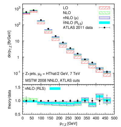
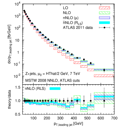
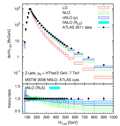
In Fig. 7 we compare our predictions with the ATLAS results obtained at [4]. The distributions correspond to a single lepton channel. The inner and outer bars on the data points correspond to statistical and total error, respectively. The theoretical results at LO, NLO and NLO were corrected for hadronization and UE effects, as well as for QED effects, following the procedure used in [4]. Moreover, in the theory/data ratio, the experimental results were normalized to the inclusive Z cross section, measured in the same fiducial volume whereas the theory results were normalized using an analogous result from blackhat+sherpa.
As expected, the distribution does not receive an improvement at NLO and the offset in the theory/data ratio in the region around , observed at NLO, stays also at NLO. This could, in principle, point to non-negligible constant terms of the 2-loop diagrams. The distribution of the leading jet shows a significant reduction of the scale uncertainty at NLO and a small dependence on at higher values.
The and results at NLO compare significantly better to the experimental data than plain NLO. They quickly go outside of the NLO bands and their scale uncertainty is only moderately reduced.
3.3 Ratios
The productions of +jets and Z+jets bear obviously a number of common features. It is therefore interesting to use the distributions discussed in Sec. 3.1 and 3.2, to form ratios of W+jets/Z+jets and W++jets/W-+jets.222As mentioned earlier, whenever we write “W+jets” we really mean the sum: W++jets + W-+jets. From the theory point of view, such ratios have a number of potential advantages as the dependencies on kinematic variables, scales and PDFs, cancel to a large extent. They are also motivated experimentally since they should be almost free of uncertainties coming from luminosity measurement, jet energy scale or unfolding.
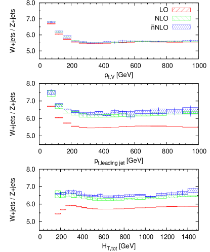
In Fig. 8 (left) we show the W+jets/Z+jets ratios as functions of the of the electroweak boson, of the leading jet and . The bands correspond to varying the renormalization and factorization scale by factors 1/2 and 2, simultaneously for the numerator and the denominator, hence they indicate scale dependence of the ratios. We see that the results are flat, regardless of the order, except for the range below 200 GeV, where the difference between the masses of W and Z is still non-negligible compared to their transverse momenta.
As shown in [40], the production of W+jets at high at LO occurs predominantly via and , for W+ and W-, respectively, whereas for Z+jets it involves both and channels in approximately equal proportions. Therefore, the parton luminosities in the numerator and in the denominator yield a very similar dependence, leading to flat ratios. Similar mechanism is at work for the subdominant channel where W++jets is produced via and W-+jets via , whereas Z+jets production involves the and channels. The and parton distribution functions are, however, very close to each other, which again results in a similar -dependence in the numerator and in the denominator, and hence the flat W+jets/Z+jets ratios. The exact value of the LO ratios from Fig. 8 (left), above 200 GeV, is an overall effect of different decay channels of the W and Z bosons and different cuts used for the two processes.
The situation looks very similar at NLO, where the new production channels, and are the same for the two processes and therefore do not change the results qualitatively. Quantitatively, as expected, since the new NLO channels only moderately modify the distributions, the corresponding NLO ratio from Fig. 8 (left) receives no corrections at this order. On the contrary, these new NLO channels and topologies contribute significantly to the and distributions (cf. Figs. 2 and 6), which, through different cuts on the W and Z bosons decay products, lead to an increase of the ratios.
Finally, the NLO results from Fig. 8 (left) show that the corrections have at most a few percent effect on the ratios, to be compared with up to 50% effect for separate distributions from Figs. 2 and 6. On the top of that, the renormalization and factorization scale dependence, indicated by the widths of the bands shown in Fig. 8, is very weak.
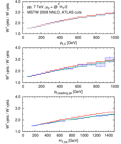
Fig. 8 (right) shows the W++jets/W-+jets ratios and the observations made above largely apply also here. In particular, the NLO and NLO corrections are small and the dependence on the renormalization and factorization scale is significantly lower than for each distribution separately. The W++jets/W-+jets ratios, however, are not flat because they involve the PDF ratio, which is an increasing function of and large values correspond to the tails of the distributions. This observation is consistent with findings from [40].
Altogether, the low sensitivity to higher order QCD corrections and weak dependence on the factorization and renormalization scales make the ratios from Fig. 8 very good observables with great potential to be used in precision studies.
4 Conclusion
We presented the study of W+jets and Z+jets production at the approximate next-to-next-to leading order in QCD. We focused on the center of mass energy and we adopted the fiducial volumes of [3, 4], which allowed for a direct comparison of our results to the available ATLAS data. We used the LoopSim method to merge NLO samples of different multiplicity obtained from mcfm and from blackhat+sherpa in order to compute the dominant part of the NNLO corrections for jet observables at high . Our predictions, referred to as NLO, are expected to be accurate in the regions of phase space dominated by new channels and new topologies appearing at NLO. This corresponds to the large / regions of distributions.
We found that, for both processes, the leading jet distribution comes under control at NLO, with the scale uncertainty being reduced by up to 70% and the result staying within the NLO band. On the contrary, the -type observables still receive significant corrections at NLO, of the order of 50% with respect to NLO. We also checked that, as expected, for the distributions of the of the electroweak bosons, leptons and missing , which do not exhibit a large K-factor at NLO, the NLO result does not bring any significant correction.
For both W+jets and Z+jets processes, we compared our NLO results to the experimental data from ATLAS. For , the agreement between data and theory is comparable to that at NLO. As mentioned above, the NLO result exhibits, however, much smaller theoretical uncertainty. Nevertheless, the statistical errors of the data are still too large at high to favour one prediction of over the other. On the other side, the and distributions at NLO agree much better with the data than NLO. As discussed in Sec. 3.1, this is due to the fact that the NLO result includes V+2j configurations at NLO and V+3j configurations at LO, which represent a sizable contribution at high . It would be interesting to investigate whether the situation improves further at NLO, where the V+4jets configurations would be included. This is left for future work.
The code used in our study is publicly available at:
It contains the LoopSim library together with the interfaces to mcfm 6.6 and to root ntuples. The blackhat+sherpa ntuples will be made available soon and the next version of mcfm 6.7 will include several extra features that will make it easier to interface with LoopSim.
Acknowledgement
We thank Gavin Salam for numerous discussions during this work and for subsequent comments on the manuscript. We are grateful to Ulla Blumenschein and Joey Huston for useful conversations, clarifying a number of experimental issues, and for critical reading of the manuscript. We acknowledge valuable discussions with Stefano Camarda and Nicolas Meric at various stages of this work. We are grateful to Graeme Watt for pointing us to relevant findings concerning ratios of W and Z cross sections. We thank Alberto Guffanti and Pavel Storovoitov for smooth collaboration on the extensions of mcfm, and the mcfm authors for including these new features in the next release. We thank the blackhat+sherpa authors for providing us with the root ntuples. We acknowledge correspondence with Alexander Paramonov concerning experimental details of the W+jets results from ATLAS. DM’s work was supported by the Research Executive Agency (REA) of the European Union under the Grant Agreement number PITN-GA-2010-264564 (LHCPhenoNet).
References
- [1] G. Aad et al. [ATLAS Collaboration], Phys. Rev. D 85 (2012) 012005 [arXiv:1108.6308 [hep-ex]].
- [2] G. Aad et al. [ATLAS Collaboration], Phys. Rev. D 85 (2012) 032009 [arXiv:1111.2690 [hep-ex]].
- [3] G. Aad et al. [ATLAS Collaboration], Phys. Rev. D 85 (2012) 092002 [arXiv:1201.1276 [hep-ex]].
- [4] G. Aad et al. [ATLAS Collaboration], arXiv:1304.7098 [hep-ex].
- [5] S. Chatrchyan et al. [CMS Collaboration], JHEP 1201 (2012) 010 [arXiv:1110.3226 [hep-ex]].
- [6] S. Chatrchyan et al. [CMS Collaboration], Phys. Lett. B 722 (2013) 238 [arXiv:1301.1646 [hep-ex]].
-
[7]
J. M. Campbell and R. K. Ellis,
Phys. Rev. D 60 (1999) 113006
[arXiv:hep-ph/9905386];
J. Campbell, R.K. Ellis, et al. http://mcfm.fnal.gov - [8] J. M. Campbell, R. K. Ellis and D. L. Rainwater, Phys. Rev. D 68 (2003) 094021 [arXiv:hep-ph/0308195].
- [9] R. K. Ellis, K. Melnikov and G. Zanderighi, JHEP 0904, 077 (2009) [arXiv:0901.4101 [hep-ph]]; Phys. Rev. D 80, 094002 (2009) [arXiv:0906.1445 [hep-ph]].
- [10] C. F. Berger, Z. Bern, L. J. Dixon, F. Febres Cordero, D. Forde, H. Ita, D. A. Kosower and D. Maître, Phys. Rev. D 78 (2008) 036003 [arXiv:0803.4180 [hep-ph]]; C. F. Berger, Z. Bern, L. J. Dixon, F. Febres Cordero, D. Forde, T. Gleisberg, H. Ita and D. A. Kosower et al., Phys. Rev. Lett. 106 (2011) 092001 [arXiv:1009.2338 [hep-ph]]; H. Ita, Z. Bern, L. J. Dixon, F. Febres Cordero, D. A. Kosower and D. Maître, Phys. Rev. D 85 (2012) 031501 [arXiv:1108.2229 [hep-ph]]; Z. Bern, L. J. Dixon, F. F. Cordero, S. Hoeche, H. Ita, D. A. Kosower, D. Maître and K. J. Ozeren, arXiv:1304.1253 [hep-ph].
- [11] T. Gleisberg, S. Hoeche, F. Krauss, A. Schalicke, S. Schumann and J. -C. Winter, JHEP 0402 (2004) 056 [hep-ph/0311263]; T. Gleisberg, S. .Hoeche, F. Krauss, M. Schonherr, S. Schumann, F. Siegert and J. Winter, JHEP 0902 (2009) 007 [arXiv:0811.4622 [hep-ph]]; F. Krauss, R. Kuhn and G. Soff, JHEP 0202, 044 (2002) [hep-ph/0109036]; T. Gleisberg and F. Krauss, Eur. Phys. J. C 53, 501 (2008) [arXiv:0709.2881 [hep-ph]].
- [12] J. Alcaraz Maestre et al. [SM AND NLO MULTILEG and SM MC Working Groups Collaboration], arXiv:1203.6803 [hep-ph].
- [13] T. Sjostrand, S. Mrenna and P. Z. Skands, JHEP 0605 (2006) 026 [hep-ph/0603175].
- [14] G. Corcella, I. G. Knowles, G. Marchesini, S. Moretti, K. Odagiri, P. Richardson, M. H. Seymour and B. R. Webber, JHEP 0101 (2001) 010 [hep-ph/0011363].
- [15] M. L. Mangano, M. Moretti, F. Piccinini, R. Pittau and A. D. Polosa, JHEP 0307 (2003) 001 [hep-ph/0206293].
- [16] J. R. Andersen and J. M. Smillie, JHEP 1001 (2010) 039 [arXiv:0908.2786 [hep-ph]]; J. R. Andersen and J. M. Smillie, Phys. Rev. D 81 (2010) 114021 [arXiv:0910.5113 [hep-ph]].
- [17] J. R. Andersen, T. Hapola and J. M. Smillie, JHEP 1209 (2012) 047 [arXiv:1206.6763 [hep-ph]].
- [18] S. Frixione and B. R. Webber, JHEP 0206 (2002) 029 [hep-ph/0204244].
- [19] S. Alioli, P. Nason, C. Oleari and E. Re, JHEP 1006 (2010) 043 [arXiv:1002.2581 [hep-ph]].
- [20] S. Hoeche, F. Krauss, M. Schonherr and F. Siegert, Phys. Rev. Lett. 110 (2013) 052001 [Phys. Rev. Lett. 110 (2013) 052001] [arXiv:1201.5882 [hep-ph]].
- [21] S. Hoeche, F. Krauss, M. Schonherr and F. Siegert, JHEP 1304 (2013) 027 [arXiv:1207.5030 [hep-ph]].
- [22] K. Hamilton, P. Nason and G. Zanderighi, JHEP 1210 (2012) 155 [arXiv:1206.3572 [hep-ph]].
- [23] K. Hamilton, P. Nason, C. Oleari and G. Zanderighi, JHEP 1305 (2013) 082 [arXiv:1212.4504 [hep-ph]].
- [24] R. Frederix and S. Frixione, JHEP 1212 (2012) 061 [arXiv:1209.6215 [hep-ph]].
- [25] L. Lönnblad and S. Prestel, JHEP 1303 (2013) 166 [arXiv:1211.7278 [hep-ph]].
- [26] S. Platzer, arXiv:1211.5467 [hep-ph].
- [27] M. Rubin, G. P. Salam and S. Sapeta, JHEP 1009 (2010) 084.
- [28] S. Camarda, arXiv:1306.2579 [hep-ex].
- [29] F. Campanario and S. Sapeta, Phys. Lett. B 718 (2012) 100 [arXiv:1209.4595 [hep-ph]].
- [30] Y. L. Dokshitzer, G. D. Leder, S. Moretti and B. R. Webber, JHEP 9708 (1997) 001 [arXiv:hep-ph/9707323].
- [31] M. Wobisch and T. Wengler, arXiv:hep-ph/9907280.
- [32] M. Cacciari and G. P. Salam, Phys. Lett. B 641 (2006) 57 [hep-ph/0512210].
- [33] M. Cacciari, G. P. Salam and G. Soyez, http://fastjet.fr/ .
- [34] S. Catani, Y. L. Dokshitzer, M. Olsson, G. Turnock and B. R. Webber, Phys. Lett. B 269, 432 (1991);
- [35] S. D. Ellis and D. E. Soper, Phys. Rev. D 48 (1993) 3160 [hep-ph/9305266].
- [36] J. Alwall, A. Ballestrero, P. Bartalini, S. Belov, E. Boos, A. Buckley, J. M. Butterworth and L. Dudko et al., Comput. Phys. Commun. 176 (2007) 300 [hep-ph/0609017].
- [37] Z. Bern, L. J. Dixon, F. F. Cordero, S. Hoeche, H. Ita, D. A. Kosower and D. Maitre, arXiv:1310.7439 [hep-ph].
- [38] A. D. Martin, W. J. Stirling, R. S. Thorne and G. Watt, Eur. Phys. J. C 63 (2009) 189 [arXiv:0901.0002 [hep-ph]].
- [39] M. Cacciari, G. P. Salam and G. Soyez, JHEP 0804 (2008) 063 [arXiv:0802.1189 [hep-ph]].
- [40] S. A. Malik and G. Watt, arXiv:1304.2424 [hep-ph].