Abstract

Based on Compton scattering and meson photoproduction data the polarizabilities of the nucleon are precisely studied and well understood due to recent experimental and theoretical work using nonsubtracted dispersion relations. The recommended experimental values are $\alpha_{p}=12.0\pm 0.6$, $(12.0)$, $\beta_{p}=1.9\mp 0.6$, $(1.9)$, $\alpha_{n}=12.5\pm 1.7$, $(12.7\pm 0.9)$, $\beta_{n}=2.7\mp 1.8$, $(2.5\mp 0.9)$ in units of $10^{-4}$fm³ and $\gamma^{(p)}_{\pi}=-36.4\pm 1.5$, $(-36.6)$, $\gamma^{(n)}_{\pi}=+58.6\pm 4.0$, $(58.3)$, $(\gamma^{(p)}_{0}=-0.58\pm 0.20)$, $(\gamma^{(n)}_{0}=0.38\pm 0.22)$ in units of $10^{-4}$fm⁴ [1]. The numbers given in parentheses are predicted values. It is shown that all versions of chiral effective field theories applied in analyses of nucleon polarizabilities and Compton scattering ignore essential effects of $\omega$, $\rho$ and $\sigma$ exchanges and of pseudoscalar $\pi$N coupling.

1 Introduction

The description of Compton scattering by the nucleon via dispersion theory was developed at the beginning of the 1960s [2]. The theory made use of relations which may be denoted as $s$-channel dispersion relations and $t$-channel dispersion relations. The singularities entering into the $s$-channel dispersion relations may be taken from meson photoproduction experiments, whereas the singularities entering into the $t$-channel dispersion relations are related to $\pi\pi$ pairs created in two-photon reactions in case of the scalar $t$-channel, and to the $\pi^{0}$ meson in case of the pseudoscalar $t$-channel. The first application of the scalar $t$-channel to the polarizabilities of the nucleon came with the work of J. Bernabeu, T.E.O Ericson et al. (BEFT) in 1974 [3] where it was shown that the largest part of the electric polarizability and the total diamagnetic polarizability are due to the $t$-channel. The smaller part of the electric polarizability is due to the “pion cloud” showing up as a nonresonant meson photoproduction process. The paramagnetic polarizability is mainly due to the photoabsorption cross section provided by the $P_{33}(1232)$ resonance.

A convenient version of a dispersion theory applicable in a wide angular interval and at energies up to 1 GeV was developed by L’vov et al. [4]. This dispersion theory is of the fixed-$t$ variety where $s$-channel integrals are carried out along integration paths at constant $t$, and the $t$-channel contributions are taken care of in the form of “asymptotic” contributions, being an equivalent of the $t$-channel contributions. In principle this version of dispersion theory is completely equivalent to other versions as there are fixed-$\theta$ dispersions theories or hyperbolic dispersion theories. At first sight there appears to be a disadvantage in case of fixed-$t$ dispersion theories because the integration paths are partly located in the unphysical range of the scattering plane. However, it has been shown by L’vov et al. [4] that this only leads to minor technical problems which can be solved without loss of precision. The validity of this latter statement has been clearly demonstrated by experiments, showing that fixed-$t$ dispersion theories lead to a precise representation of the experimental differential cross sections in the whole angular interval and at energies up to 1 GeV [4, 5, 6]. In this respect the nonsubtracted dispersion theory differs from the subtracted dispersion theory [7] which looses validity already at the peak energy of the $\Delta$ resonance. For the spin-independent $t$-channel contribution the assumption was made that it is possible to represent it via a scalar $\sigma$-meson pole-term, in analogy to the well-known pseudoscalar $\pi^{0}$ pole term as entering into spindependent amplitudes. With this representation it was possible to arrive at agreement with experimental data in the angular and energy ranges described above, whereas without this representation of the pole term there remained a large discrepancy between prediction and the experimental data. This implies that at energies of the second resonance region of the nucleon and large scattering angles the $\sigma$-meson pole makes a dominant contribution to the Compton differential cross section. Furthermore, the $\sigma$-meson mass was determined to be $m_{\sigma}=600$ MeV [5, 6] in agreement with other available data. These first investigations published in 2001 [5, 6] remained preliminary because the $\sigma$-meson pole was only an ansatz at that time and there was an uncertainty about its validity. This uncertainty has been removed in later investigations where it was shown that the $\sigma$-meson pole term has a very firm theoretical basis and that the quantitative predictions calculated from well known properties of the $\sigma$-meson are precise (see [1] for a summary). As a conclusion we may state that the dispersion theory of L’vov et al. [4] is precise and well tested. Therefore, there are good reasons to trust in the evaluations of electromagnetic polarizabilities from low-energy Compton-scattering data where use is made of this type of dispersion theory. This is the case for all experimental data which are summarized in [8, 1] leading to the recommended nucleon polarizabilities given in the abstract. For the neutron also electromagnetic scattering of slow neutrons has been taken into account. Furthermore, these recommended values are in excellent agreement with independent predictions obtained from high-precision CGLN amplitudes [9] and well-investigated properties of the $\sigma$ meson without making use of experimental Compton differential cross sections [1].

In addition to dispersion theory $\chi$EFT plays a prominent rôle in current investigations of nucleon Compton scattering and polarizabilities. The present investigation is motivated by the fact that recently $\chi$EFT has been used as a tool for analyses of experimental differential cross sections for Compton scattering by the proton, and results have been obtained which are considerable different from the well-founded standard values $\alpha_{p}=12.0\pm 0.6$ and $\beta_{p}=1.9\mp 0.6$. Examples are the ChPT-investigation of Beane et al. [10] where the values $\alpha_{p}=12.1\pm 1.1\pm 0.5$, $\beta_{p}=3.4\pm 1.1\pm 0.1$ have been obtained, and McGovern et al. [11] where $\alpha_{p}=10.65\pm 0.35\pm 0.36$, $\beta_{p}=3.15\pm 0.35\pm 0.36$ have been obtained. These values have been included in the data listing of the Particle Data Group [12] though the magnetic polarizabilities $\beta_{p}$ of [10, 11] deviate from the respective recommended value [1] by a factor $\sim 1.7$ and the electric polarizability $\alpha_{p}$ of [11] by $\sim 1.7$ standard deviations. These new results are based on the same set of experimental data as the previous ones [1] so that the deviations are solely due to differences in the methods of data analysis. It is obvious that the new analyses are justified only if they are superior to or at least of the same quality as the previous ones. The purpose of the present work is to explore whether or not this is the case.

2 Summary of results of dispersion theory

In a recent article [1] a complete description of the present status of dispersion theory of nucleon Compton scattering and polarizabilities has been given. The recommended experimental polarizabilities introduced in the 2005 summary [8] have been confirmed in the 2013 summary [1] except for a slight correction applied to $\gamma^{(p)}_{\pi}$. The reason for this slight correction was due to the fact that new high-precision analyses of CGLN amplitudes have become available [9] which made this revision necessary. These new high-precision analyses [9] were also of great importance in connection with the prediction of the $s$-channel components of the nucleon polarizabilities for all resonant and nonresonant excitation processes of the nucleon. Results of these analyses which are of interest here are summarized in Table 1.

Table 1: $s$-channel electromagnetic polarizabilities compared with experimental data.

	$\alpha_{p}$	$\beta_{p}$	$\alpha_{n}$	$\beta_{n}$
$s$-channel prediction	$+4.48$	$+9.44$	$+5.12$	$+10.07$
experimental data	$12.0\pm 0.6$	$1.9\mp 0.6$	$12.5\pm 1.7$	$2.7\mp 1.8$
difference line 3 - line 2	$+7.5$	$-7.5$	$7.4$	$-7.4$

As documented in line 4 of Table 1 the $s$-channel predictions show a large deviation from the experimental data and these deviations are the same for the proton and the neutron. Furthermore, the differences obtained for the electric and the magnetic polarizabilities given in line 4 only differ by the signs. This means that these differences cancel in case of $\alpha+\beta$, i.e. $(\alpha+\beta)^{t}\equiv 0$, but make a dominant contribution, viz. $(\alpha-\beta)^{t}$, in case of $\alpha-\beta$.

As has been pointed out in [1] the $t$-channel contribution differs from the $s$-channel contribution due to the fact that the former can be traced back to the mesonic structure of the constituent quarks. This means that the short-distance contribution [13] introduced in some versions of $\chi$EFT may tentatively also be viewed in terms of properties of the constituent quarks. In spite of this interesting similarity there is an essential difference between $\chi$EFT and dispersion theory due to the fact that dispersion theory provides a method for a quantitative prediction of the $t$-channel contribution, whereas the $\chi$EFT prediction for the short-distance contribution is treated as an adjustment, filling the gap between predictions and experimental data. This is the reason for naming them counterterms (c.t.) with $\delta\alpha$ corresponding to the electric part and $\delta\beta$ corresponding to the magnetic part.

2.1 Quantitative prediction of the $t$-channel component

The $t$-channel component of the electromagnetic polarizabilities of the nucleon has been first described by J. Bernabeo, T.E.O. Ericson et al (BEFT) [3] in the following way: If we restrict ourselves in the calculation of the $t$-channel absorptive part to intermediate states with two pions with angular momentum $J\leq 2$, the sum rule takes the convenient form for calculations [3]:

$$(\alpha-\beta)^{t} = \frac{1}{16\pi^{2}}\int^{\infty}_{4m^{2}_{\pi}}\frac{dt}{t^{2}}\frac{16}{4m^{2}-t}\left(\frac{t-4m^{2}_{\pi}}{t}\right)^{1/2}\Big{[}f^{0}_{+}(t)F^{0*}_{0}(t)$$ (1)

$$-\left(m^{2}-\frac{t}{4}\right)\left(\frac{t}{4}-m^{2}_{\pi}\right)f^{2}_{+}(t)F^{2*}_{0}(t)\Big{]},$$

where $f^{(0,2)}_{+}(t)$ and $F^{(0,2)}_{0}(t)$ are the partial-wave helicity amplitudes of the processes $N\bar{N}\to\pi\pi$ and $\pi\pi\to\gamma\gamma$ with angular momentum $J=0$ and $2$, respectively, and isospin $I=0$. Though being the first who published the BEFT sum rule in its presently accepted form, Bernabeu and Tarrach [3] were not aware of the appropriate amplitudes to calculate the BEFT sum rule numerically. Later on evaluations of Eq. (1) also remained rather uncertain until recently, when Drechsel et al. [7] and Levchuk [14] carried out calculations with good precision.

Table 2: Numerical evaluation of the BEFT sum rule and of the equivalent $\sigma$-meson pole.

$(\alpha_{p}-\beta_{p})^{t}$	authors & methods
$+16.5$	Drechsel,Pasquini, Vanderhaeghen,2003[7], (Eq. 1)
$+14.0$	Levchuk, 2004 [14], (Eq. 1)
$+15.2$	prediction based on the $\sigma$-meson pole [1], (Eq. 5)

The results obtained in this way are listed in lines 2 and 3 of Table 2. In the $t$-channel notation the two-photon process described by Eq. (1) may be written in the form

$$\gamma\gamma\to\sigma\to\pi\pi\to\sigma\to N\bar{N},$$ (2)

i.e. by a pion pair in the intermediate state, coupled to two photons on the one hand and to a $N\bar{N}$ pair on the other, via correlations which may be understood as $\sigma$ mesons. As has been justified in detail in [1] this composite intermediate state can be replaced by

$$\gamma\gamma\to\sigma\to N\bar{N}$$ (3)

which describes the $t$-channel pole contribution in complete analogy to the well known $\pi^{0}$ pole contribution

$$\gamma\gamma\to\pi^{0}\to N\bar{N}.$$ (4)

This leads to the prediction derived in [15, 16]

$$(\alpha-\beta)^{t}=\frac{g_{\sigma NN}{\cal M}(\sigma\to\gamma\gamma)}{2\pi m^{2}_{\sigma}}+\frac{g_{f_{0}NN}{\cal M}(f_{0}\to\gamma\gamma)}{2\pi m^{2}_{f_{0}}}+\frac{g_{a_{0}NN}{\cal M}(a_{0}\to\gamma\gamma)}{2\pi m^{2}_{a_{0}}}\tau_{3},$$ (5)

where the $\sigma$-meson part is given by

$$(\alpha-\beta)^{t}_{\sigma}=\frac{5\alpha_{em}g_{\pi NN}}{6\pi^{2}m^{2}_{\sigma}f_{\pi}}=15.2$$ (6)

with $\alpha_{em}=1/137.04$, $g_{\sigma NN}\equiv g_{\pi NN}=13.169\pm 0.057$, $f_{\pi}=(92.42\pm 0.26)$ MeV, $m_{\sigma}=666$ MeV, as derived in [17] and given in line 4 of Table 2. Now with $(\alpha+\beta)^{t}=0$ we arrive at

$$\alpha^{t}=+\frac{1}{2}(\alpha-\beta)^{t}=+7.6\,\,\,(\sim 62\%\,\,\,{\rm of}\,\,\,\alpha),$$ (7)

$$\beta^{t}=-\frac{1}{2}(\alpha-\beta)^{t}=-7.6\,\,\,(100\%\,\,\,{\rm of}\,\,\,\beta_{\rm dia})$$ (8)

in excellent agreement with the findings in Table 1. It should be noted that the largest part of the electric polarizability $\alpha$ (63% for the proton and 61% for the neutron) and 100% of the diamagnetic polarizability $\beta_{\rm dia}$ are due to the $t$-channel.

The contributions from the $f_{0}(980)$ and $a_{0}(980)$ scalar meson entering into Eq. (5) are discussed in detail in [1]. These contributions are small and may be represented by

$$\alpha(f_{0}(980),a_{0}(980))=\pm(+0.3-0.4\,\tau_{3}).$$ (9)

The double, $\pm$, sign on r.h.s. of Eq. (9) indicates that we leave the sign of $\alpha(f_{0}(980),a_{0}(980))$ undetermined and, as a consequence, include this quantity into the error when calculating the neutron electromagnetic polarizability $\alpha_{n}$ from the experimental proton electric polarizability $\alpha_{p}$ and the predicted difference $(\alpha_{n}-\alpha_{p})$, leading to [1]

$$\alpha_{n}=12.7\pm 0.9,\quad\beta_{n}=2.5\mp 0.9.$$ (10)

The errors given in (10) take into account the experimental error of $\alpha_{p}$ and the error due to the $t$-channel contributions of the $f_{0}(980)$ and $a_{0}(980)$ scalar mesons. The error of $\alpha_{p}$ is a measure of the precision of the procedure in general and the error of the $f_{0}(980)$ and $a_{0}(980)$ contributions a measure of an additional uncertainty in case of the neutron. This result for the neutron polarizabilities is extremely important because it rests on very firm arguments for the $t$-channel component and on very precise experimental data for the CGLN amplitudes. We propose to use the prediction given in (10) as a benchmark for future high-precicion experiment on the neutron.

The conclusion we may draw from this result is that dispersion theory provides us with a quantitative prediction of the three components of the electromagnetic polarizabilities, as there are the $s$-channel nonresonant and $s$-channel resonant excitations of the nucleon, and the $t$-channel part which may be understood as scattering by the $\sigma$ meson while being part of the structure of the constituent quark. This latter process is expected to take place because the $\sigma$ meson mediates the generation of mass of the constituent quark via chiral symmetry breaking and, therefore, has to be a part of the constituent-quark structure. This very consistent result obtained from dispersion theory contrasts with the unspecified short-distance contribution discussed in case of $\chi$EFT.

2.2 Dependence of the polarizabilities on the photon energy

Compton scattering experiments aimed to determine the polarizabilities of the nucleon are carried out typically at energies above 50 MeV up to energies well below the $\Delta$ peak. In the upper part of this energy interval fits to the experimental differential cross sections require a general knowledge of the photon-energy, $\omega$, dependences of the polarizabilities. Dispersion relations evaluated in the backward direction at $\theta=\pi$ are the appropriate tool to determine these $\omega$ dependences. Figure 1 shows the result of the calculation when including the empirical $E_{0+}$ CGLN amplitude, the $P_{33}(1232)$ resonance and the $\sigma$-meson pole contribution. The latter contribution has been calculated for the mass $m_{\sigma}=600$ MeV. This mass is the appropriate value because it fits the experimental differential cross sections in the second resonance region of the proton. The dispersion relation used for these calculations may be found in [1].

It may be of interest to disentangle the curves shown in Figure 1 into an electric part and a magnetic part. The results obtained are shown in Figure 2.

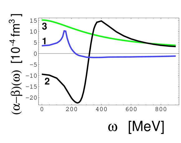
Figure 1: Real part of the three main components of $(\alpha-\beta)(\omega)$ for the proton. 1) Meson-cloud component as given by the $E_{0+}$ CGLN amplitude. 2) Resonant component due to the $P_{33}(1232)$ nucleon resonance. 3) $t$-channel component as given by the $\sigma$-meson pole. The curve is calculated for the $\sigma$-meson mass $m_{\sigma}=600$.

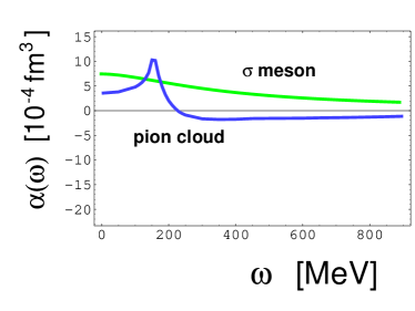
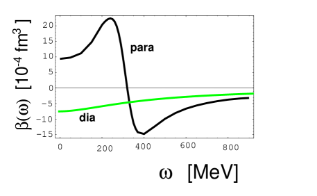
Figure 2: Left panel: Energy dependent electric polarizability $\alpha(\omega)$ due to the pion cloud and the $\sigma$-meson pole (see Fig. 1). Right panel: Energy dependent magnetic polarizability $\beta(\omega)$ due to the $P_{33}(1232)$ resonance and the $\sigma$-meson pole (see Fig. 1).

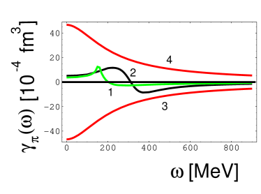
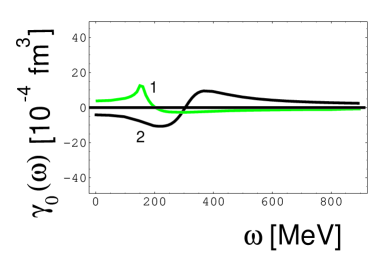
Figure 3: Photon-energy dependent spinpolarizabilities. Left panel: Components of backward spinpolarizabilities, 1) $E_{0+}$ component, 2) $P_{33}(1232)$ component, 3) $\pi_{0}$-pole component for the proton, 4) $\pi_{0}$-pole component for the neutron. Right panel: Components of forward spinpolarizabilities, 1) $E_{0+}$ component, 2) $P_{33}(1232)$ component

.

The $\omega$-dependent electric polarizability as shown in the left panel of Figure 2 is a superposition of the $E_{0+}$ contribution as given by the nonresonant photoabsorption cross section and a positive part of the $\sigma$-meson pole contribution. In a similar way the magnetic polarizability as shown in the right panel of Figure 2 can be traced back to the $P_{33}(1232)$ resonance as the main component of the paramagnetic polarizability, and a negative part of the $\sigma$-meson pole contribution which represents the diamagnetic polarizability.

For sake of completeness we also investigate the $\omega$ dependencies of the spinpolarizabilities. In the left panel of Figure 3 the components of the backward spinpolarizability are shown. There is a constructive interference of the $E_{0+}$ component (curve 1) and the $P_{33}(1232)$ component (curve 2). The main components are due to the $\pi^{0}$ $t$-channel which lead to a destructive interference in case of the proton and to a constructive interference in case of the neutron. In case of the forward spinpolarizability as shown in the right panel of Figure 3 the $E_{0+}$ component (curve 1) and the $P_{33}(1232)$ component (curve 2) interfere destructively. This leads to very small values for the forward spinpolarizabilities for the proton as well as for the neutron. Furthermore, since the $E_{0+}$ component is larger for the neutron than for the proton, whereas the $P_{33}(1232)$ components are the same, it is not a surprise that the forward spinpolarizabilities of the proton and neutron have different signs (see [1] and references therein).

3 Outlook on chiral perturbation theory

Even though QCD is the correct theory for the strong interactions, it cannot easily be used for computations at all energy and momentum scales. At energies of the order of the nucleon mass the Nambu–Jona-Lasinio (NJL) model [18, 19, 20, 21, 22] works extremely well. In addition, the Linear $\sigma$ Model (L$\sigma$M) [23, 24] may be applied where the aspect of spontanous symmetry breaking is exploited. For practical applications it is convenient to make use of the Quark-Level Linear $\sigma$ Model (QLL$\sigma$M) [25] which combines properties of the two models, NJL and L$\sigma$M. For the special problem of nucleon polarizabilities the QLL$\sigma$M of course cannot be applied to the prediction of the polarizabilities in general, but it is very useful and extremely precise to make predictions on the basis of the QLL$\sigma$M for the $t$-channel component [1]. The $s$-channel component can only be reliably predicted on the basis of photomeson data by applying dispersion relations. This has been described in detail in the foregoing section.

Chiral perturbation theory dates back to a paper of Steven Weinberg [26] which is concerned with phenomenological Lagrangians. In this work, for simplicity, Weinberg “integrates out” whatever other degrees of freedom may be present - nucleon, $\rho$ meson, $\sigma$ meson, etc. - and he considers only pions. Furthermore, the derivative (pseudovector) coupling of the pion is introduced as a desired property of the theory.

In case of Compton scattering by the nucleon Weinberg’s concept is applied to the $N\pi$-system [27, 28]. Later on the $\Delta$, $\Delta\pi$ and short-distance degrees of freedom were also taken into account.

3.1 Chiral perturbation theory and the ${\bf E_{0+}}$ CGLN amplitude

In 1993 A. I. L’vov published a paper [29] with the title “A dispersion look at the chiral perturbation theory. Nucleon electromagnetic polarizabilities”. In this paper it is shown that chiral perturbation theory (ChPT) as discussed at that time [27, 28] corresponds to dispersion theory applied to the photomeson $E_{0+}$ CGLN amplitude in the Born approximation. The results obtained are

$$\alpha^{\rm pion\,Born}_{p}=7.3,\quad\beta^{\rm pion\,Born}_{p}=-1.8,\quad\alpha^{\rm pion\,Born}_{n}=9.8,\quad\beta^{\rm pion\,Born}_{n}=-0.9$$ (11)

in very good agreement with the prediction of ChPT [28] as given in the second line of Table 3. By the same procedure the results of the heavy baryon version (HBChPT) have been reproduced by making use the shift $m_{p}\to\infty$ in appropriate parts of the calculation. The numerical results obtained in the HBChPT are given in the third line of Table 3.

Table 3: Predicted electromagnetic polarizabilities of the nucleon compared with experimental data. The predictions given in lines 2 and 3 correspond to ChPT and HBChPT, respectively, the prediction in line 4 to the empirical $E_{0+}$ CGLN amplitude.

	$\alpha_{p}$	$\beta_{p}$	$\alpha_{n}$	$\beta_{n}$
ChPT	7.4	$-2.0$	10.1	$-1.2$
HBChPT	12.6	1.3	12.6	1.3
Empirical $E_{0+}$	3.2	$-0.3$	4.1	$-0.4$
Experiment	$12.0\pm 0.6$	$1.9\mp 0.6$	$12.5\pm 1.7$	$2.7\mp 1.8$

The result obtained by L’vov [29] has been confirmed by the present author in [30] by the following independent procedure. The photoabsorption cross-sections for the $E_{0+}$ CGLN amplitude has been calculated in the Born approximation and on the basis of empirical data as shown in Figure 4. Then dispersion theory has been applied to calculate the corresponding contributions to the electric polarizabilities of the proton and the neutron. The appropriate formulae may be found in [1].

Figure 4: Photoabsorption cross section $\sigma(E_{0+})$ due to $s$-wave single-pion photoproduction for the proton (p) and the neutron (n). The two upper curves have been calculated in the Born approximation. The two lower curves are empirical results [9, 31, 32].

The results obtained in the Born approximation are

$$\alpha^{E_{0+}\,{\rm Born}}_{p}=7.5,\quad\beta^{E_{0+}\,{\rm Born}}_{p}=-1.4,\quad\alpha^{E_{0+}\,{\rm Born}}_{n}=9.9,\quad\beta^{E_{0+}\,{\rm Born}}_{n}=-1.8$$ (12)

and again are in excellent agreement with the data given line 2 of Table 3. This means that the equivalence of the ChPT prediction and the Born approximation found by L’vov [29] has been confirmed. By the same procedure the polarizabilities are also calculated from the empirical $E_{0+}$ amplitudes shown in Figure 4. These results are given in line 4 of Table 3.

When comparing the predictions for the polarizabilities given in Table 3 provided by the empirical $E_{0+}$ CGLN amplitude and the corresponding Born approximation, denoted ChPT, it is of interest to go to Figure 4. Both representations have in common that the cross sections and, therefore, also the electric polarizabilities for the neutron are larger than those for the proton. The reason for this is that the $n\to p\pi^{-}$ transition leads to a larger electric dipole moment than the $p\to n\pi^{+}$ transition [30]. Two reasons for the deviations of the empirical $E_{0+}$ amplitude from the Born approximation have been discussed in [32]. The first reason is that the pseudovector (PV) coupling as entering into the Born approximation is not valid at high photon energies but has to be replaced by some average of PV and pseudoscalar (PS) coupling. The second reason are $\rho$- and $\omega$-meson exchanges which are not taken into account in the Born approximation. It is apparent that the degrees of freedom leading to the large difference between the empirical $E_{0+}$ CGLN amplitudes and the Born approximation are among those which are explicitly “integrated out” in Weinberg’s approach. Furthermore, the use of the derivative PV coupling alone does not lead to the correct results for the cross sections and, therefore, also not for the polarizabilities.

The remarkable agreement of the predictions based on the two versions of chiral perturbations theory with the experimental data may lead to the conclusion that these predictions essentially contain a complete description of the polarizabilities and only need some minor corrections in order to arrive at the final theoretical prediction of the electromagnetic polarizabilities [27, 28]. This conclusion apparently is not correct. In a later versions of chiral perturbation theory [33, 34] which are considered in the next subsections in more detail it was recognized that the resonant excitation of the nucleon plays a dominant rôle and provides a large paramagnetic component. Furthermore, quantities $\delta\alpha$ and $\delta\beta$ denoting the electric and the magnetic counterterms (c.t.), respectively, have been introduced. These counterterms are also denoted short-distance contributions to nucleon polarizabilities [33].

3.2 Chiral dynamics in low-energy Compton scattering off the nucleon versus dispersion theory

For a comparison with dispersion theory (DR) as outlined in the foregoing and in [1] we start with the work of Hildebrandt et al. [33] from the following reasons. This work takes into account a complete list components and provides numerical results for them. These components are
(i) the nonresonant N$\pi$ component which is known to have the $E_{0+}$ CGLN amplitudes as the main part,
(ii) the short-distance or counterterm (c.t.) component which may tentatively be compared with the $t$-channel component of DR,
(iii) the $\Delta$-pole component calculated by the small scale expansion (SSE) method, which may be compared with the resonant $s$-channel component of DR, and
(iv) the $\Delta\pi$ component which may be compared with the $\gamma\to\pi\Delta\to N\pi\pi$ component of the photoabsorption cross section.

Table 4: Components contributing to the electromagnetic polarizabilities of the proton obtained in the SSE-version of HBChPT compared with dispersion theory (DR) as outlined in the foregoing sections and in [1]. The $t$-channel components of DR are tentatively compared with the electric, $\delta\alpha$, and magnetic, $\delta\beta$, counterterm (c.t.).

$\alpha_{p}$	HBChPT	DR	$\beta_{p}$	HBChPT	DR
N$\pi$	+11.87	+3.09	N$\pi$	+1.25	+ 0.48
c.t.	-5.92	+7.6	c.t.	-10.68	-7.6
$\Delta$-pole	0.0	-0.01	$\Delta$-pole	+11.33	+8.56
$\Delta\pi$	+5.09	+1.4	$\Delta\pi$	+0.86	+ 0.4
	11.04	12.08		2.76	1.84

For the N$\pi$ component of $\alpha_{p}$ given in line 2 of Table 4 we find a remarkable discrepancy between the results obtained by the HBChPT-SSE calculation and the results obtained by dispersion theory (DR), amounting to a factor 3.8. This factor is due to the fact that HBChPT replaces the empirical $E_{0+}$ CGLN amplitude by a modified version of the Born approximation which leads to this large factor as discussed in the foregoing subsection.

The counterterms (c.t.) $\delta\alpha$ and $\delta\beta$ given in line 3 of Table 4 are not obtained by a parameter-free prediction, but by adjustments to experimental data. A disadvantage of the result obtained is that the sum $\delta\alpha+\delta\beta$ is unequal to zero and negative. Then, according to Baldin’s sum rule there should be a negative component in the total photoabsorption cross section of the nucleon which is related to this quantity $\delta\alpha+\delta\beta$. Such a component does not exist. On the other hand the predictions in line 3 of Table 4 obtained from the $\sigma$-meson pole term of the $t$-channel (columns DR) obey the condition $\alpha^{t}+\beta^{t}=0$.

The paramagnetic polarizability given in line 4 of Table 4 shows that the SSE-method leads to the right order of magnitude for this quantity. The deviation from the prediction obtained via dispersion theory amounts to 32%.

This is different for the $\Delta\pi$ component which is too big by a factor of 3.6 in case of the electric polarizability and by a factor of 2 in case of the magnetic polarizability. In this case similar effects may play a rôle as in case of the N$\pi$ component.

Summarizing it may be stated that the HBChPT-SSE version of chiral perturbation theory as discussed in this sections has the advantage of containing all the degrees of freedom which also are expected from the point of view of dispersion theory. There is the nonresonant N$\pi$ component, a formal analog (c.t.) of the $t$-channel component, a component from resonant excitation of the nucleon and a $\Delta\pi$ component. However, the numbers obtained certainly need improvements.

3.3 Different variants of chiral EFT

After the first papers on the polarizabilities of the nucleon based on chiral EFTs had been published [27, 28], a large numbers of further papers appeared, revealing agreement and controversies between the methods applied by different groups. In this connection a recent topical review may be cited [35] which covers a major fraction of the development. For the purpose of the present work an other recent paper is of importance [34] which gives, in a concise way, a deeper insights into the methodology of ChPT.

One interesting piece of information is given in terms of counterterms (c.t.) $\delta\alpha^{(p)}_{E1}$ and $\delta\beta^{(p)}_{M1}$ entering into the different variants of chiral EFT. These are given in line 3 of the following Table 5 together with other contributions.

Table 5: Values for the nonresonant N$\pi$ contribution, the counterterm (c.t.), the $\Delta$ pole and the $\Delta\pi$ contribution to the electric $\alpha$ and magnetic $\beta$ polarizabilities in different variants of $\chi$EFT considered in [34]

	I $\alpha$	I $\beta$	II $\alpha$	II $\beta$	III $\alpha$	III $\beta$	IV $\alpha$	IV $\beta$	V $\alpha$	V $\beta$	VI $\alpha$	VI $\beta$
N$\pi$	0.0	0.0	0.0	0.0	12.6	1.3	6.9	-1.8	12.6	1.3	6.9	-1.8
c.t.	10.5	2.7	10.6	-4.4	-2.1	1.4	3.6	4.5	-9.8	-7.1	-0.8	-1.2
$\Delta$ pole	0.0	0.0	-0.1	7.1	0.0	0.0	0.0	0.0	-0.1	7.1	-0.1	7.1
$\Delta\pi$	0.0	0.0	0.0	0.0	0.0	0.0	0.0	0.0	7.8	1.4	4.5	-1.4

The variants considered in [34] are as follows:
I: The results for Compton scattering with nucleon and $\pi^{0}$ Born graphs (Tree graphs), plus polarizabilities as given by the counterterm (c.t.).
II: Tree graphs plus the effects of the (dressed) $\Delta$ $s$- and $u$-channel pole graphs.
III: Tree graphs plus $\pi$N loops: the $O(e^{2}\delta^{2})$ calculation in heavy-baryon $\chi$EFT without an explicit $\Delta$ degree of freedom.
IV: as (III) but with relativistic nucleon propagator in the $\pi$N and $\pi\Delta$ loops.
V: the $O(e^{2}\delta^{3})$ calculation in heavy-baryon $\chi$EFT with explicit $\Delta$, including tree graphs, $\Delta$ poles and HB $\pi$N and $\pi\Delta$ loops.
VI: as (V), but with relativistic nucleon propagators in the $\pi$N and $\pi\Delta$ loops.

According to the authors [34] all of these variants of $\chi$EFT are based on the same low-energy symmetries of QCD and in this sense are equivalent. But only the last two versions V and VI in Table 5 are realistic calculations which can be compared with experimental Compton differential cross sections in the resonance region and some way below. A comparison with experimental data at angles from $\theta_{\rm lab}=60^{\circ}$ to $135^{\circ}$ shows that these two variants of $\chi$EFT which both include the leading $\pi$N loop effects and an explicit $\Delta$ are quite similar, provided the counterterms (c.t.) are included and adjusted to yield identical values for the scalar dipole polarizabilities. However, the values found for the two sets of counterterms in the $\chi$EFT variants considered here are rather different. They are particularly large in the $\pi^{\rm HB}\Delta$ calculation (column V) , especially as compared to the relativistic $\pi\Delta$ one (column VI).

The statements of the authors [34] cited in the forgoing paragraph indicate that in case of $\chi$EFTs a major part of the interest is directed to the low-energy symmetries of QCD, whereas the precision of the numbers attributed to the different components of the polarizabilities is of secondary importance. This attitude contrasts with the aim of the non-subtracted dispersion theory where methods have been developed which lead to a high precision of the different components of the polarizabilities. For the data analysis certainly high precision is required.

4 Discussion and conclusions

(i) The analysis of Compton scattering and polarizabilities in terms of nonsubtracted dispersion relations is precise and well tested experimentally in a large angular range and at energies up to 1 GeV. In this respect the nonsubtracted dispersion theory differs from the subtracted dispersion theory [7] where the latter looses validity already at the peak energy of the $\Delta$ resonance.
(ii) The polarizabilities of the nucleon are determined from experimental data in two ways, firstly by adjusting the predictions of the nonsubtracted dispersion theory to the experimental differential cross sections for Compton scattering in the low-energy domain below the $P_{33}(1232)$ peak and secondly by calculating them from the $s$-channel and $t$-channel singularities as provided by high-precision analyses of CGLN amplitudes and well known properties of the scalar $t$-channel. In the latter case no use is made of Compton scattering differential cross sections. The results obtained by these two methods are in excellent agreement with each other.

The paper of Beane et al. [10] cited in the Introduction is essentially of the variety III in Table 5. The amplitude for unpolarized Compton scattering is expanded in powers of the parameter $Q$ used in EFTs, representing a typical external momentum. To ${\cal O}(Q^{3})$ the polarizabilities are given by pion-loop effects and lead to the HBChPT prediction. At ${\cal O}(Q^{4})$ there are new long-range contributions to these polarizabilities. Four new parameters also appear which encode contributions of short-distance physics to the spin-independent polarizabilities. Thus one needs four pieces of experimental data to fix these four short-distance contributions. After these adjustment to experimental data have been carried out good fits to experimental differential cross sections have been obtained. The paper of Mc Govern et al. [11] cited in the Introduction includes effects of the $\Delta$-resonance and, therefore, essentially is of the variety V in Table 5.

The foregoing analysis has shown that by “integrating out” $\rho$- and $\omega$- degrees of freedom and by using the derivative coupling alone, the $N\pi$ component of the electric polarizability predicted by ChPT is increased by a factor $\sim 2.4$ compared to the correct empirical value. Furthermore, by carrying out the kinematical modifications entering into HBChPT a further increase by a factor of 1.7 (proton) and 1.2 (neutron) is obtained. The “integrating out” of the $\sigma$-meson leads to the omission of the major part, $\alpha^{t}=+7.6$, of the electric polarizability and to the omission of the diamagnetic polarizability $\beta^{t}=-7.6$.

References

- [1] M. Schumacher, M.D. Scadron, Fortschr. Phys. 61 (2013) 703, arXiv:1301.1567 [hep-ph].
- [2] A.C. Hearn, E. Leader, Phys. Rev. 126 (1962) 789; R. Köberle, Phys. Rev. 166 (1968) 1558.
- [3] J. Bernabeu, T.E.O Ericson, C. Ferro Fontan, Phys. Lett. 49 (1974) B 381; J. Bernabeu, B. Tarrach, Phys. Lett. 69 B (1977) 484.
- [4] A.I. L’vov, V.A. Petrun’kin, M. Schumacher, Phys. Rev. C 55 (1997) 359.
- [5] G. Galler et al., Phys. Lett. B 503 (2001) 245.
- [6] S. Wolf et al., Eur. Phys. J. A 12 (2001) 231.
- [7] D. Drechsel, B. Pasquini, M. Vanderhaeghen, Phys. Rept. 378 (2003) 99, arXiv:hep-ph/0212124.
- [8] M. Schumacher, Prog. Part. Nucl. Phys. 55 (2005) 567, [hep-ph/0501167].
- [9] D. Drechsel, S.S. Kamalov, L. Tiator, Eur. Phys. J. 34 (2007) 69, arXiv:0710.0306 [nucl-th].
- [10] S. R. Beane, M. Malheiro, J.A. McGovern, D.R. Phillips, U. van Kolck, Phys. Lett. B 567 (2003) 200; Erratum: Phys. Lett. B 607 (2005) 320, arXiv:nucl-th/0209002.
- [11] J.A. McGovern, D.R. Phillips, H.W. Griesshammer, Eur. Phys. J. A 49 (2013) 12, arXiv:1210.4104 [nucl-th].
- [12] J. Beringer, et al. (Particle Data Group) Phys. Rev. D 86 (2012) 010001 and partial update for the 2014 edition.
- [13] A.I. L’vov, S. Scherer, B. Pasquini, C. Unkmeir, D. Drechsel, Phys. Rev. C 64 (2001) 015203, arXiv:hep-ph/0103172.
- [14] M.I. Levchuk, private communication (2004).
- [15] M. Schumacher, Eur. Phys. J. A 34 (2007) 293, arXiv:0712.1417 [hep-ph].
- [16] M. Schumacher, Nucl. Phys. A 826 (2009) 131, arXiv:0905.4363 [hep-ph].
- [17] M. Schumacher, Eur. Phys. J. A 30 (2006) 413, Erratum 32 (2007) 121, [hep-ph/0609040]; M.I. Levchuk, A.I. L’vov, A.I. Milstein, M. Schumacher, Proceedings of the Workshop on the Physics of Excited Nucleons, World Scientific, NSTAR 2005 (2005) 389, [hep-ph/0511193].
- [18] Y. Nambu, G. Jona-Lasinio, Phys. Rev. 122 (1961) 345.
- [19] U. Vogl, W. Weise, Prog. Part. Nucl. Phys. 27 (1991) 195.
- [20] S. P. Klevansky, Review of Modern Physics 64 (1992) 649.
- [21] Tetsuo Hatsuda, Teiji Kunihiro, Physics Reports 247 (1994) 221.
- [22] Johan Bijnens, Physics Reports 265 (1996) 369.
- [23] M. Gell-Mann, M. Levy, Nuovo Cim. 16 (1960) 705.
- [24] V. de Alfaro, S. Fubini, G. Furlan, C. Rosetti, in Currents in Hadron Physics (North-Holland Publ. Amsterdam, 1973) chap.5.
- [25] M.D. Scadron, G. Rupp, R. Delbourgo, Fortschr. Phys. 61 (2013) 994, arXiv:1309.5041 [hep-ph].
- [26] Steven Weinberg, Physica 96A (1979) 327.
- [27] V. Bernard et al., Phys. Rev. Lett. 67 (1991) 1515.
- [28] V. Bernard et al., Nucl. Phys. B 373 (1992) 346.
- [29] A.I. L’vov, Phys. Lett. B 304 (1993) 29.
- [30] M. Schumacher, Eur. Phys. J. A 31 (2007) 327, arXiv:0704.0200 [hep-ph].
- [31] D. Hanstein, D. Drechsel, L. Tiator, Nucl. Phys. A 632 (1998) 561.
- [32] D. Drechsel, O. Hanstein, S.S. Kamalov, L. Tiator, Nucl. Phys. A 645 (1999) 145.
- [33] R. P. Hildebrandt, et al., Eur. Phys. J. A 20 (2004) 293, [nucl.-th/0307070]
- [34] V. Lensky, J. M. McGovern, D. R. Phillips, V. Pascalutsa, Phys. Rev. C 86 (2012) 048201, arXiv:1208.4559 [nucl-th].
- [35] H. W. Griesshammer, J. A. McGovern, D. R. Phillips, G. Feldman, Prog. Part. Nucl. Phys. 67 (2012) 841, arXiv:1203.6834 [nucl-th].