On the mechanical stability of asymptotically flat black holes
with minimally coupled scalar hair

Abstract

We show that the asymptotically flat hairy black holes, solutions of the Einstein field equations minimally coupled to a scalar field, previously discovered by one of us, present mode instability against linear radial perturbations. It is also shown that the number of unstable modes is finite and their frequencies can be made arbitrarily small.

I Introduction

For any number of minimally coupled scalar fields, the most general form of the no hair theorem, in asymptotically flat spacetimes, states that when the scalar field potential is everywhere non-negative then there are no non-trivial regular black hole spacetimes (see Sudarsky:1995zg ; Nucamendi:1995ex and references therein). Therefore, to have an asymptotically flat hairy black hole with a minimally coupled scalar field a necessary condition is a scalar field potential with a negative region. In Andrespapers1 ; Andrespapers2 ; Andrespapers3 a family of static, spherically symmetric solution of the Einstein field equations with a minimally coupled scalar field $\phi$ with a non-trivial potential $V(\phi)$ was found and analyzed. For a whole range of the parameters this solution describes either asymptotically flat or (anti) de Sitter black holes. The main subject of the present paper is to analyze the mode stability of the asymptotically flat black holes, whose properties are summarized in section I below. The scalar field potential in the asymptotically flat case is depicted in figure 1.

The question of mode stability is already non-trivial for vacuum solutions, which was settled in the static case by Regge-Wheeler and Zerilli (for references and an account of these results see Chandrasekhar:1985kt ). It was shown in these seminal works that the stability problem can be mapped to the analysis of the spectrum of a Schrödinger operator. An everywhere positive spectrum implies there are no modes which exponentially grow in time. Since, as can be seen from figure 1, the potential $V(\phi)$ is not bounded from below one would thus expect that something should go very wrong with the stability of the solution. This is the issue we address in this paper. Using the method of Bronnikov et al. Bronnikov1 ; Bronnikov2 we shall study the equations of motion for the radial perturbations in section III. We will see that the effective potential $V_{\mathrm{eff}}(\rho)$ in which these modes $\delta\phi(t,\rho)$ propagate,

$$-{\frac{d^{2}u}{d\rho^{2}}}+V_{\mathrm{eff}}u=E^{2}u\qquad\hbox{with}\qquad\delta\phi\propto e^{\mathrm{i}Et}u(\rho)\,,$$ (1)

where $\rho$ is a “tortoise” radial coordinate sending the horizon at minus infinity, always exhibits a negative region. A sufficient condition for the existence of bound states with negative $E^{2}$ (for bounded $V_{\mathrm{eff}}$ that fall-off faster than $\left|\rho\right|^{-2}$) is the Simon criteria Simon1 ; Simon2 , which states that whenever the integral

$$S\equiv\int_{-\infty}^{+\infty}V_{\mathrm{eff}}\,d\rho$$ (2)

is negative there will always be at least one bound state with negative $E^{2}$. Therefore, we only study effective potentials with a positive Simon integral. Using standard “shooting” techniques to solve (1), we do indeed find unstable modes.

What is remarkable however is that this instability is somehow marginal. Indeed, as we shall comment upon in section IV, there is only a finite number of unstable modes and, moreover, as follows from the sharp Lieb-Thirring inequality in one dimension Hundertmark:1998cz , their characteristic time of growth can be made arbitrarily large for certain values of the black holes parameters, as is the case if the size of the black hole is small enough.

The metric signature is $(-,+,+,+)$ and we set $c=1=\kappa$. This implies that a canonically normalized scalar field, $\phi,$ is dimensionless.

II Hairy black hole solutions

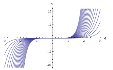
Figure 1: The potential (2.3) for various values of the parameter $\nu>1$ (and $\alpha>0$).

Here the main results obtained in Andrespapers1 ; Andrespapers2 ; Andrespapers3 are summarized. Consider the Einstein field equations minimally coupled to a scalar field

$$G_{\mu\nu}=\partial_{\mu}\phi\,\partial_{\nu}\phi-g_{\mu\nu}\left({\frac{1}{2}}g^{\rho\sigma}\partial_{\rho}\phi\,\partial_{\sigma}\phi+V(\phi)\right)$$ (3)

which through the Bianchi identity imply the Klein-Gordon equation,

$$\mathchoice{\vbox{\vbox{\hrule height=0.4pt\hbox{\vrule width=0.4pt,height=5.0pt\kern 5.0pt\vrule width=0.4pt}\hrule height=0.4pt}}}{\vbox{\vbox{\hrule height=0.4pt\hbox{\vrule width=0.4pt,height=5.0pt\kern 5.0pt\vrule width=0.4pt}\hrule height=0.4pt}}}{\vbox{\vbox{\hrule height=0.3pt\hbox{\vrule width=0.3pt,height=2.1pt\kern 2.1pt\vrule width=0.3pt}\hrule height=0.3pt}}}{\vbox{\vbox{\hrule height=0.3pt\hbox{\vrule width=0.3pt,height=1.5pt\kern 1.5pt\vrule width=0.3pt}\hrule height=0.3pt}}}\phi-V_{\phi}=0\,.$$ (4)

where $V_{\phi}\equiv dV/d\phi$. It was shown in Andrespapers1 that the most general potential compatible with the Carter-Debever-Plebański ansatz is

$$V(\psi)={\frac{\alpha}{\nu^{2}}}\left\{{\frac{\nu-1}{\nu+2}}\sinh[(1+\nu)\psi]+{\frac{\nu+1}{2-\nu}}\sinh[(\nu-1)\psi]-4{\frac{\nu^{2}-1}{4-\nu^{2}}}\sinh\psi\right\}\quad\hbox{with}\quad\psi\equiv\sqrt{\frac{2}{\nu^{2}-1}}\,\phi\,,$$ (5)

where $\alpha$, which has dimension $length^{-2}$, and $\nu>1$ are the parameters of the model. It is quite flat at the origin ($V(\psi)\simeq\alpha(\nu^{2}-1)\psi^{5}/30$) and is unbounded from below, see figure 1.

The equations (1-3) possess the following 4-dimensional, static and spherically symmetric solutions

$$\psi =\ln x\qquad,\qquad ds^{2}=\Omega(x)\left[-F(x)dt^{2}+{\eta^{2}\,dx^{2}\over F(x)}+d\theta^{2}+\sin^{2}\theta d\phi^{2}\right]$$ (6)

$$\hbox{with}\quad\Omega(x) ={\nu^{2}x^{\nu-1}\over\eta^{2}(1-x^{\nu})^{2}}\quad\hbox{and}\quad F(x)=\eta^{2}\,{x^{2-\nu}(1-x^{\nu})^{2}\over\nu^{2}}-\alpha\left[{1\over 4-\nu^{2}}+{x^{2}\over\nu^{2}}\left(1-{x^{-\nu}\over 2-\nu}-{x^{\nu}\over 2+\nu}\right)\right]\,,$$

where $\eta>0$ is the unique integration constant of the solution. This solution coincides with the Schwarzschild solution when $\nu=1$ (for details see Andrespapers2 ). The coordinate $x$ is dimensionless, related to the standard Droste radial coordinate $r$ as

$$r={\frac{\nu}{\eta}}\,{\frac{x^{\frac{\nu-1}{2}}}{|1-x^{\nu}|}}\,.$$ (7)

Spatial infinity is at $x=1$. The solutions have two branches: $0<x<1$, with the curvature singularity at $x=0$; and $x>1$, with the curvature singularity at $x=\infty$. Since $\Omega F\rightarrow 1$, $\eta^{2}\Omega/F(dx/dr)^{2}\rightarrow 1$ and $\Omega\approx r^{2}$ when $x\rightarrow 1$, the metric is asymptotically flat; and actually it is asymptotically Schwarzschild’s metric with PPN parameters $\gamma_{\mathrm{PPN}}=\beta_{\mathrm{PPN}}=1$.

The gravitational mass (read off from the asymptotic behaviour of the $g_{tt}=-(1-2m/r+\cdots)$ component of the metric) and the inertial mass of the solutions (as defined for example by the Komar integral or the Katz superpotential, see Andrespapers2 and KomarKatz ) are equal, and given by

$$m=\pm{\frac{\alpha+3\eta^{2}}{6\eta^{3}}}$$ (8)

with the upper sign for the branch $x<1$ and the lower for the branch $x>1$. The mass is positive for all $\alpha>-3\eta^{2}$ for the $x<1$ branch and for all $\alpha<-3\eta^{2}$ for the branch $x>1$.

The metric (6) represents a Schwarzschild-type black hole if the metric function $F(x)$ has one single zero, if it is positive at spatial infinity, and negative at the curvature singularity. These conditions are fulfilled

(a) when $\alpha>0$: for all $\eta$, if $\nu\in[1,2]$; and for $\eta^{2}-\frac{\alpha}{\nu-2}<0$ if $\nu>2$. In those cases the horizon $x_{+}$ is such that $0<x_{+}<1$ and the mass of the black hole is (2.6) with a plus sign;

(b) when $\alpha<0$: if $\eta^{2}+\frac{\alpha}{\nu+2}<0$. Then the horizon $x_{+}>1$ and the mass is (6) with a minus sign.

By definition, the horizon $x_{+}$ of the black hole is such that $F(x_{+})=0$ with $F$ given in (1.4) :

$$\eta^{2}=\alpha{\frac{\nu^{2}x_{+}^{\nu}-(\nu+2)x_{+}^{2}+(4-\nu^{2})x_{+}^{2+\nu}-(2-\nu)x_{+}^{2+2\nu}}{(4-\nu^{2})x_{+}^{2}(1-x_{+}^{\nu})^{2}}}\,.$$ (9)

The asymptotic behaviours of $\eta^{2}$ are :

$$\left\{\begin{aligned} {\eta^{2}\over\alpha}&\approx{1-x_{+}\over 3}\quad\hbox{for}\quad x_{+}\to 1\\ {\eta^{2}\over\alpha}&\approx-{1\over 2+\nu}(1-\nu x_{+}^{-\nu})\ \hbox{for}\ x_{+}\to\infty\end{aligned}\right.\quad,\quad\left\{\begin{aligned} {\eta^{2}\over\alpha}&\approx{\nu^{2}\,x_{+}^{\nu-2}\over 4-\nu^{2}}\to+\infty\quad\hbox{if}\quad\nu\in[1,2]\\ {\eta^{2}\over\alpha}&\approx{1\over\nu-2}\left(1-{\nu^{2}x_{+}^{\nu-2}\over\nu+2}\right)\quad\hbox{if}\quad\nu>2\end{aligned}\right.\quad\hbox{for}\quad x_{+}\to 0\,.$$ (10)

Besides these values of $x_{+}$, there is a further interesting value given by the condition $\frac{d(\eta)^{2}}{dx_{+}}=0$, whose numerator vanishes if

$$\frac{\nu-2}{\nu+2}=\frac{x_{+}^{\nu}-x_{+}^{2}}{x_{+}^{\nu+2}-1}.$$ (11)

Note that $x_{+}=1$ is a solution of (11), however it is not a critical point since $\left.\frac{d\eta^{2}}{dx_{+}}\right|_{x_{+}=1}=-\frac{\alpha}{3}$. Actually, since the LHS of (11) is such that $-\frac{1}{3}<\frac{\nu-2}{\nu+2}<1$ and the numerator as well as the denominator of the RHS of (11) are monotonically increasing or decreasing it follows that (11) can have at most one solution, which is $x_{+}=1$. Therefore, there are no critical points of the function (9) in the relevant interval and it is possible to parameterize the solution in terms of $x_{+}$ instead of $\eta$. The conditions (a,b) for the existence of an horizon can thus be replaced by (a’): $\alpha>0$, $x_{+}\in(0,1)$; (b’): $\alpha<0$, $x_{+}>1$.

The mass (8) of the black hole then becomes a function of $x_{+}$ or alternatively $r_{+}$ through (7) and (9). Then, it is possible to show that close to spacelike infinity we recover the Schwarzschild relation

$$\lim_{x_{+}\rightarrow 1}\frac{2m}{r_{+}}=1$$ (12)

and close to the singularities we have, using (10)

$$\left\{\begin{aligned} &\lim_{x_{+}\rightarrow 0}\,mr_{+}^{\nu-2}=(4-\nu^{2})^{(\nu-1)/2}(\sqrt{\alpha})^{1-\nu}/(2\nu)\qquad\hbox{for}\quad\alpha>0\quad\hbox{and}\quad\nu\in[1,2]\,,\\ &\lim_{x_{+}\rightarrow 0}\,m=(\nu+1)\sqrt{\nu-2}/(6\sqrt{\alpha})\qquad\hbox{for}\quad\alpha>0\quad\hbox{and}\quad\nu>2\,,\\ &\lim_{x_{+}\rightarrow\infty}\,m=\to(\nu-1)\sqrt{\nu+2}/(6\sqrt{-\alpha})\qquad\hbox{for}\quad\alpha<0\,.\end{aligned}\right.$$ (13)

We note that the mass can tend to a constant when the size of the black hole shrinks to zero.

III Linear instability

III.1 The Bronnikov et al. equations for linear radial perturbations

We summarize here the results obtained in Bronnikov1 ; Bronnikov2 . Consider the metric

$$ds^{2}=-e^{2[\gamma_{0}(x)+\delta\gamma(t,x)]}dt^{2}+e^{2[\alpha_{0}(x)+\delta\alpha(t,x)]}dx^{2}+e^{2\lambda_{0}(x)}(d\theta^{2}+\sin^{2}\theta\,d\phi^{2})$$ (14)

and scalar field $\phi=\phi_{0}(x)+\delta\phi(t,x)$. Expand the Einstein and Klein-Gordon equations (3) and (4) to linear order in the perturbations $\delta\gamma$, $\delta\alpha$ and $\delta\phi$. After rearrangement and proper use of the zeroth order, background, equations, they boil down to three independent equations. Two of them are constraints.

$$\delta\alpha ={\phi_{0}^{\prime}\over 2\lambda_{0}^{\prime}}\,\delta\phi$$ (15)

$$\delta\gamma^{\prime} ={1\over 2\lambda_{0}^{\prime 2}}\left[(\phi_{0}^{\prime}e^{-2\lambda_{0}}-\phi_{0}^{\prime}V-\lambda_{0}^{\prime}V_{\phi})e^{2\alpha_{0}}\delta\phi+\lambda_{0}^{\prime}\phi_{0}^{\prime}\,\delta\phi^{\prime}\right]$$

where a prime denotes derivation with respect to $x$ and where $V$ and $V_{\phi}$ are evaluated on the background solution $\phi_{0}$.

The third is an equation of propagation for $\delta\phi$, which, after setting

$$\delta\phi\equiv e^{\mathrm{i}Et}e^{-\lambda_{0}}u(x)\,,$$ (16)

can be put under the canonical form

$${\frac{d^{2}u}{d\rho^{2}}}+(E^{2}-V_{\mathrm{eff}})u=0$$ (17)

where $E$ is the “energy” of the mode, where $\rho$ is the “tortoise coordinate” such that

$$\rho^{\prime}\equiv{\frac{d\rho}{dx}}=e^{\alpha_{0}-\gamma_{0}}$$ (18)

and where the effective potential is given by

$$V_{\mathrm{eff}}={\frac{e^{2\gamma_{0}}}{\lambda_{0}^{\prime 2}}}\left[2\lambda_{0}^{\prime}\phi_{0}^{\prime}V_{\phi}-e_{0}^{-2\alpha_{0}}\lambda_{0}^{\prime 4}+\phi_{0}^{\prime 2}(V-e^{-2\lambda_{0}})+\lambda_{0}^{\prime 2}(e^{-2\lambda_{0}}-V+V_{\phi\phi})\right]\,.$$ (19)

III.2 The effective potential

The scalar field potential $V$ is given in (2.3) and the background solution is

$$\gamma_{0}=\ln\sqrt{\Omega F}\quad,\quad\alpha_{0}=\ln\eta\sqrt{\frac{\Omega}{F}}\quad,\quad\lambda_{0}=\ln\sqrt{\Omega},\quad,\quad\phi_{0}=\sqrt{\frac{\nu^{2}-1}{2}}\psi$$ (20)

with $\Omega$, $F$ and $\psi$ given in (2.4). Inserting (3.6) into (3.5) one finds

$$V_{\mathrm{eff}}=F{\frac{\mathrm{N}_{1}+x^{2}\mathrm{N_{2}}}{\mathrm{D}}}$$ (21)

and where the explicit expressions for $\mathrm{N}_{1}$, $\mathrm{N}_{2}$ and $\mathrm{D}$ are given in Appendix A.

Let us now look at the shape of the effective potential $V_{\mathrm{eff}}$. From its expression given in Appendix A we have that, near spatial infinity is simply

$$V_{\mathrm{eff}}=\left(\alpha-\eta^{2}\right)\left(x-1\right)^{3}+O(x-1)^{4}=O(\rho^{-3}).$$ (22)

Note that the condition (b’) for the existence of the horizon implies that whenever $x>1$ then $\alpha<0\Longrightarrow$ $V_{\mathrm{eff}}$ is negative close to spacelike infinity. The condition (a’), $\alpha>0$ and $x<1$ and the use of (10) shows that it is asymptotically negative if $\nu>3$; for $\alpha>0$ and $\nu\in[1,3]$ it can be positive close to spacelike infinity for small enough values of $x_{+}$.

Around the black hole horizon

$$d\rho=\frac{\eta dx}{F}=\frac{\eta dx}{(x-x_{+})F^{\prime}(x_{+})}+O(x-x_{+})^{-2},$$ (23)

therefore,

$$x>1\Longrightarrow\lim_{x\rightarrow x_{+}}\rho=\lim_{x\rightarrow x_{+}}\frac{\eta}{F^{\prime}(x_{+})}\ln\left|x-x_{+}\right|=+\infty,\qquad x<1\Longrightarrow\lim_{x\rightarrow x_{+}}\rho=\lim_{x\rightarrow x_{+}}\frac{\eta}{F^{\prime}(x_{+})}\ln\left|x-x_{+}\right|=-\infty$$ (24)

The effective potential (21) is overall multiplied by $F$, which implies that around the horizon

$$V_{\mathrm{eff}}(x=x_{+})\sim\exp\left(-\left|F^{\prime}(x_{+})\eta^{-1}\rho\right|\right)$$ (25)

From (22) and (25) it follows that the number of bound states with negative $E^{2}$ should be finite, as is the case with any potential tha fall-off faster than $\left|\rho\right|^{-2}$ in one dimension Reed:1979ne .

Near the horizon we have

$$V_{\mathrm{eff}}={\frac{dV_{\mathrm{eff}}}{dx}}\bigg{|}_{x_{+}}(x-x_{+})+\cdots\quad\hbox{with}\quad{\frac{dV_{\mathrm{eff}}}{dx}}\bigg{|}_{x_{+}}={\frac{dF}{dx}}{\frac{\mathrm{N_{1}}+x^{2}\mathrm{N_{2}}}{\mathrm{D}}}\bigg{|}_{x_{+}}$$ (26)

where $\mathrm{N_{1}}$, $\mathrm{N_{2}}$ and $D$ are given in Appendix A. The value of ${dV_{\mathrm{eff}}/dx}$ at $x=x_{+}$ is depicted in figure 2. For $\alpha>0$ it is negative unless the horizon size is small enough, all the more so as $\nu\rightarrow 1$. For $\alpha<0$ it is always negative for $\nu\in[1,3]$, and can be positive if $\nu>3$ and the horizon size is big enough all the more so as $\nu$ increases.

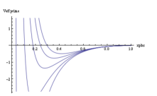
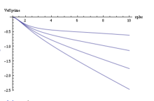
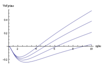
Figure 2: ${\frac{dV_{\mathrm{eff}}}{dx}}\big{|}_{x_{+}}$ as a function of the horizon location $x_{+}$ for various values of $\nu$. Left panel : $\alpha>0$ and increasing values of $\nu>1$ from right to left. Middle panel : $\alpha<0$ and $\nu\in[1,3]$. Right panel : $\alpha<0$ and increasing values of $\nu>3$ from right to left.

The effective potential can thus have three different shapes depending on the sign of $\alpha$, the value of the parameter $\nu$ and the location of the horizon $x_{+}$ : either is is negative everywhere, or it is a negative well edged by a barrier, at infinity if $\alpha>0$ or at the horizon if $\alpha<0$ ; or, if $\alpha>0$, it may be a negative well surrounded by two barriers, one near the horizon, the other at infinity. See figure 3 for two examples of such behaviours ; see figure 5 of Appendix D for a typical shape of a negative effective potential.

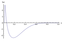
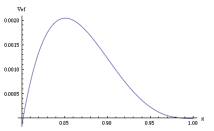
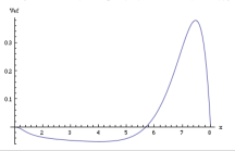
Figure 3: The effective potential $V_{\mathrm{eff}}$ as a function of the radial coordinate $x$ (the explicit expression of which is given in Appendix A). Left panel : for $\alpha>0$, $\nu=1.95$ and $x_{+}=0.02$, $V_{\mathrm{eff}}$ is a negative potential well surrounded by two barriers, one near the horizon $x_{+}$ and the other (zoomed on the medium panel) at spatial infinity. Right panel : for $\alpha<0$, $\nu=8$ and $x_{+}=8$.

III.3 The existence of bound states with negative $E^{2}$

For values of $\nu$ and $x_{+}$ such that the effective potential is everywhere negative then, as standard methods for solving the one dimensional Shrödinger equation show, the equation of motion (17) for the radial perturbations will possess bound states with negative $E^{2}$. Since, for a negative value of $E^{2}$, the mode $\delta\phi$ blows up in time, see (16), the black hole solution is then unstable.

For values of the parameters such that the effective potential is a negative well surrounded by positive barriers near the horizon and/or at infinity, then, in analogy with what happens in the case of a square potential well, bounded by a potential barrier, there will be no bound state and the radial perturbations will be stable, if the barrier is sufficiently high. As shown by Simon Simon1 ; Simon2 when $V_{\mathrm{eff}}$ is bounded and fall off faster than $\left|\rho\right|^{-2}$, a necessary (but not sufficient) condition for the absence of bound states of negative $E^{2}$ is

$$S\equiv\int_{-\infty}^{+\infty}V_{\mathrm{eff}}\,d\rho>0$$ (27)

It turns out that $S$ can be given in closed form. Its explicit expression is given in Appendix B. It is a function of $x_{+}$ and $\nu$ and its behavior is shown on figure 4. Its asymptotic behaviors are

$${S\over\sqrt{|\alpha|}} \approx-{\sqrt{3}\over 2}(|1-x_{+}|)^{3\over 2}\to 0_{-}\qquad\hbox{for}\ x_{+}\to 1_{\pm}$$ (28)

$$\alpha>0\ ,\ \nu\in[1,2]\leavevmode\nobreak\ :\quad{S\over\sqrt{\alpha}} \approx{\nu-1\over 4\nu}\sqrt{2-\nu\over 2+\nu}x_{+}^{-\nu/2}-{3\nu\over 2\sqrt{4-\nu^{2}}}x_{+}^{\nu/2-1}\to+\infty\quad\hbox{ for}\ x_{+}\to 0$$

$$\alpha>0,\nu>2\leavevmode\nobreak\ :\quad{S\over\sqrt{\alpha}} \approx{(\nu-1)\sqrt{\nu-2}\over 4(\nu+2)x_{+}}\to+\infty\quad\hbox{ for}\ x_{+}\to 0$$

$$\alpha<0\leavevmode\nobreak\ :\quad{S\over\sqrt{|\alpha|}} \approx-{7-\nu\over 4\sqrt{2+\nu}}x_{+}\left(1+{\nu-1\over(7-\nu)x_{+}}\right)\to\pm\infty\quad\hbox{for}\ x_{+}\to+\infty$$

When $\alpha>0$, $S$ is positive for all values of $\nu$ for small enough values of $x_{+}$. When $\alpha<0$, $S$ is positive for all values of $\nu>7$ for large enough values of $x_{+}$. Hence there is a possibility that there be no bound states in these cases and that the black hole solutions then be stable.

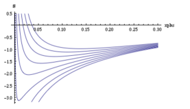
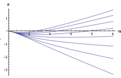
Figure 4: Simon’s integral $S$ as a function of the location of the horizon $x_{+}$ for various values of $\nu$, for $\alpha>0$ (left panel) and $\alpha<0$ (right panel). As can be seen it can be positive, for all values of $\nu$ if $x_{+}$ is small enough when $\alpha>0$, and for $\nu>7$ and $x_{+}$ big enough when $\alpha>0$.

Concentrating on cases when the Simon integral (27) is positive we hence integrated numerically the differential equation (17) using the standard “shooting” method (see e.g. Nath1 ). It consists in choosing the boundary value for $u(\rho)$ and its derivative in the potential barrier near the horizon in order to guarantee that the solution exponentially decreases as one approaches the horizon. A range of values for $E^{2}$ is then scanned (with $E^{2}$ negative but smaller than the depth of the well). If the corresponding mode functions $u(\rho,E^{2})$ all blow up exponentially for large $\rho$ to, say, $+\infty$, then the equation has no bound state. If, on the contrary, $u(\rho,E_{1}^{2})$ goes to $+\infty$ but $u(\rho,E_{2}^{2})$ goes to $-\infty$ then a bound state exists for a value $E_{n}^{2}\in[E_{1}^{2},E_{2}^{2}]$.

We did not explore the whole range of possibilities and limited ourselves to “reasonable” values of $\nu$ and $x_{+}$. Within these cases we were not able to find values for the parameters $\nu$ and $x_{+}$ which would not exhibit any bound state, see figure 6 in Appendix D for typical behaviors of the mode functions $u$.

Therefore the class of hairy black holes (2.4) are unstable, in that the spectrum of their spherically symmetric perturbations exhibits, at least generically, modes which grow exponentially in time.

However, as we shall now see, this instability can be marginal for small black holes.

IV A class of marginally stable small black holes

A first remark is, as was already established below eq. (25), is that the equation (17) for the radial perturbations possesses only a finite number of unstable bound states. Actually, our numerical exploration showed that for every value of the parameters there is only one bound state.

A second remark is that the eigenvalues of these bound states are bounded by a sharp Lieb-Thirring inequality Hundertmark:1998cz

$$\sum_{i}\sqrt{-E_{i}^{2}}\leq\frac{1}{2}\int_{V_{\mathrm{eff}}<0}\left|V_{\mathrm{eff}}\right|d\rho,$$ (29)

where the sum is for all $E_{i}^{2}<0$. Now, as is pointed out in Appendix A, $V_{\mathrm{eff}}$ is proportional to $\alpha$, therefore we can take $E^{2}=|\alpha|\bar{E}^{2}$ where $\bar{E}^{2}$ is a number, of order unity if the dimensionless parameters $\nu,$ $x_{+}$ and $\eta^{2}\alpha^{-1}$ are all taken of order unity (see examples of values of $\bar{E}^{2}$ in footnote 2). In that case the unstable mode

$$\delta\phi\propto e^{\mathrm{i}Et}=e^{+\sqrt{-\bar{E}^{2}}\,\sqrt{\alpha}\,t}$$ (30)

then grows on a time scale $t$ of the order of $1/\sqrt{\alpha}$. Since the characteristic time scale of gravitational effects is set by the mass $m$ of the black hole, the growth of the modes will be tamed if $\sqrt{\alpha}\,m$ is much less than 1. Returning to the relationship between the mass of the black hole and its horizon size given in (2.9) we therefore see that this condition is met if $\alpha>0$ and $\nu\in[1,2]$ in which case the mass and size of the black hole are related by

$$2\nu\sqrt{\alpha}\,m\approx(4-\nu^{2})^{(\nu-1)/2}(\sqrt{\alpha}\,r_{+})^{2-\nu}\ll 1\,.$$ (31)

Such black holes are therefore marginally stable, that is, “long-lived”.

V Conclusions

We studied in this paper the stability of the asymptotically flat black holes with minimally coupled scalar hair discovered in Andrespapers1 ; Andrespapers2 ; Andrespapers3 . We limited ourselves to the analysis of the radial “s-wave” perturbations of the metric and the scalar field, which can be presumed to be the least stable (since a stabilizing barrier in $l(l+1)/r^{2}$ appears in the effective potential of $l\neq 0$ modes). We found that, generically, some of these radial modes were spatially bounded but growing in time. Strictly speaking the black holes are therefore unstable. However, if their mass $m$ and size $r_{+}$ are small compared with the scale $1/\sqrt{\alpha}$ of the model the characteristic time for the instability to develop is long compared to the scale set by $m$.

A final remark is in order. Since the potential for the scalar field is unbounded from below, it is tempting to say that the instability could have been foreseen without any detailed analysis. However this would have been a hasty conclusion (as the well-known example of anti-de Sitter spacetime already teaches us AdSBH ). In fact, when a proper cosmological term is added to the potential, leaving it unbounded from below (see Andrespapers1 ; Andrespapers2 ; Andrespapers3 for its expression), so that the black hole is asymptotically anti-de Sitter, it is easy to see that the effective potential $V_{\mathrm{eff}}$ for the perturbations can be positive everywhere, so that the black hole is linearly stable against radial perturbations. We leave a thorough study of this promising case to further work.

While completing this work, an article that analyzes a similar situation and reaches conclusions which are in harmony with ours was published Kleihaus:2013tba .

Appendix A Explicit expression of the effective potential $V_{\mathrm{eff}}$

The effective potential (3.6) using (3.7) and (2.4) is :

$$V_{\mathrm{eff}}=F\,{\frac{\mathrm{N_{1}}+x^{2}\mathrm{N_{2}}}{\mathrm{D}}}$$ (32)

where $F$ is the metric function given in (2.4), where

$$\left\{\begin{aligned} {\rm D}&=4\beta\nu^{2}(4-\nu^{2})\,x^{2+\nu}\,[(\nu-1)+(\nu+1)x^{\nu}]^{2}\,,\\ {\rm N_{1}}&=c_{1}x^{2}+c_{2}x^{\nu}+c_{3}x^{2\nu}+c_{4}x^{3\nu}\quad,\quad{\rm N_{2}}=d_{1}x^{\nu}+d_{2}x^{2\nu}+d_{3}x^{3\nu}+d_{4}x^{4\nu}\end{aligned}\right.$$ (33)

and where the coefficients are given by

$$\left\{\begin{aligned} c_{1}&=-[1+\beta(2-\nu)](\nu+2)(\nu-1)^{4}\quad,\quad c_{2}=(3-\nu)(\nu-1)^{3}\nu^{2}\\ c_{3}&=6\nu^{2}(\nu^{2}-1)^{2}\quad,\quad c_{4}=-\nu^{2}(1+\nu)^{3}(3+\nu)\end{aligned}\right.$$ (34)

$$\left\{\begin{aligned} d_{1}&=(\nu-1)(\nu+2)[-4+5\nu-17\nu^{2}-\nu^{3}+\nu^{4}-4\beta(2-\nu)(2\nu^{3}+2\nu^{2}-\nu+1)]\\ d_{2}&=6(\nu^{2}-1)[2+11\nu^{2}-\nu^{4}+\beta(4-\nu^{2})(1+3\nu^{2})]\\ d_{3}&=(\nu+1)(\nu-2)[-4-5\nu-17\nu^{2}+\nu^{3}+\nu^{4}-4\beta(2+\nu)(-2\nu^{3}+2\nu^{2}+\nu+1)]\\ d_{4}&=(\nu-2)(\nu+1)^{4}[1+\beta(2+\nu)]\,.\end{aligned}\right.$$ (35)

where $\eta^{2}=\beta\alpha$. Finally $\beta$ can be writen in terms of $\nu$ and $x_{+}$ using the expresion given in (2.7). Hence $V_{\mathrm{eff}}/\alpha$ is a function of the radial coordinate $x$, the parameter $\nu$ and the location of the horizon $x_{+}$.

For $\nu=2$ (A.1-6) reduces to the effective potential studied in Appendix C. For $\nu=1$ it reduces to the “decoupling limit” effective potential studied in Appendix D.

Appendix B The Simon integral

Using (3.9) and the explicit expression for $V_{\mathrm{eff}}$ given Appendix A, we have that the Simon integral (3.13) reads

$$S=\pm\int_{x_{+}}^{1}V_{\mathrm{eff}}{\frac{d\rho}{dx}}dx=\pm\int_{x_{+}}^{1}{\frac{\eta\,(\mathrm{N_{1}}+x^{2}\mathrm{N_{2}})}{\mathrm{D}}}dx=\pm{\frac{\alpha}{\eta}}\,{\frac{\mathrm{S_{1}}}{\mathrm{S_{2}}}}\,,$$ (36)

where the plus sign holds for $\alpha>0$ and the minus sign for $\alpha<0$, where $\beta$ is given in terms of $x_{+}$ and $\nu$ in (2.7) and where

$${\rm S_{1}}= (\nu-1)(2-\nu)+2(\nu+1)(\nu+2)x_{+}-(\nu+2)(\nu+7)x_{+}^{2}$$ (37)

$$-2x_{+}^{\nu-1}[3\nu^{2}-2x_{+}(1+2\nu^{2})-x_{+}^{2}(\nu^{2}-4)-2x_{+}^{3}(7-\nu^{2})]$$

$$-x_{+}^{2\nu}[(\nu+1)(\nu+2)+2(2-\nu)(\nu-1)x_{+}+(7-\nu)(2-\nu)x_{+}^{2}]$$

and

$$\mathrm{S_{2}}=4(4-\nu^{2})x_{+}(1-x_{+}^{\nu})^{2}\,.$$ (38)

Appendix C The case $\nu=2$

When $\nu=2$ the general potential (2.3) and metric functions (2.4) have the following limits (with $\eta^{2}=\alpha\beta$) :

$$V ={\alpha\over 16}(-12\psi\cosh\psi+9\sinh\psi+\sinh 3\psi)\qquad\hbox{with}\qquad\psi=\sqrt{2\over 3}\,\phi$$ (39)

$$\Omega ={4x\over\alpha\beta(1-x^{2})^{2}}\qquad,\qquad F={\alpha\over 16}\left[(1-x^{2})(3-x^{2})+4\ln x+4\beta(1-x^{2})^{2}\right]\,.$$

The horizon of the black hole $x_{+}$ is such that $F(x_{+})=0$ and the parameter $\beta$ can thus be traded for its expression in terms of $x_{+}$ :

$$\beta=-{\frac{(x_{+}^{2}-1)(x_{+}^{2}-3)+4\ln x_{+}}{4(1-x_{+}^{2})^{2}}}\,.$$ (40)

The explicit expression of the effective potential $V_{\mathrm{eff}}$ (3.6) is not very illuminating : it is given by the limit of (A.1-5) for $\nu\to 2$. For $\alpha<0$ it is everywhere negative. For $\alpha>0$ its behaviour for $x_{+}$ small (e.g. $x_{+}=0.02$) is quite similar to that of figure 3. The Simon integral (3.13) is the limit of (B.1-3) for $\nu\to 2$ and reads

$${S\over\sqrt{\alpha}} ={(1-x_{+})\left[(1-x_{+}^{2})(1+12x_{+}+5x_{+}^{2})+12x_{+}(2+x_{+})\ln x_{+}\right]\over 8x_{+}(1+x_{+})\sqrt{-4\ln x_{+}-(1-x_{+}^{2})(3-x_{+}^{2})}}$$ (41)

$$\approx{1\over 8x_{+}\sqrt{-3-4\ln x_{+}}}+{5+12\ln x_{+}\over 4\sqrt{-3-4\ln x_{+}}}\qquad\hbox{for}\quad x_{+}\to 1\,.$$

$S$ has the same shape as in the generic case depicted in figure 4 (apart from the fact that it goes to $+\infty$ when $x_{+}\to 1$). It is positive for small enough $x_{+}$ (approximately, $x_{+}<0.01$).

The black holes are therefore unstable if $\alpha<0$. For $\alpha>0$ the effective potential may exhibit a positive barrier but, as in the generic case studied in the main text, we failed to find a range of $x_{+}$ for which there is no bound state. The black holes are therefore unstable.

Appendix D The “Decoupling Limit”

Consider the Klein-Gordon equation :

$$\mathchoice{\vbox{\vbox{\hrule height=0.4pt\hbox{\vrule width=0.4pt,height=5.0pt\kern 5.0pt\vrule width=0.4pt}\hrule height=0.4pt}}}{\vbox{\vbox{\hrule height=0.4pt\hbox{\vrule width=0.4pt,height=5.0pt\kern 5.0pt\vrule width=0.4pt}\hrule height=0.4pt}}}{\vbox{\vbox{\hrule height=0.3pt\hbox{\vrule width=0.3pt,height=2.1pt\kern 2.1pt\vrule width=0.3pt}\hrule height=0.3pt}}}{\vbox{\vbox{\hrule height=0.3pt\hbox{\vrule width=0.3pt,height=1.5pt\kern 1.5pt\vrule width=0.3pt}\hrule height=0.3pt}}}\psi-{\frac{dV}{d\psi}}=0\quad\hbox{with}\quad V={\frac{2\alpha}{3}}[\sinh\psi(\cosh\psi-4)+3\psi]\quad\hbox{so that}\quad{\frac{dV}{d\psi}}={\frac{4\alpha}{3}}(\cosh\psi-1)^{2}\,.$$ (42)

This is an odd potential which is very flat at $\psi=0$ ($V=\alpha\psi^{5}/15+\mathcal{O}(\psi^{6})$) and unbounded from below, of the type shown on figure 1.

On a Schwarzschild background,

$$ds^{2}=(1-2m/r)dt^{2}+{\frac{dr^{2}}{1-2m/r}}+r^{2}(d\theta^{2}+\sin^{2}\theta d\phi^{2}),$$ (43)

(where $m$ is a positive mass parameter), the field

$$\psi=\ln[1+1/(\eta r)],\qquad\hbox{with $\eta$ such that}\qquad 6\eta^{3}m+3\eta^{2}+\alpha=0,$$ (44)

solves the above Klein-Gordon equation (C.1). For $\psi$ to be bounded everywhere but at the singularity $r=0$, $\eta$ must be positive. Hence $\alpha<-3\eta^{2}$ must be negative.

The potential (D.1) and the Schwarzschlid metric (D.2) are the limit of the general potential and metric functions (2.3-4) when $\nu\to 1$, with $x\equiv 1+1/(\eta r)$.

At linear order the Schwarzschild metric is left unperturbed and, setting $\psi=\ln[1+1/(\eta r)]+\delta\psi(t,r,\theta,\phi)$, the perturbation $\delta\psi$ satisfies the following linear equation :

$$\mathchoice{\vbox{\vbox{\hrule height=0.4pt\hbox{\vrule width=0.4pt,height=5.0pt\kern 5.0pt\vrule width=0.4pt}\hrule height=0.4pt}}}{\vbox{\vbox{\hrule height=0.4pt\hbox{\vrule width=0.4pt,height=5.0pt\kern 5.0pt\vrule width=0.4pt}\hrule height=0.4pt}}}{\vbox{\vbox{\hrule height=0.3pt\hbox{\vrule width=0.3pt,height=2.1pt\kern 2.1pt\vrule width=0.3pt}\hrule height=0.3pt}}}{\vbox{\vbox{\hrule height=0.3pt\hbox{\vrule width=0.3pt,height=1.5pt\kern 1.5pt\vrule width=0.3pt}\hrule height=0.3pt}}}\delta\psi-{\frac{d^{2}V}{d\psi^{2}}}\Big{|}_{b}\,\delta\psi=0\,,\qquad\hbox{where}\qquad{\frac{d^{2}V}{d\psi^{2}}}\Big{|}_{b}=-{\frac{2(1+2\eta m)(1+2\eta r)}{r^{2}(1+\eta r)^{2}}}$$ (45)

is $d^{2}V/d\psi^{2}$ evaluated on the background solution (D.3), where we have traded $\alpha$ for $\alpha=-3\eta^{2}(1+2\eta m)$, and where      is the d’Alembertian on the Schwarzschild metric.

We decompose $\delta\psi$ in Fourier modes and spherical harmonics, and introduce the tortoise coordinate:

$$\delta\psi=e^{-\mathrm{i}Et}\,Y^{l}_{m}(\theta,\phi){\frac{u(r)}{r}}\qquad,\qquad\rho=r+2m\ln({r/2m-1})$$ (46)

so that the perturbed Klein-Gordon equation (D.4) reduces to

$${\frac{d^{2}u}{d\rho^{2}}}=(V_{\mathrm{eff}}-E^{2})u\qquad\hbox{with}\qquad V_{\mathrm{eff}}=\left(1-{\frac{2m}{r}}\right)\left({\frac{d^{2}V}{d\psi^{2}}}\Big{|}_{b}+{\frac{l(l+1)}{r^{2}}}+{\frac{2m}{r^{3}}}\right)$$ (47)

where $l$ is null or a positive integer and where $(d^{2}V/d\psi^{2})|_{b}$ is given in (D.4).

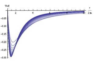
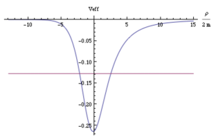
Figure 5: The “decoupling limit” effective potential $V_{\mathrm{eff}}$ when $l=0$. Left panel : for various values of the parameter $\eta$ and in fonction of $r$ ; rightpanel : for $\eta=0.5$ and in function of the tortoise coordinate $\rho$. Also is shown the (negative) value of $E^{2}$ corresponding to the bound state of figure 6.

When $l=0$, $V_{\mathrm{eff}}$ is negative for all $r>2m$ (for all positive $m$ and positive $\eta$), see figure 5. Bound states with negative $E^{2}$ therefore exist, which is confirmed by a numerical analysis of the solutions of (D.6), see figure 6.

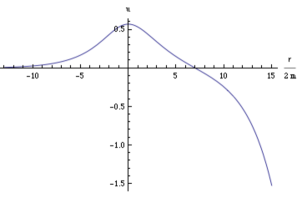
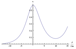
Figure 6: Solution of Eq. (D.6) for $\eta=0.5$. Left panel : for $E_{+}^{2}=-0.122$ ; right panel : for $E_{-}^{2}=-0.127$. A solution, bounded at the horizon and at infinity, exists for an eigenvalue $E_{1}^{2}$ such that $E_{-}^{2}<E_{1}^{2}<E_{+}^{2}<0$.

For a negative value of $E^{2}$, the mode $\delta\psi$ blows up in time. Therefore the solution (D.3) of the Klein-Gordon equation (D.1) is linearly unstable on the Schwarzschild background (D.2), if one imposes $m>0$ and that the background solution (D.3) diverges only at $r=0$, which requires $\eta>0$.