Fitting isochrones to open cluster photometric data

The metallicity is a critical parameter that affects the correct determination fundamental characteristics stellar cluster and has important implications in Galactic and Stellar evolution research. Fewer than $10\%$ of the 2174 currently catalog open clusters have their metallicity determined in the literature.
In this work we present a method for estimating the metallicity of open clusters via non-subjective isochrone fitting using the cross-entropy global optimization algorithm applied to UBV photometric data. The free parameters distance, reddening, age, and metallicity simultaneously determined by the fitting method. The fitting procedure uses weights for the observational data based on the estimation of membership likelihood for each star, which considers the observational magnitude limit, the density profile of stars as a function of radius from the center of the cluster, and the density of stars in multi-dimensional magnitude space.
We present results of [Fe/H] for nine well-studied open clusters based on 15 distinct UBV data sets. The [Fe/H] values obtained in the ten cases for which spectroscopic determinations were available in the literature agree, indicating that our method provides a good alternative to determining [Fe/H] by using an objective isochrone fitting. Our results show that the typical precision is about 0.1 dex.

1 Introduction

The accurate determination of the fundamental parameters of open clusters is essential in many fields of study in the Galactic and stellar evolution context. Important questions that depend on metallicity, which is usually measured by the [Fe/H] ratio, are the determination of chemical abundance gradients (see Lépine et al. (2011) and references therein), determination of the rotational speed of the spiral pattern, and the co-rotation radius (Dias & Lépine 2005), and in the stellar context the empirical determination of the initial mass function, among many other fields of study.

Typically, the determination of distances, ages, and reddening of open clusters via isochrone fitting requires either that the metallicity is estimated, or that an priory value is adopted. Therefore the metallicity is a required parameter for the precise determinating the open cluster’s fundamental characteristics. However, because of the complexity of the observations required and the sometimes very indirect methods needed to obtain this parameter, solar metallicity is often assumed.

[Fe/H] can be estimated from spectroscopic data, from low- to high-resolution, single or multi-object spectrographs as well as from photometric data. Each technique has advantages and disadvantages and limitations to the precision and accuracy that can be achieved. The discussion of methods and techniques that allow the determination of [Fe/H] is beyond the scope of this work, and we refer the reader the reviews of Gratton (2000) and Strobel (1991), among others. For the estimates of [Fe/H] obtained via photometric data we suggest the recent paper of Pöhnl & Paunzen (2010) and references therein.

In the last version of our open cluster catalog ( Dias et al. (2002) (DAML02)) we presented a compilation of [Fe/H] values obtained from the literature for 202 open clusters. This compilation is heterogeneous, since the metallicity determinations for a given cluster were made from different data sets and techniques as well as by different authors. Of all clusters with metallicity estimates, in the DAML02 catalog, we found that only 24% of the objects have estimates of their [Fe/H] ratio based on high-resolution spectra, 28% are based on low and medium-resolution spectra, and the rest are based on photometric data. Of those, 28% were estimated from isochrone fitting. Values range from about -0.8 dex to +0.5 dex and the errors range from 0.01 dex to 0.3 dex, depending on the method, number of stars and techniques used. Note that in general there are no estimates of the errors in [Fe/H] values obtained from isochrone fitting, and for the six existing cases, the uncertainty varies from 0.15 dex to 0.50 dex. Unfortunately, the subjectivity of the isochrone fitting makes it difficult to estimate a reliable error of the [Fe/H] ratio.

It is a well known fact that estimates of [Fe/H] obtained by high-resolution spectroscopy, which is the most reliable procedure, are obtained from only a few stars for any given open cluster. Due to the dispendious nature of executing spectroscopy, previous selection of the target stars is required, and thus the question of membership determination becomes important. Traditionally, the selection is made based on the color-magnitude diagram (see for example the paper of Carrera (2012)), choosing the red giant stars (usually the brightest stars of the cluster), or considering a study of membership probability based on proper motion and radial velocity data (e.g. Frinchaboy & Majewski (2008)). All these factors can seriously compromise the determination of the [Fe/H] ratio if they are not made properly.

Given that only $9\%$ of all the 2174 catalog open clusters have [Fe/H] estimated and that it is difficult to carry out detailed spectroscopic study for a large number of stars in a large sample of clusters, alternative and reliable methods are desirable.

In this work we focus on investigating the possibility of estimating the metallicity of open clusters via isochrone fitting using the cross-entropy global optimization algorithm (Monteiro et al. (2010), hereafter paper I), which allows simultaneous determination of distance, reddening, age and metallicity. In the second paper of this series (Dias et al. (2012), hereafter paper II) we presented a nonparametric procedure to assign membership likelihood based on photometric data of the stars, which in turn were used as weights in the CE isochrone fitting. To simplify the analysis in paper I and paper II we kept the metallicity constant at the value obtained from the literature which is used by most previous studies. In this paper we use the metallicity as a free parameter to be obtained from photometric UBV data and isochrone fitting using the CE method. In the next section we briefly review the CE method and data used. In Sect. 3 we present the estimated metallicity values obtained from the fitting method for each studied open cluster. In the last section we conclude by emphasizing important points, including potential applications and limitations of the work.

2 Method and data

In paper I we introduced a new technique to fit models to open cluster photometric data using a weighted likelihood criterion to define the goodness of fit and a global optimization algorithm known as cross-entropy (CE) to find the best-fitting isochrone.

Very schematically, the CE procedure provides a simple adaptive way of estimating the best-fit parameters. It involves an iterative procedure that follows the steps outlined below:

• random generation of the initial sample of fit parameters, respecting predefined criteria;

• selection of the best candidates based on calculated weighted likelihood values;

• generation of a random fit parameter sample derived from a new distribution based on the previous step;

• repeat until convergence or stopping criteria reached.

In paper II we introduced the nonparametric estimation of the likelihood to obtain a better estimate of the probability whether a given star is a member of the cluster. The weighting scheme uses observational data available in UBV filters for the open cluster and calculates the membership likelihood for each star considering observational magnitude limit, the density profile of stars as a function of radius from the center of the cluster, and the density of stars in multi-dimensional magnitude space. We refer to paper II for more details.

As in paper I and paper II, the tabulated isochrones used were taken from Girardi et al. (2000) and Marigo et al. (2008) and consisted of 400 files, one for each isochrone, which are specified by two parameters, namely, age and metallicity. To perform the isochrone fitting in this work we included the parameters distance and reddening to define the parameter space as follows:

1. Age: from $log(age)=$6.60 to $log(age)=$10.15; with steps of $log(age)=0.05$

2. distance: from 1 to 10000 parsecs;

3. ${\bf E(B-V)}$: from 0.0 to 3.0;

4. Metallicity: from 0.0001 to 0.03 dex with steps of $Z=0.05$ dex

Applied our fitting procedure to the UBV data from the literature for the same open clusters analysed in paper I and paper II. Apart from adopting metallicity as a free parameter, in this work all procedures are identical to those in paper II.

To determine the parameter errors through Monte Carlo techniques we performed the fit for each data set ten times, each time resampling from the original data set, with replacement, to perform a bootstrap procedure. In each bootstrap iteration new isochrone points from the adopted initial mass function were also generated as described in paper I, paper II, and in Monteiro & Dias (2011). The final uncertainties in each parameter were then obtained by calculating the standard deviation of the ten runs.

In previous papers of this series we have shown that the CE method was robust, and the results obtained for the ten open clusters investigated agree well with previous studies found in the literature, considering UBV data (paper I), BVRI data (Monteiro & Dias 2011) and also near-infrared (JH$K_{s}$) data obtained from the 2MASS catalog (paper II). The method presents several advantages over visual fits, especially since it removes most of the related subjectivity both in the fit and in the weights of the stars in the color-magnitude diagram (hereafter CMD), while also allowing us to determine the parameter errors in a formal procedure. The main limitation is that we do not yet account for missing data. In other words, for a star to be considered, it has to have been observed in all used filters. This problem is being investigated and will be implemented for future versions of the algorithm.

3 Results and discussion

As in papers, Table 1 presents the tuning parameters used in the fitting procedure, where list the equatorial coordinates ($\alpha,\delta$) and the radius, which were obtained from the DAML02 catalog and $x_{c}$ and $y_{c}$ are the estimated center coordinates of the cluster in the CCD, based on the determined 2D density distribution of stars. The parameter $V_{cut}$ is the adopted cut-off in V magnitude based on the completeness analysis in that band, and $\mathbf{F}_{bin}$ is the binary fraction. The binary fraction was changed in some cases to 50% from the adopted 99% where it clearly improved the final fit. The paramenter $3\sigma_{phot}$ the photometric error and $P_{cut}$ the adopted cut-off in weight values. The WEBDA catalog (Mermilliod 1995) reference codes are the same as those given in papers.

Figure 1: Comparison of our fit results with those of paper II for E(B-V), distance and age (upper left, right and lower left respectively). Comparison of final estimated metallicity values with those from the literature are given in the lower right plot. The error bars are those presented in Table 2 for the fits as explained in the text. The lines of 45^∘ are the loci of equal values. The [Fe/H] values obtained are compared with those from the DAML02 catalog. The filled symbols indicate [Fe/H] from high-resolution spectra.

We present the comparison of the results obtained in this work with those obtained in paper II in the first three plots of Fig. 1 for the nine open clusters. The last plot shows the metallicity values we determined in this work compared with literature values from the DAML02 catalog, which were obtained from spectroscopy.

The average and standard deviation of the differences of our results to those of paper II are

E(B-V)= $0.03\pm 0.05$ $mag$;

Distance= $-63\pm 262$ $pc$;

Log(age)= $-0.01\pm 0.18$ $yr$.

One can see from the comparison of the results that distance, E(B-V) and age values obtained in paper II were recovered in this work, within the uncertainties of the method.

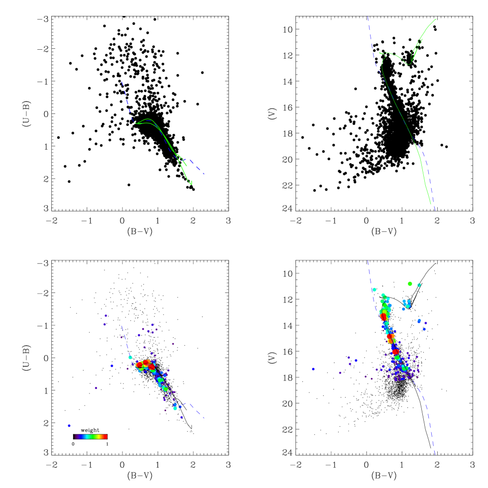
Figure 4: Results for the open cluster NGC 2477. Upper graphs show available UBV data and lower ones the weighted data (with symbol size and color ranging proportional to membership likelihood), the fitted isochrone (solid line) and the ZAMS (dashed line).

The fit results obtained by the method applied to the UBV data for each cluster can be seen in Figs. 4 through 18 in Appendix A. The figures present the CMDs with the original data followed by the same plots, with the symbol sizes reflecting the weights used as obtained from the procedure introduced in paper II. The fitted isochrone and zero age main sequence are also plotted. In Tables 2 and 3 we present the final fit values for each cluster studied with the metallicity as a free parameter in the fitting procedure. To facilitate the comparison, the parameter values obtained in paper II are also provided, including the metallicity adopted from the literature. The final value of this parameter was transformed to [Fe/H], adopting the same approximation as considered in the Padova database of stellar evolutionary tracks and isochrones: $[Fe/H]=logZ/Z\odot$ with $Z\odot=0.019$. The errors were obtained by the usual propagation formula.

In Table 3 our results for [Fe/H] are compared with those from the literature where we also provide information on the method used in the given reference to determine it. In comparing our results with those in the literature that used spectroscopy to obtain [Fe/H], we find that the average difference is 0.08 dex with a standard deviation of 0.07 dex, with no significant difference between regular or high-resolution spectroscopy (HRS).

The [Fe/H] values we determine agree with those obtained from the literature considering the previous comparison. The mean of the differences shows that there is no significant systematic trend, and the low value of the mean square difference indicates that both sets of measurements agree. Considering that the values obtained by HRS are the most reliable, the agreement of our values with those in the literature indicates that our method provides adequate results for [Fe/H] by isochrone fitting. It would be interesting to fit a large number of clusters to confirm this as well as to allow investigation of possible biases.

Below we comment on some individual open cluster results.

3.1 NGC~2477

The metallicity determined from our fitting procedure for the cluster NGC 2477 is just outside of the $1\sigma$ agreement region, which can be seen in Fig. 1, considering [Fe/H] values from DAML02 catalog. In DAML02 the value from Bragaglia et al. (2008) was adopted estimated on the basis of six stars from HRS. Comparing their results with those from Friel et al. (2002), the authors consider, the possibility that their metallicities could be generally bigher by about 0.2 dex. The values in Table 3 indicate the possibility of lower metallicity for NGC~2477. Considering the original photometric data (Kassis et al. 1997) (REF 152), our results agree with those obtained by the authors, who used $[Fe/H]=-0.05\pm 0.11$ dex from moderate resolution spectroscopy of seven cluster giants determined by Friel & Janes (1993). Another interesting point is that our values agree with those of Jeffery et al. (2011). In that study the authors employed a new Bayesian statistical technique that performs an objective, simultaneous model fit of the cluster and stellar parameters with the photometry. The authors used BVI photometric data, obtaining E(B-V) = 0.198, distance of 1411 pc and logt of 9.04, and $[Fe/H]=-0.34\pm 0.07$ dex. The [Fe/H] value estimated by our fit agrees within the uncertainties with the values published previously by Friel & Janes (1993) and Jeffery et al. (2011). Possibly a more complete UBVRI data set togheter with the CE algorithm could confirm the value of [Fe/H] for the object.

3.2 NGC~2355

The open cluster NGC~2355 also shows significant differences in the estimated metallicity with the data set from Ann et al. (1999) (REF. 217) when compared with literature values obtained from spectroscopy. Despite the obtained errors in [Fe/H], the discrepancy in this case seems to be due to a systematic difference in the photometry of the two sets. The data from Ann et al. (1999) are systematically redder than the one from Kaluzny & Mazur (1991c) (REF. 44). To show this difference, we took the two data sets and calculated color-index averages for specific V-magnitude bins. The stars used in each bin from each data set are the same, to avoid biases and selection effects. We then plotted the values in the CMD. For the locus where the giants are, we defined a box such that $10<V<14$ and $(B-V)>0.8$ to obtain the color-index average. For the rest of the data we used a V-magnitude bin of 1. The result is shown in Fig.2. This example is useful to illustrate that the quality of the [Fe/H] estimate obtained by fitting is directly linked to the quality of the data, even considering the improved statistical fitting procedures.

Figure 2: Comparison of average color-index values for the two data sets used for the open cluster NGC~2355. The differences in data sets explain the differences in the parameters obtained with the cross-entropy method, specially distance and metallicity.

3.3 NGC~7044

Our result for the open cluster NGC~7044 also shows a significant difference from the result of Warren & Cole (2009) obtained using spectroscopy. Unlike the case for NGC~2355 mentioned before, here we did not have a second data set with UBV photometry to compare distinct fit results. However, we were able to compare the observational data by using the B and V values obtained by Kaluzny (1989) and Sagar & Griffiths (1998). To perform the comparison, we followed the same strategy as before where we calculated color-index averages for specific V-magnitude bins in the CMD considering the same stars. For the giant locus in the CMD of NGC~7044 we defined a box such that $14<V<17$ and $(B-V)>1.5$ to obtain the color-index average. For the rest of the data we used a V-magnitude bin of 1. The result of the comparison is shown in Fig. 3, where it is clear that there is a considerable difference in the photometry. Even though we were not able to perform fits to the data from Kaluzny (1989) and Sagar & Griffiths (1998) since they only observed B and V filters, it is likely that the photometric differences shown are an important factor in accounting for the discrepancy in metallicity that we found.

Figure 3: Comparison of mean color-index values for the data set used in the fit of the open cluster NGC~7044 and the data sets of Sagar & Griffiths (1998) (REF 162) and Kaluzny (1989) (REF 13). The differences in the data sets are a possible cause of the discrepancy between the value obtained for the metallicity by our fit and the one of Warren & Cole (Warren & Cole (2009)), which was obtained with spectroscopy.

Table 1: Cross-entropy fit parameters. The first five columns (after the cluster identification) give the central coordinates and radius from the DAML02 catalog, followed by the X,Y central position used considering UBV data from the literature. The parameter $V_{cut}$ is the adopted cut-off in magnitude in V, $\mathbf{F}_{bin}$ is the number of stars considered as binary, $3\sigma_{phot}$ the photometric error, and $P_{cut}$ the adopted normalized likelihood cut-off. The reference codes given in last column are the same as used by WEBDA and were also used in paper I.

Cluster	$\alpha$	$\delta$	RADIUS	$x_{c}$	$y_{c}$	$V_{cut}$	$\mathbf{F}_{bin}$	$3\sigma_{phot}$	$P_{cut}$	REF
	J2000.0	J2000.0	arcmin	pix	pix	(mag)	(%)	(%)	(%)
NGC~2477	07 52 10	-38 31 48	15	-40.97	-160.82	18.25	50	1.0	5.0	152
NGC~7044	21 13 09	+42 29 42	06	13.27	31.35		99	1.5	10	62
NGC~2266	06 43 19	+26 58 12	05	0.05	7.94		99	1.0	5.0	41
Berkeley 32	06 58 06	+06 26 00	06	734.22	662.30		99	1.0		40
NGC~2682	08 51 18	+11 48 00	25	-0.01	-0.43		99	1.5		335
				-0.22	-0.83		50	1.5		31
				0.00	-1.64		50	1.5	5.0	54
NGC~2506	08 00 01	-10 46 12	12	-9.58	-16.10		99	1.0	30	284
				-10.85	8.30	17.75	99	1.5	5.0	163
NGC~2355	07 16 59	+13 45 00	07	33.30	12.38		99	1.5		217
				17.97	3.40		99	1.5	5.0	44
Melotte~105	11 19 42	-63 29 00	05	-39.31	-35.96		99	1.5	5.0	289
				11.18	-34.34	16.75	99	1.5		32
Trumpler~1	01 35 42	+61 17 00	03	1.54	-2.04	17.75	99	1.5	5.0	320
				-19.05	0.68	17.75	99	1.0		86

References:

152 = Kassis et al. (1997)

62 = Aparicio et al. (1993)

41 = Kaluzny & Mazur (1991b)

40 = Kaluzny & Mazur (1991a)

335 = Henden (2003)

31 = Gilliland et al. (1991)

54 = Montgomery et al. (1993) (adopted logt = 9.6)

284 = Kim et al. (2001) (adopted mean values: see Table 5 of the paper)

163 = Marconi et al. (1997)

217 = Ann et al. (1999)

44 = Kaluzny & Mazur (1991c)

289 = Sagar et al. (2001)

32 = Kjeldsen & Frandsen (1991)

320 = Yadav & Sagar (2002)

86 = Phelps & Janes (1994)

Table 2: Parameters obtained for the investigated clusters with the cross-entropy method considering the metallicity as a free parameter. In the first three columns (after the cluster identification) we reproduce the results published in paper II to facilitate comparison. In the following three columns the results for $E(B-V)$ the extinction, distance to the cluster and $\log(Age)$ the logarithm of the age (in years) obtained in this work are presented. The reference codes given in last column are the same as given in Table 1. See the text for error estimate details.

	paper II			This work
Cluster	$E(B-V)$	Distance	Log(Age)	$E(B-V)$	Distance	Log(Age)	REF
	(mag)	(pc)	(yr)	(mag)	(pc)	(yr)
NGC~2477	0.29 $\pm$ 0.02	1565 $\pm$ 103	8.83 $\pm$ 0.05	0.31 $\pm$ 0.03	1341 $\pm$ 106	8.85 $\pm$ 0.09	152
NGC~7044	0.53 $\pm$ 0.01	3323 $\pm$ 116	9.32 $\pm$ 0.16	0.66 $\pm$ 0.04	3326 $\pm$ 176	9.10 $\pm$ 0.05	62
NGC~2266	0.15 $\pm$ 0.01	3285 $\pm$ 289	8.82 $\pm$ 0.08	0.20 $\pm$ 0.02	3000 $\pm$ 197	8.80 $\pm$ 0.06	41
Berkeley 32	0.14 $\pm$ 0.02	3271 $\pm$ 83	9.62 $\pm$ 0.13	0.15 $\pm$ 0.03	3078 $\pm$ 88	9.70 $\pm$ 0.14	40
NGC~2682	0.03 $\pm$ 0.01	765 $\pm$ 52	9.48 $\pm$ 0.23	0.09 $\pm$ 0.03	818 $\pm$ 95	9.30 $\pm$ 0.46	335
	0.10 $\pm$ 0.02	802 $\pm$ 30	9.05 $\pm$ 0.28	0.06 $\pm$ 0.06	803 $\pm$ 78	9.40 $\pm$ 0.49	31
	0.04 $\pm$ 0.01	792 $\pm$ 20	9.45 $\pm$ 0.08	0.03 $\pm$ 0.01	808 $\pm$ 90	9.45 $\pm$ 0.10	54
NGC~2506	0.03 $\pm$ 0.04	3349 $\pm$ 795	9.20 $\pm$ 0.16	0.03 $\pm$ 0.01	2970 $\pm$ 563	9.30 $\pm$ 0.19	284
	0.05 $\pm$ 0.01	3533 $\pm$ 144	9.10 $\pm$ 0.10	0.10 $\pm$ 0.03	3750 $\pm$ 640	9.00 $\pm$ 0.17	163
NGC~2355	0.26 $\pm$ 0.01	2083 $\pm$ 243	8.82 $\pm$ 0.10	0.32 $\pm$ 0.09	1503 $\pm$ 504	8.95 $\pm$ 0.22	217
	0.18 $\pm$ 0.02	2213 $\pm$ 238	8.85 $\pm$ 0.07	0.22 $\pm$ 0.05	1949 $\pm$ 338	8.90 $\pm$ 0.10	44
Melotte~105	0.48 $\pm$ 0.02	1701 $\pm$ 329	8.48 $\pm$ 0.18	0.53 $\pm$ 0.05	1715 $\pm$ 193	8.55 $\pm$ 0.11	289
	0.57 $\pm$ 0.06	1910 $\pm$ 285	8.48 $\pm$ 0.18	0.50 $\pm$ 0.02	1873 $\pm$ 226	8.40 $\pm$ 0.08	32
Trumpler~1	0.62 $\pm$ 0.04	2145 $\pm$ 78	7.75 $\pm$ 0.25	0.68 $\pm$ 0.06	2469 $\pm$ 381	7.30 $\pm$ 0.35	320
	0.62 $\pm$ 0.04	2339 $\pm$ 146	7.00 $\pm$ 0.18	0.61 $\pm$ 0.06	2722 $\pm$ 402	7.05 $\pm$ 0.19	86

Table 3: Parameter metallicity obtained for the clusters investigated with the cross-entropy method. In the first column we list the cluster identification, the second column shows the metallicities obtained from the literature for the investigated clusters, and the third column presents the literature codes. In the column TEC we give the technique of data acquisition used for [Fe/H] determination, named SPEC for spectroscopy and PHOT for photometry. The last two columns present the metallicity values obtained in this work and the reference code for the data used from the WEBDA catalog. See the text for error estimates details.

				This work
Cluster	[Fe/H]	literature code	TEC code	[Fe/H]	REF
NGC~2477	0.07 $\pm$ 0.03	R01	SPEC	-0.10 $\pm$ 0.12	152
	-0.03$\pm$ 0.07	R03	PHOT
	-0.008	R07	PHOT
	-0.13$\pm$ 0.18	R08	PHOT
	-0.34$\pm$ 0.07	R09	PHOT
	-0.05$\pm$ 0.11	R10	SPEC
	0.04$\pm$ 0.01	R11	SPEC
	0.019$\pm$ 0.115	R12	SPEC
	0.05	R13	PHOT
	0.07$\pm$ 0.03	R28	SPEC
NGC~7044	-0.16 $\pm$ 0.09	R14	SPEC	0.04 $\pm$ 0.10	62
	0.0 $\pm$ 0.2	R27	PHOT
	0.01	R13	PHOT
	0.01$\pm$ 0.10	R03	PHOT
NGC~2266	-0.26 $\pm$ 0.02	R02	PHOT	-0.32 $\pm$ 0.14	41
	-0.26 $\pm$ 0.2	R03	PHOT
	-0.38 $\pm$ 0.06	R15	SPEC
Berkeley 32	-0.29 $\pm$ 0.04	R01	SPEC	-0.38 $\pm$ 0.11	40
	-0.42 $\pm$ 0.09	R03	PHOT
	-0.37 $\pm$ 0.05	R16	PHOT
	-0.3 $\pm$ 0.02	R17	SPEC
	-0.37 $\pm$ 0.04	R18	PHOT
	-0.55	R13	PHOT
NGC~2682	0.03 $\pm$ 0.02	R04	SPEC	0.0 $\pm$ 0.18	335
	-0.029	R07	PHOT	0.04 $\pm$ 0.10	31
	-0.04$\pm$ 0.03	R03	PHOT	0.04 $\pm$ 0.10	54
	-0.05 $\pm$ 0.03	R19	PHOT
	-0.06 $\pm$ 0.07	R20	PHOT
	-0.05 $\pm$ 0.04	R18	PHOT
	-0.01 $\pm$ 0.11	R21	PHOT
	0.000 $\pm$ 0.092	R12	PHOT
	-0.11	R13	PHOT
	-0.09 $\pm$ 0.07	R10	SPEC
	-0.01 $\pm$ 0.05	R06	SPEC
NGC~2506	-0.2 $\pm$ 0.02	R05	SPEC	-0.13 $\pm$ 0.16	284
	-0.51 $\pm$ 0.1	R03	PHOT	-0.13 $\pm$ 0.16	163
	-0.19 $\pm$ 0.06	R22	SPEC
	-0.24 $\pm$ 0.05	R23	SPEC
	-0.44 $\pm$ 0.06	R24	SPEC
	-0.58 $\pm$ 0.14	R08	PHOT
	-0.52 $\pm$ 0.07	R10	SPEC
	-0.57	R25	PHOT
	-0.48 $\pm$ 0.08	R21	PHOT
	-0.58	R13	PHOT
	-0.368 $\pm$0.108	R12	PHOT
NGC~2355	-0.08 $\pm$ 0.08	R06	SPEC	-0.32 $\pm$ 0.14	217
	0.02$\pm$0.2	R03	PHOT	-0.23 $\pm$ 0.24	44
	0.13	R26	PHOT
Melotte~105	0.0	R13	PHOT	-0.05 $\pm$ 0.15	289
	0.0 $\pm$ 0.1	R03	PHOT	0.00 $\pm$ 0.21	32
Trumpler~1	-0.71	R13	PHOT	0.10 $\pm$ 0.13	320
	-0.71 $\pm$ 0.1	R03	PHOT	0.15 $\pm$ 0.10	86

4 Conclusions

The observational complexity and difficulty in carrying out detailed high-resolution spectroscopy of a large number of stars for a large number of clusters raises the question of alternative methods for estimating their metallicity reliably . The observational complexities account for the very small number of clusters, fewer than 10% in DAML02 catalog, for which good-quality metallicities exist. As commented by Paunzen et al. (2010), the metallicity parameter is set as solar or ignored in most papers that perform some sort of isochrone fitting in CMDs when this parameter is not available from other sources, possibly introducing an unknown bias in the distance, age and reddening estimated.

Our method, based on the Cross-Entropy optimization algorithm, using UBV photometric data weighted with a membership-likelihood estimation, allows for the simultaneous determination of the parameters distance, reddening, age and, as shown in this work, metallicity. The main advantage, as discussed in detail in the previous works of the series, is the automation and removal of subjectivity in the fitting process. All fitting parameters are clearly defined and the fitting quality is quantifiable through the likelihood, which can be objectively compared with any proposed alternative.

In this work we present [Fe/H] estimates obtained with the CE method for nine well-studied open clusters based on 15 distinct UBV data sets. The comparison with [Fe/H] obtained by spectroscopy indicates that our results are adequate for obtaining low-telescope-cost metallicity estimates since most values are consistent withing the $1\sigma$ uncertainty. Our bootstrap-estimated errors for [Fe/H] values also show the good agreement between our results and literature [Fe/H] values obtained from photometric as well as spectroscopic data.

It is important to point out that the accuracy and precision as well as the overall quality of the photometric data are decisive for the quality of the final estimated metallicity.

Generally, visual isochrone fits can provide estimates of the metallicity, but typically do not provide estimates of the error (in some works the error estimates are given as in Vázquez et al. (2010), although obtained by visual fit). Our method provides a robust [Fe/H] with consistent error estimates. Our results show a typical internal precision of about 0.1 dex.

Finally, we emphasize the conclusion of paper I, but now with the extra parameter metallicity included, that our method is reliable and robust in determining the distance, age, reddening, and metallicity by isochrone fits. It is a powerful tool that in the near future can be used with already existing data and especially in upcoming modern large surveys, such as GAIA, VISTA, and Pan-STARRS to produce homogeneous large samples of determined fundamental parameters of open clusters.

Appendix A Fit results

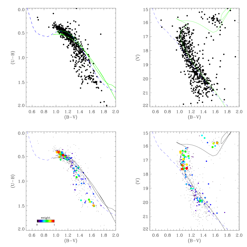
Figure 5: Same as Fig. 4 for NGC 7044.

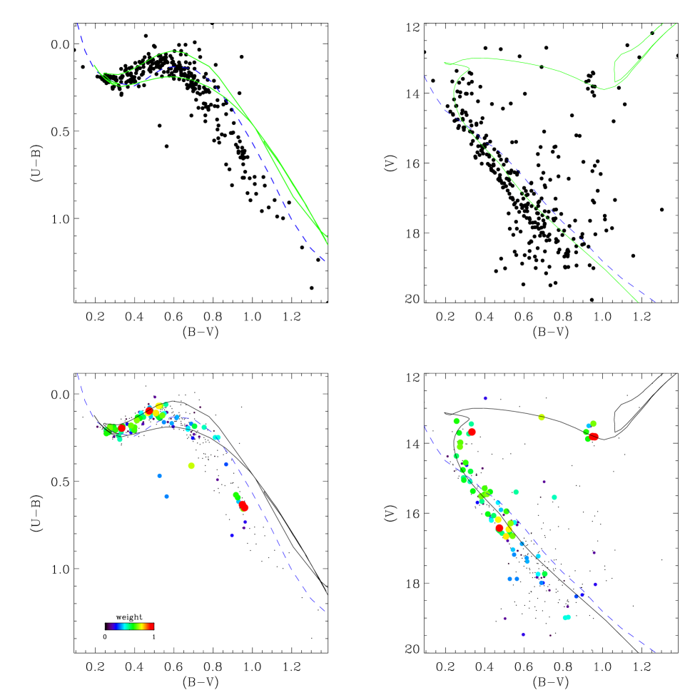
Figure 6: Same as Fig. 4 for NGC 2266.

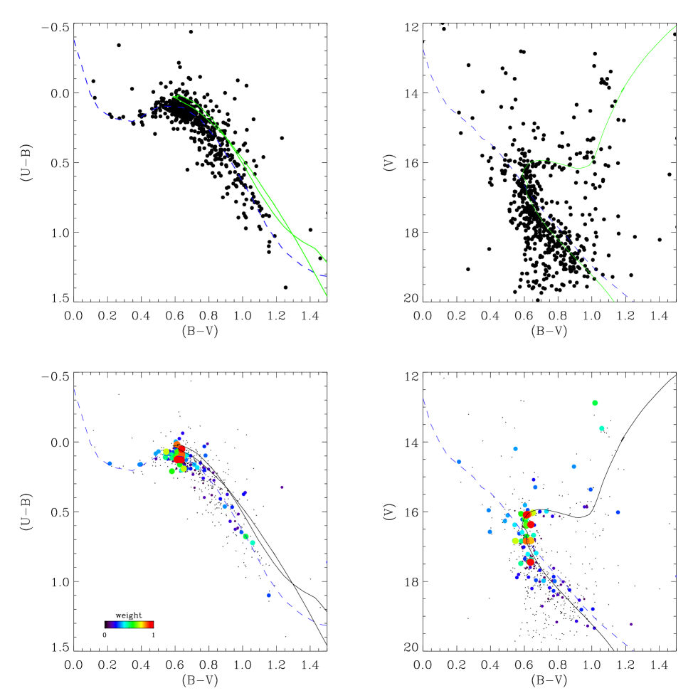
Figure 7: Same as Fig. 4 for Berkeley 32.

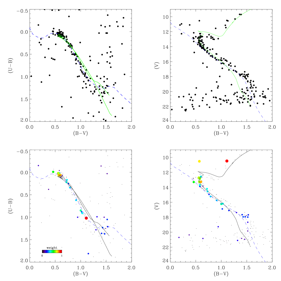
Figure 8: Same as Fig. 4 for NGC 2682 (Ref. 31).

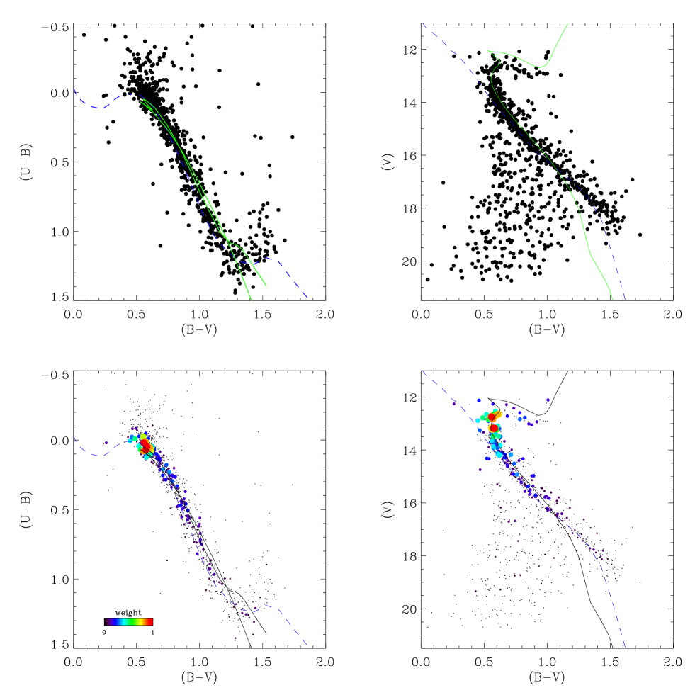
Figure 9: Same as Fig. 4 for NGC 2682 (Ref. 54).

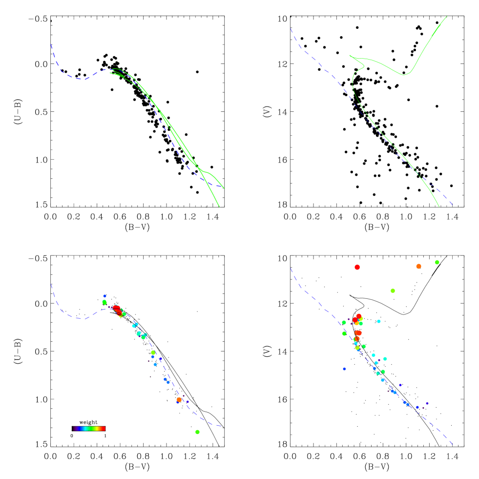
Figure 10: Same as Fig. 4 for NGC 2682 (Ref. 335).

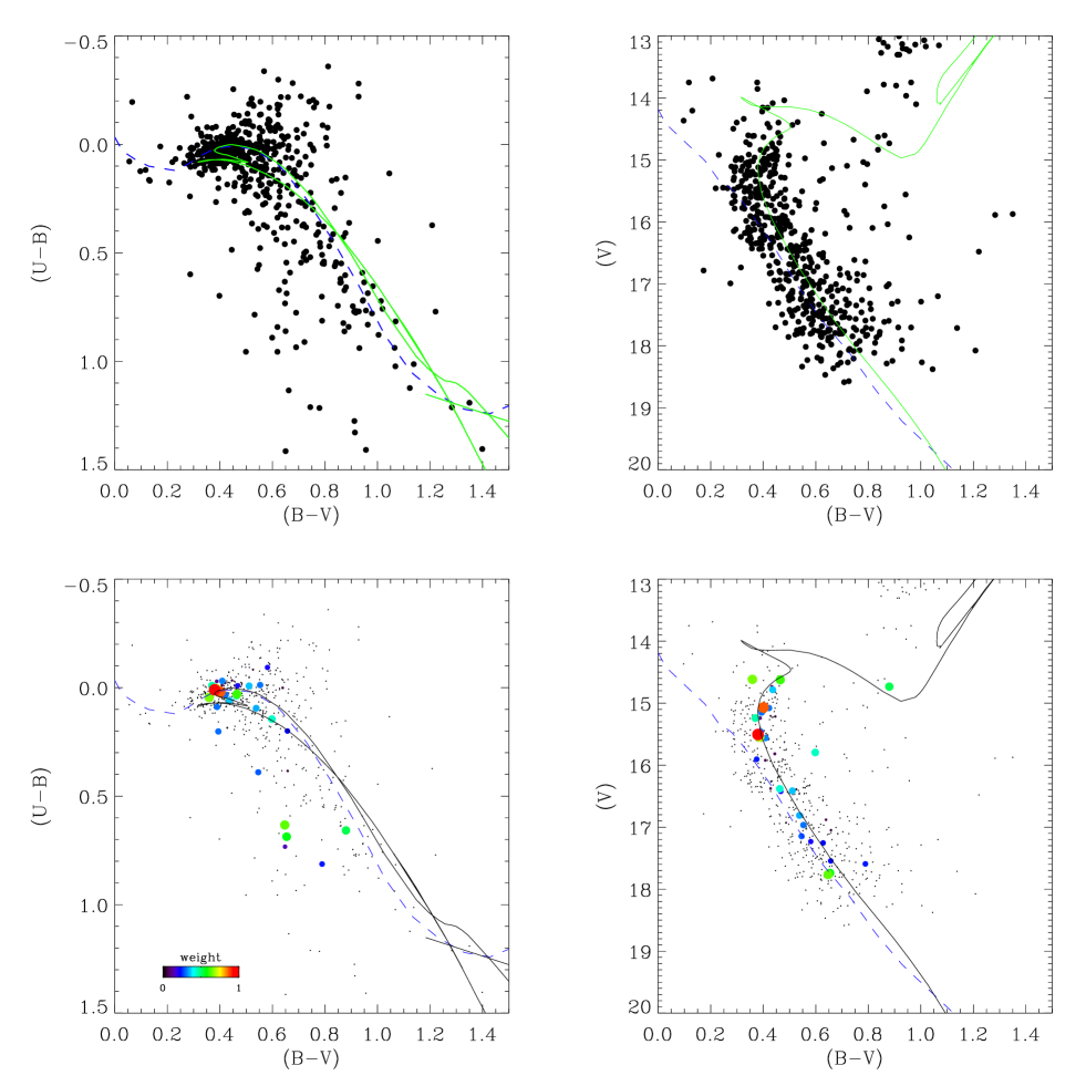
Figure 11: Same as Fig. 4 for NGC 2506 (Ref. 284).

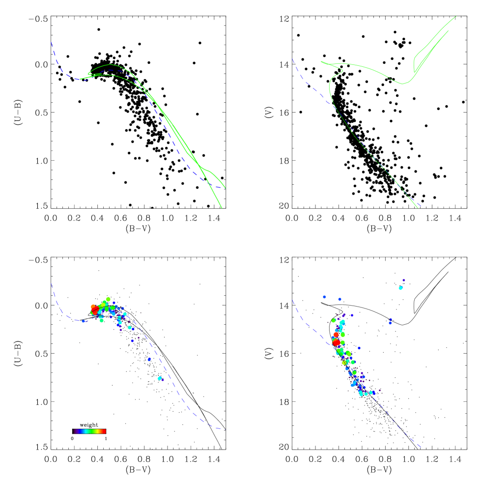
Figure 12: Same as Fig. 4 for NGC 2506 (Ref. 163).

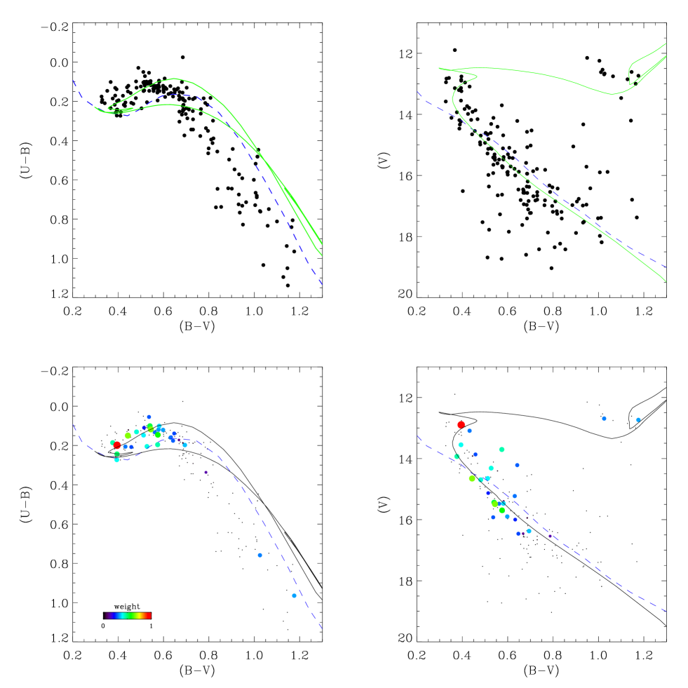
Figure 13: Same as Fig. 4 for NGC 2355 (Ref. 44).

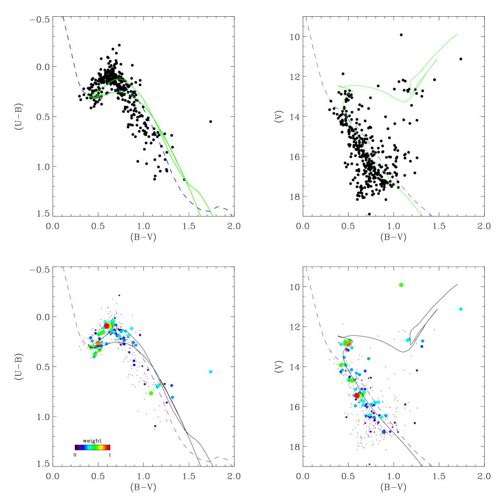
Figure 14: Same as Fig. 4 for NGC 2355 (Ref. 217).

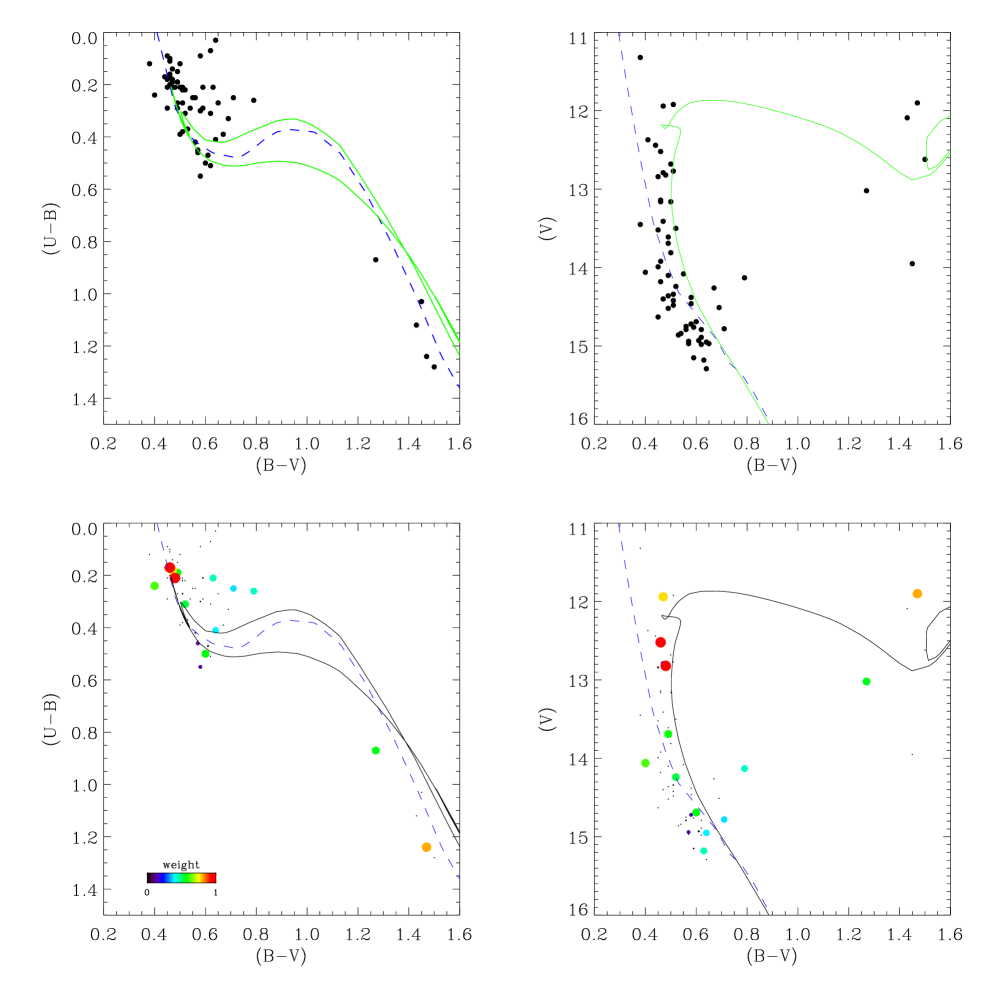
Figure 15: Same as Fig. 4 for Melotte 105 (Ref. 289).

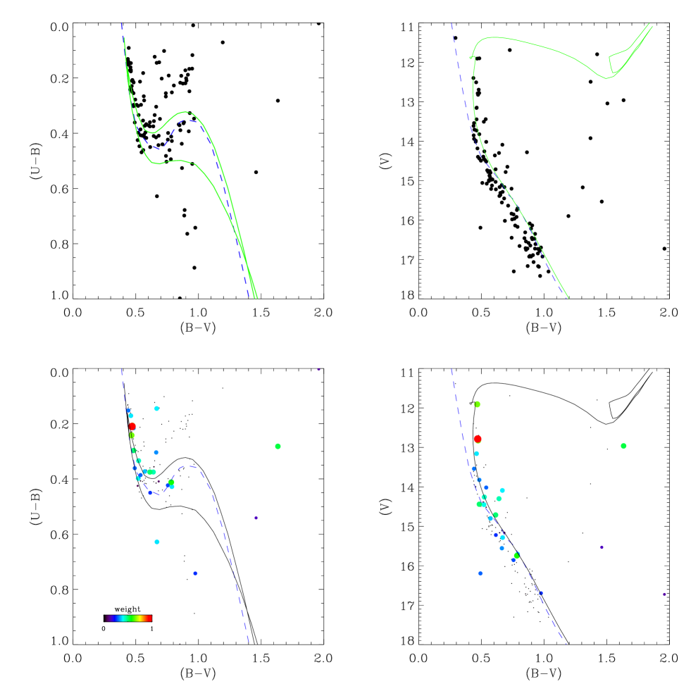
Figure 16: Same as Fig. 4 for Melotte 105 (Ref. 32).

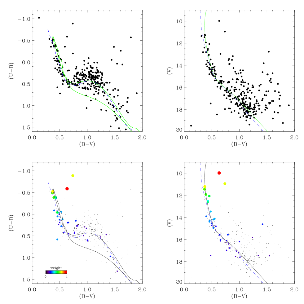
Figure 17: Same as Fig. 4 for Trumpler 1 (Ref. 86).

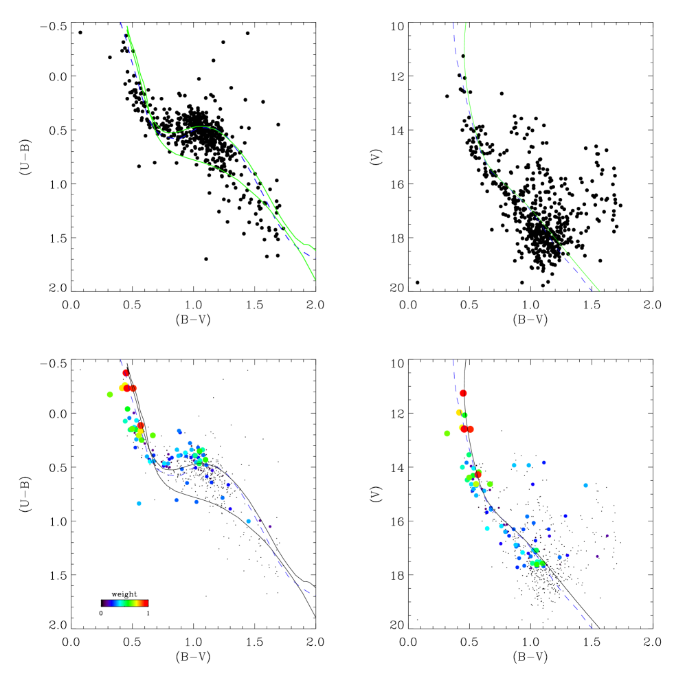
Figure 18: Same as Fig. 4 for Trumpler 1 (Ref. 320).