Mitigating Epidemics through
Mobile Micro-measures
Abstract
Epidemics of infectious diseases are among the largest threats to the quality of life and the economic and social well-being of developing countries. The arsenal of measures against such epidemics is well-established, but costly and insufficient to mitigate their impact. In this paper, we argue that mobile technology adds a powerful weapon to this arsenal, because (a) mobile devices endow us with the unprecedented ability to measure and model the detailed behavioral patterns of the affected population, and (b) they enable the delivery of personalized behavioral recommendations to individuals in real time. We combine these two ideas and propose several strategies to generate such recommendations from mobility patterns. The goal of each strategy is a large reduction in infections, with a small impact on the normal course of daily life. We evaluate these strategies over the Orange D4D dataset and show the benefit of mobile micro-measures, even if only a fraction of the population participates. These preliminary results demonstrate the potential of mobile technology to complement other measures like vaccination and quarantines against disease epidemics.
1 Introduction
Modeling and effectively mitigating the spread of infectious diseases has been a long-standing public health goal. The stakes are high: throughout human history, epidemics have had significant death tolls. In the mid-14 century [15], between 30% and 50% of Europe’s population died due to the Black Death. In 1918, the Spanish flu pandemic caused an estimated 50 million deaths worldwide [33]. More recently, the 2002–2003 SARS pandemic that originated in Hong-Kong and spread worldwide caused the death of 774 [36]. These events highlight not only the scale of the problem but also our vulnerability, past and present. The situation worsens in times of crises. A recent example is the ongoing cholera outbreak in Haiti: it started in 2010, a few months after a major earthquake. Cholera is a recurring issue in West African countries as well, with many deaths reported each time. Effective measures against an epidemic require an accurate and up-to-date assessment of the situation, a very fast response and a strong coordination, which are colossal organizational efforts under tight time constraints. To this day, there is no uncontested way of preventing epidemics in general. Traditionally, many methods that have been used involve top-down approaches such as vaccination campaigns, the set-up of medical shelters, travel restrictions or quarantines [19]. These methods have several drawbacks: they are difficult and slow to be put into place, they can be expensive and also freedom-restrictive. It is clear that any improvement could have a tremendous impact and translate into significant welfare gains.
In our work, we focus on human-mediated epidemics (transmitted by human contact, e.g., influenza). For these epidemics, human mobility clearly plays a crucial role in that it enables the epidemic to travel and spread geographically. We will explore new mitigation methods and expand the solution space. In particular, we argue that taking advantage of mobile technology opens up many possibilities for mitigating the spread of an epidemic in original and distinctive ways. Importantly, mobile technology is unique in that it is allows the personalization of countermeasures through precise measurements at the individual level, as well as individualized recommendations. It is this combination of information extracted from mobile data and subsequent personalization of prevention advice that opens up novel ways of mitigating an epidemic. We envision a mobile service that sends recommendations that invite the individuals to adapt their behavior, for example by delaying or canceling a trip. More generally, we formulate subtle, precise and minimally restrictive personalized behavioral rules that, if followed even partially, will have a positive global effect on the epidemic.
1.1 Context and Contributions
Our work was spurred by the Data for Development challenge111See: http://www.d4d.orange.com/. The challenge was launched in mid-2012 and ended on February 15, 2013. organized by France Telecom-Orange, a global telecommunications operator. Participants in this challenge have access to data gathered from 2.5 billion calls made by 5 million users in Ivory Coast. The goal is to find an original and creative use of this data that contributes towards the social, economic and environmental development of Ivory Coast. Four different datasets were derived from call detail records (CDRs) recorded over a period of 5 months, from December 2011 to April 2012. Blondel et al. [8] provide a detailed description of the datasets. Among these, two are mobility traces containing the time and the location at which a sample of the users made their phone calls. In order to protect the users’ privacy, the datasets reflect different trade-offs in terms of the location’s accuracy and the time span over which the trace is provided. We use this data to build a home location and time-dependent model of human mobility in Ivory Coast, which allows us to accurately capture population movements across the country (Section 4). These mobility patterns then power the core of our epidemic model, which allows us to analyze epidemic outbreaks at the level of single individuals (Section 5).
Beyond these models, our main contribution is to foster the idea of a mobile service that sends personal recommendations to help mitigate an epidemic. The mobile service is an original idea that has several advantages over existing methods. In particular, we introduce and motivate the concept of micro-measures, individual countermeasures tailored to their recipients’ specific behavior; this new approach is the opposite of the one-size-fits-all pattern that characterizes most traditional mitigation measures. We present several concrete such micro-measures and discuss their potential (Section 3). Finally, we empirically evaluate their effectiveness using our epidemic model and provide some insights into further research directions (Section 6).
2 Related Work
Infectious diseases, also known as transmissible diseases are one of the the major causes of deaths in human societies. An epidemic is a rapid and extensive spread of a transmissible disease that affects many individuals in an area, community, or population. In order to study epidemics, scientists need to describe them mathematically, which enables them to predict epidemic outbreaks and to find strategies for decreasing mortality rates, and hence the costs to the economy. In their seminal work, Kermack and McKendrick [23] introduce a SIR model with three distinct classes of populations: susceptibles, infectives and recovered. This simple, yet powerful, model is very popular for modeling the evolution of epidemics in populations. Hethcote [17] reviews different extensions of this model (SIS, SI, SEIS and etc.), as well as threshold theorems involving measures such as the reproduction number, which is the average number of secondary infections caused by an infected individual when in contact with a population of susceptibles.
Instead of modeling an epidemic for the population in a region, it is possible to increase geographical granularity by dividing the original region in sub-regions, and then study the SIR model for the population of each region [1, 5, 26, 34]. By assuming that human contacts are responsible for disease transmission, the disease spread among sub-regions is driven by the mobility of individuals. Sattenspiel and Dietz [26] take into account the home region of individuals in order to simulate their mobility. One of the simple approaches to modeling population mobility is the gravity model that is based on two assumptions: Mobility flux between two regions is proportional to the product of their population’s size. It decays as the distance separating them increases [29]. For example, recently, Rinaldo et al. [25] study the Haiti cholera outbreak (2010–2011) and try to predict the next outbreaks of cholera, using the gravity model and rainfall as drivers of disease transmission. By using a stochastic computational framework, Colizza et al. [9] study the epidemic propagation on a larger scale: They analyse the effect of airline transportation (complete worldwide air travel infrastructure complemented with census population data) on global epidemics.
In order to improve the realism of epidemic models, we need to build more accurate and data-driven mobility models. CDRs collected by cellular services are used for studying human mobility, because they represent a rich source of information about mobility [2, 3, 4, 14, 20, 31]. For example, Gonzalez et al. [14] analyze the trajectory of 100,000 mobile phone users over a six-month period. They find that human trajectories exhibit very regular patterns, hence we can model each individual mobility with only a few parameters. Isaacman et al. [21] model how a large population move within different metropolitan areas. Because of the sporadic nature of CDRs, Ficek and Kencl [12] use a Gaussian mixture model to reproduce probabilistically location of users between two consecutive calls. Based on the number of unique antennas observed by each user, Halepovic and Williamson [16] assume that some proportion of the population are static and always stay in their home regions.
The development of strategies for controlling epidemics such as influenza is one of the high priorities of global public health policies [11, 13, 18, 19]. SIR models, which incorporate mobility between regions, represent powerful tools for designing and testing different strategies to control epidemics. The quarantine is one of the methods often used to limit the spread of infectious diseases within human populations. We lack information however about the effectiveness of quarantine on controlling epidemics. Sattenspiel and Herring [27] use records of the influenza epidemic, which took place in Canada at 1918-19, to investigate the effect of quarantine. They show that a quarantine is effective only when mobility is restricted, and that it depends on its application-time and duration. In addition to these issues about the effectiveness of quarantine, there are issues, that include implementation challenges, economic cost and the violation of civil rights, especially in the cases of long confinement or isolation from society. Another way to control epidemics is to vaccinate the susceptible population in a series of pulses called pulse vaccination [24, 28, 30, 37, 38]. For example, Zaman et al. [37] define a control optimization problem based on the SIR model. They try to compute the optimum percentage of susceptible population to be vaccinated at each time. This method requires the vaccination of at least 10 percent of the susceptible population at each time step, in order to make a small change in the epidemic behaviour of the infectious disease.
3 Mobile Micro-measures
Traditional epidemic mitigation methods consist of heavy, top-down approaches such as blockades, quarantines or large-scale vaccinations. As an alternative, we suggest that mobile technology could enable a much richer and sophisticated set of mitigation measures for human-mediated epidemics, which we name micro-measures. Let us illustrate our vision by describing a simple scenario.
Jean, an 18 year old inhabitant of Ivory Coast living in Northeastern Bouaké, would like to play pickup football. He knows that a meningitis outbreak just surfaced in his district, and he does not want to take any risk. Bouaké happens to be part of a pilot program of a mobile service that helps mitigate the spread of meningitis. Using his mobile phone, he sends a short request to the service that instantly computes the following personalized recommendation for him: to minimize the risk, he should try the football field a few kilometers southwards, instead of going to the one he is used to. It would be best if he took the gbaka (small bus) in about 17 minutes, this way he would avoid contact with the kids coming back home from the school nearby.
Of course, this scenario presents an idealized and naive view of reality; Jean might not have a cell phone to begin with, the bus might not have such a precise schedule, and there might not be alternative locations where people are playing pickup football. It nevertheless gives an overview of the level of refinement that can be achieved through personal recommendations. The main properties of such a service are as follows:
- Personalized.
-
Recommendations are generated and communicated on an individual basis. Mobile technology enables this in two ways: first, it allows for a quantity of valuable behavioral information (such as location and activity) to be recorded and second, it provides a readily available unicast communication channel.
- Adaptive.
-
As the epidemic progresses and each individuals’ intentions are discovered, the recommendations are instantly adapted. The personalization of mobile micro-recommendations ensures their effectiveness. Such recommendations, in contrast with most large-scale mitigation efforts, would typically require much less time to be set up and would always be in phase with the current state of the epidemic.
- Microscopic.
-
In contrast with a one-size-fits-all policy that typically considers an epidemic from a macroscopic perspective, micro-measures tend to focus on subtle and local changes. These changes, when looked at independently, are mostly insignificant; but taken together, they result in important global improvements.
- State-independent.
-
An additional property of the service is that it is epidemic-state independent: the recommendation should not depend on whether the individual is infective or not. First, it does not require prior knowledge about the state of an individual: it is often hard to determine precisely when he becomes infected. Second, it aligns the incentives: without additional knowledge, everyone can expect to benefit from following the recommendation—this might not necessarily be the case when the state is known.
This lays the foundation of our approach but does not yet suggest any concrete mitigation scheme. Still, there are fundamental questions related to the feasibility of micro-measures. Under which conditions do small, local changes (such as an individual agreeing to commute slightly earlier) have a global impact? How many individuals need to cooperate, and how does this, significantly alter the dynamics of the epidemic ? An epidemic can often be seen as being either supercritical (the epidemic grows) or subcritical (it declines). What microscopic changes are susceptible to cause a phase transition? Although a precise characterization of these changes and, by extension, rigorous answers to these questions are beyond the scope of our work, we intend to show initial evidence of the relevance of such a mobile service.
3.1 Concrete Micro-Measures
Beyond a theoretical argument, our contribution is the description and evaluation of three concrete strategies we can use to generate micro-measures. They represent initial baselines for further developments. Let us first note that contacts between individuals can broadly be categorized into two groups: the deliberate contacts are, for example, between family members or at work, whereas the accidental contacts are formed by random encounters, for instance, while shopping or commuting. At a high level, our approach is to maintain deliberate contacts and rewiring the accidental ones. The idea is to weaken the links in the contact network that form the path through which the epidemic spreads. By changing its structure, we seek to decelerate the dynamics and drive the epidemic down to a sub-critical level.
| CutCommunities | DecreaseMix | GoHome | |
|---|---|---|---|
| Knowledge to maintain | List of communities of locations | Social communities of users | State of the epidemic across regions |
| Recommendation | Do not cross community boundaries | Stay with your social circle | Go/stay home |
| Intuition | Weakening the weak geographical links | Segmenting social communities | Home is a safe place |
3.1.1 CutCommunities strategy
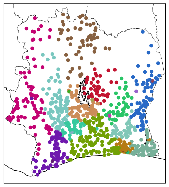
It is clear that mobility drives the spread of an epidemic. A straightforward strategy would therefore be to reduce long-range contacts, be it at the expense of reinforcing local ones. Uniformly reducing mobility is, however, both expensive and inflexible. To overcome this, our first strategy, CutCommunities, takes into account communities of locations in the mobility network, and focuses on reducing human mobility over inter-community links—this is, in a sense, analogous to weakening the weak links in the network. The main difference with a simple blockade is that our strategy is able to adapt to changes in the network (mobility patterns vary over time, cf. Section 4). In practice, the service operator would maintain a list of location communities identified through the mobility patterns of its userbase; when an individual checks whether a trip is safe, the service would verify whether it crosses community boundaries and, if this is the case, discourage the individual from making this trip222As a relaxation of this counter-measure, we could consider postponing the trip instead. Simply by delaying certain trips, we could prevent harmful interactions between groups of individuals. This is analogous to time-division multiplexing; a slight change in the habits of a group of people might significantly change the contact surface.. If additional per-location information is available about the current state of the epidemic, recommendations could be further corrected according to the strength of the epidemic at the individual’s current and projected locations.
3.1.2 DecreaseMix strategy
Instead of acting on mobility to segment contacts across location communities, we also consider segmentation social communities. The aim is to separate individuals inside the same location, e.g., by making them visit different aisles of the same supermarket at different times. Putting in place such a segmentation is more sophisticated than in the case of mobility, but this strategy is the perfect example of another extremal point in the solution space. The service operator would keep a list of social communities and would communicate a distinctive tag (e.g., a color) to individuals according to their community. Individuals would access locations differently, depending on their tag; for example, seating in a theater would be organized in such a way that contacts between communities are minimized. We are aware that this strategy could raise many concerns, because it segregates people, therefore great care would be needed if it were to be implemented. Despite this, we retain it because it reflects a different trade-off with respect to CutCommunities: instead of discouraging individuals from going to certain locations where they can be in contact with everyone, we allow them go everywhere, but restrict the contact network.
3.1.3 GoHome strategy
We consider a third case where the service recommends individuals to go home. The intuition behind this strategy is that we assume that when at home, the contact rate decreases. Whereas the previous strategies target the individuals’ location or contact network, this one is distinctive in that it affects the the rate of contact. With information on the progress of the epidemic across locations, the operator could prioritize sending advice to those individuals whose cooperation would yield the greatest effect. In Section 6, we will provide a detailed evaluation of the three described strategies. Before doing so, we will introduce the mobility and epidemic models used for our assessments.
4 Mobility Model
Because the spread of epidemics depends greatly on the mobility of infected individuals, and on the locations where they interact with other individuals, a realistic, data-driven mobility model is a essential tool for simulating realistic epidemic propagation. It should therefore model population mobility, take into account certain microscopic aspects at the individual level, and still allow simulations of epidemic propagation to scale up to millions of individuals. Moreover, it should capture the main differences between the mobility of different groups of individuals, where a group is constituted of individuals exhibiting similar mobility profiles. To construct a mobility model that fulfils these requirements, our intuition is : The home location of individuals strongly shapes their mobility patterns because the places they visit regularly e.g., their workplaces, schools or the shopping centers, depend on the proximity to their home. Typically, we expect the most visited location (home) and the second most visited location (school, university or work) to be geographically close to each other. In addition to this geographical aspect, mobility is strongly time-dependent: Individuals commute between home and work during the weekdays, with a substantial change in their travel behavior during the weekends.
| Definition | Domain | Explanation |
|---|---|---|
| = {1, …, 1231} | - | Set of antennas |
| = {1, …, 255} | - | Set of sub-prefectures |
| Time resolution | ||
| Home sub-prefecture | ||
| Home antenna | ||
| Antenna | ||
| Absolute time | ||
| Period of the day | ||
| = day() | Day of the week | |
| = weekday() | Day type: weekday or weekend |
Building on this, we make the assumption that the individuals that share the same home-location exhibit a similar mobility pattern. Therefore, we construct a location and time-based mobility model that depends on the variables presented in Table 2. The conditional distribution of the location of user depends on his home antenna , but also on the time of the visits :
| (1) |
First, we choose the the time resolution in order to divide the day in 3 distinct periods: Morning (6 am to 1 pm), afternoon (1 pm to 8 pm) and night (8 pm to 6 am). Second, conditioning on the parameter allows us to distinguish between weekdays and weekends. Finally, the home antenna of user is defined as the most visited antenna during the night period. Consequently, given the period of the day, the day type and the home antenna of user , the distribution of the location that he might visit (1) is a multinomial distribution with categories.
4.1 Learning and Evaluating Mobility Models
In order to build our model from data, we analyse SET2, one of the datatsets provided by France Telecom-Orange [8]. It contains high-resolution trajectories of 500,000 users, observed over a two-week period. We focus on this datatset, as it offers the highest geographical resolution : Individuals’ locations are observed across antennas. To avoid having to deal with users whose location samples are very sparse, we consider only the users who visited more than 1 antenna and made on average more than 1 call per day. In order to evaluate the realism of our mobility model, we separate the data into two parts: For each user, we put of the calls in the training set and the remaining in the test set. First, we build a mobility model by learning from the training set by using a maximum likelihood estimator . Then, we evaluate our mobility model by computing the average log-likelihood of the calls belonging to the unseen test set. The average log-likelihood reflects how well our model generalizes to unseen data. As the test set might contain some locations not visited by a given class of users in the training set, the maximum likelihood estimate of the distribution (1) assigns zero probability to these observations. We cope with this by assuming that the distribution (1) is a multinomial distribution drawn from an exchangeable Dirichlet distribution, which implies that the inferred distribution (1) is a random variable drawn from a posterior distribution conditioned on the training data. A more detailed description of this smoothing procedure is given by Blei et al. [6].
We tested several variants of mobility models by varying their structure and parameters (time resolution, day of the week, etc). To have three representative baseline models for comparison, we choose three predictors out of the several variants we tested.
The first baseline model is a time-based mobility (TM) model
| (2) |
where all mobile-phone users exhibit the same time-dependant geographical distribution. The second baseline is a location-dependent first order Markov chain (MC)
| (3) |
where the current location of a user depends only the location he visited just before. The third baseline is a time and sub-prefecture dependant mobility model (SPM)
| (4) |
where the home of a user is represented by a sub-prefecture instead of an antenna. This implies a more important aggregation of users, where two users who share the same home sub-prefecture, have the same mobility pattern.
| Mobility model | Average log-likelihood |
|---|---|
| Our model | -1.07 |
| SPM | -1.67 |
| TM | -2.9 |
| MC | -6.49 |
The experimental results are shown in Table 3. The first order Markov chain (MC) performs the worst. This is not surprising since the time difference between two call records varies greatly, ranging from a few minutes to a few days. The location associated with a call made in the past few hours or days does not necessarily affect the current location. As the location data is sporadic, it is not surprising than any model that learns from transitions performs poorly, and is outperformed by time-based models. Our model performs the best; and by comparing it to the time-based model (TM), we realise that knowing the home-locations of users enhances the predictive power of the mobility model. Moreover, the granularity of home locations is crucial: Our model significantly outperforms the sub-prefecture dependent mobility model because it has a finer granularity of the home-location.
A realistic mobility model is an essential building block of a realistic epidemic propagation model because mobility drives population flows between regions, and therefore the geographical proximity between individuals. In the next section, we introduce the epidemic model we use to simulate a local epidemic propagation.
5 Epidemic Model
Building up on the mobility, this section introduces our epidemic model. It is based on a discretized, stochastic version of the SIR model [23]; Tables 4 and 5 provide an overview of the different parameters and quantities used throughout the section. We assume that the size of the population ( individuals) remains constant—there are no births nor deaths, a reasonable assumption if the time horizon is limited to at most a few months. Under the SIR model, an individual can be either susceptible to the disease, infective, or recovered from the disease and immunized against further infections333In the literature, this state is sometimes known as removed. The important point is that they do not participate in the epidemic anymore.. We assume that most of the population is initially susceptible, except for a small number of infective individuals that form the seed of the epidemic. Individuals successively go through the susceptible, infective and recovered states; a desirable outcome would have many individuals stay susceptible without ever becoming infective. The basic SIR model assumes random mixing of the whole population: any individual meets any other one with a uniform probability. In our model, we relax this strong assumption by taking into account the mobility. We spread the population across regions; each region bears its own SIR process where the corresponding meta-population mixes at random. These regional processes are independent and isolated, and the only way the epidemic crosses regional boundaries is through human mobility [22]. In summary, regional interactions take place uniformly at random, whereas global interactions are shaped by the individuals’ mobility.
| total population | |
| number of regions | |
| initial population of region , where | |
| number of different mobility classes | |
| contact probability | |
| recovery probability |
| mobility class , where | |
| distribution of the number of susceptible individuals in region across classes. | |
| distribution of the number of infected individuals in region across classes. | |
| distribution of the number of recovered individuals in region across classes. | |
| number of susceptible individuals in region , equal to | |
| number of infected individuals in region , equal to | |
| number of recovered individuals in region , equal to | |
| population of region , where | |
| infection probability for region . |
5.1 Local Epidemic Dynamics
In order to work at the individual level, we adapt the classic deterministic SIR model in order to have a discrete-time stochastic variant. The contact probability and recovery probability are constant across all regions444These quantities are rates in the continuous time SIR model. In order to carry over the characteristics of the SIR model to our discretized version, we need to ensure that the sampling interval is short enough to ensure that .. For a region we compute, at each time step, the force of infection . This quantity represents the probability of making a contact that results in an infection. During a time step, every susceptible individual gets infected independently at random with probability , while every infective individual recovers independently at random with probability . If we denote by the variation of after one time step, it is easy to see that
which are the expected difference equations for the SIR model under the random mixing assumption. We note that our model has many similarities with that of Colizza et al. [10], used to model the SARS pandemic.
5.2 Implementation
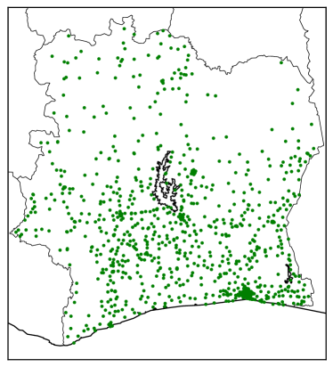
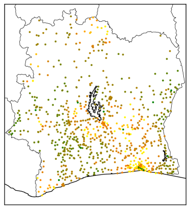
To allow for distinctive mobility patterns across the population, individuals belong to one out of classes that fully characterize their mobility patterns. In accordance with the mobility model (Section 4), the individuals’ class is determined by their home antenna. The implementation is best understood when decomposed into two distinct, successive phases: a mobility phase where individuals can move between regions, and an epidemic phase where individuals get infected or recover.
- Mobility phase
-
We consider every individual. Suppose the individual is in region ; the mobility model assigns a new region according to its mobility class. If we update the vectors and accordingly, where depends on the current state of the individual.
- Epidemic phase
-
We consider every region . We begin this phase by updating the infection rate given the current values of and . Every infected individual then recovers with probability , while every susceptible individual gets infected with probability . , and are updated accordingly.
This process is repeated until the end of the period of interest.
6 Empirical Evaluation
Next, we use our models to test the strategies previously described in Section 3. Before evaluating our strategies, we first explain how the epidemic model is parameterized and how epidemic spreads are quantitatively characterized.
6.1 Model Parameters and Evaluation Metrics
In order to be consistent with our mobility model, the epidemic model defines regions to be the area surrounding the antennas (). Hence, we will use the words region and antenna interchangeably. As an individual’s mobility is tied to his home antenna, we distinguish among different classes. To initialize the population attached to each antenna, we use data from the AfriPop project [32] which provides us with Ivory Coast population figures at the hectare level; to account for the fact that not every individual is mobile, we allow only 55% of the population to move during the mobility phase555This distinction is rather crude and could certainly be further refined. However we deemed it to be sufficient for our purposes., which roughly corresponds to the proportion of the population in the 15-to-64 age bracket [35]. Days are divided into three time steps in order to match the mobility model666Notice that this is not a formal requirement. We use this subdivision mainly for simplicity., and the typical time horizon is between 100 and 400 time steps (i.e. 1–4 months). Contact and recovery probability are usually set to , respectively ; Although these synthetic values do not directly match any well-known disease, they are still qualitatively close to realistic cases, such as influenza. All our simulations start with a seed set of 23 infectives distributed across 5 antennas777In the datasets provided by France Telecom-Orange, these antennas have the following identifiers: 57, 146, 330, 836, 926. in the Attécoubé district of Abidjan.
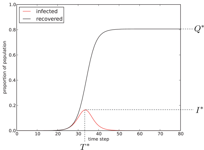
In order to quantify the difference between epidemic spreads, we propose three metrics to evaluate the effectiveness of our mitigation strategies. Figure 3 shows how these quantities are related to the epidemic’s evolution over time. For notational clarity, let be the total number of individuals in each state over the country as a whole. As these quantities evolve over time, they are functions of the time step . The first metric is the size of the largest outbreak or, equivalently, the maximal proportion of infective individuals,
The reasoning behind this metric is self-evident: in most cases, the larger the proportion of infective individuals, the more difficult the control of the epidemic. It is also, broadly speaking, a good indicator of the epidemic’s strength. Our second metric is closely related to the first one, but considers the complementary dimension: it measures the time of the largest outbreak,
Delaying the moment at which the epidemic reaches its peak allows individuals and governments to have enough time to adapt their behavior, respectively, to deploy measures. Finally, our last metric captures the tail behavior of the epidemic: it measures the final proportion of recovered users,
Note that we would like to minimize this metric. After the epidemic dies out, all individuals are either recovered or susceptible, and a low proportion of recovered individuals means that a high percentage of the population did not go through the infective state at all.
6.2 Results
We now take a closer look at our three proposed strategies. We will describe how we instantiate them and we provide qualitative and quantitative assessments with respect to their effectiveness.
6.2.1 CutCommunities strategy
| Affected movements | Maximum | |
|---|---|---|
| () | ||
| () | ||
| () |
The first strategy divides the country into location communities according to the network of mobility. We consider the weighted, undirected graph where nodes represent antennas, and edge weight is equal to the average number of trips between the two endpoints (regardless of direction). We use the Louvain community detection algorithm [7]; Figure 1 shows the 30 identified communities. It is interesting—but not surprising—to note that the communities are roughly geographicaly based888As a sidenote, we ran the Louvain method on a number of other graphs generated from the datasets provided for the D4D challenge, including one derived from SET1 representing total antenna-to-antenna communications. The communities always displayed the same geographical clustering. Furthermore, we observed that mobility communities seem to be correlated to phone call communities.. This confirms our hypothesis stating that there are geographical weak links. Micro-measures are then generated as follows: when an individual checks whether a trip is safe, the service first verifies whether the trip crosses community boundaries and whether the current or projected locations are affected by the disease; if both of these conditions are met, the individual is discouraged from making the trip. The recipient then complies with probability .
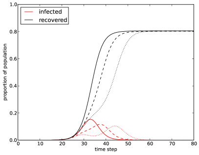
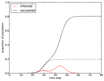
Figure 4 shows the effect of CutCommunities for different values of . Compared to the baseline (), the strategy affects the size and the time of the epidemic’s peak. However, it does not change much the tail behavior: stays constant at around , except for the degenerate case where , which represents a blockade around the community initially infected. We also observe that there seem to be two infection phases, made progressively more apparent as , and that the blockade removes the second phase; these two phases correspond to infections happening inside, respectively, outside the initially infected community. Recall that this strategy only sends micro-measures to a fraction of the individuals, those who cross community boundaries—a case that by definition should not happen too often. It is therefore interesting to consider the number of trips actually canceled as a result: Table 6 lists the average and maximal proportion for different values of . The numbers are quite low999That these proportions are lowest when is due to the fact that the epidemic is local to the infective seeds’ community, suggesting that the communities form a natural partitioning of the regions. In conclusion, this strategy does not affect the asymptotic behavior of the epidemic but significantly shifts its peak. Altogether, it justifies the relevance of mobility-based geographical communities as a data source to generate micro-measures.
6.2.2 DecreaseMix strategy
Recall that this strategy assigns tags to individuals according to the social community to which they belong and segregates contacts across social communities. A service operator might use the call graph (i.e. the social network derived from who calls whom) to infer social communities in the population; unfortunately, we do have access to such data101010The data provided for the Orange D4D challenge does include a dataset consisting of myopic views of the call graph. SET4 is a sample of egonets, i.e. balls of radius two centred at a particular user. However, this dataset did not yield anything useful for our purposes.. In order to quantify the effectiveness this strategy, we proceed as follows. Similarly to our mobility model, we make the assumption that the individual’s community is determined by his home antenna. The DecreaseMix strategy do not decrease the total number of contacts; instead it rewires contacts across communities to contacts inside the community. This is done by splitting the contact probability to into intra-community and inter-community contact probabilities and introducing a mixing parameter
where indicates the number of individuals of community currently in region , and the other quantities follow the same convention of notation. The intuition is as follows: When , everyone mixes at random inside a region just as if no countermeasure was applied at all. At the other extreme, when , contacts happen only with individuals from the same community. Intermediary values of allow us to play with the strength of the segregation.
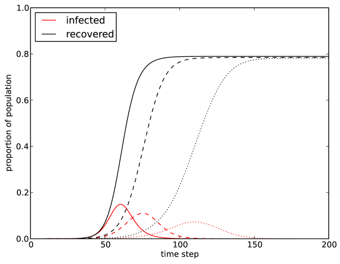
We evaluate the effectiveness of DecreaseMix for different values of the mixing parameter . Our simulations are parameterized with , and ; Figure 5 shows the average behavior of the epidemic over 10 runs. The main characteristic of this strategy is that it delays the epidemic outbreak. However, the slopes of the two curves at the strongest point of the epidemic are not very differentiated. As s result, the final proportion of recovered does not vary much. But by making it 10 or 100 times more likely to contact an individual of the same community, we delay by approximately 5 and 16 days, respectively, on average. Our intuition about this phenomenon is that it takes more time for the epidemic to reach certain communities (as they are more segregated), but once a community sees its first case of infection, the spread is just as fast as before. We argue that one of the main limiting factors at play here is the random mixing assumption: if we were able to bring finer structural changes to the contact graph, the situation would look very different.
6.3 GoHome strategy
| Affected movements | Maximum | |
|---|---|---|
| () | ||
| () |
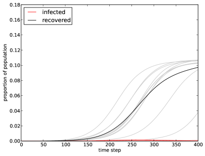
Our last strategy advices individuals to go home or stay home. In order to focus the micro-measures on the most influential individuals, we assume that at each time step, the service operator knows the proportion of susceptible, infective and recovered individuals across locations. We suppose that before every trip, an individual sends a request to the service that compares the proportion of infectives in both source and destination, and recommends to go home if the destination has a proportion of infectives, lower than the source location. Individuals then comply with probability . The main intuition behind this choice is to avoid sending infective individuals to highly susceptible locations. Note that we keep the state-independent assumption here: we do not know the state of the individual when sending out a recommendation. The second important assumption is that, when the individual is at at home, the contact probability is set to be equal to the recovery probability111111When contact and recovery probability are equal, the single-population SIR epidemic (under the random mixing assumption) does not develop anymore; setting can therefore be seen as the least change needed to stabilize the epidemic., i.e. . This models the fact that there are less contacts at home, in term of accidental ones. Mixing is not exactly uniform anymore, and the infection probability is adapted as follows:
Quantities with loc and vis subscripts correspond to individuals whose home region is (respectively is not) . Note that the contact probability of visitors can significantly decrease in a region where the proportion of visitors to locals is low.
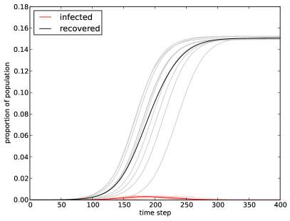
This time, the effectiveness depends on the value of the compliance probability . We use again , and let ; Figure 6 shows the behavior of the epidemic over 10 runs. As opposed to the results obtained with the DecreaseMix strategy, we obtain significant improvements to as increases121212Unfortunately, our simulation was limited to time steps, which is not enough to clearly show the asymptotical behavior. The claim, however, is justified by looking at the worst runs whose slope quickly tends to zero.. This observation is not surprising because by suggesting to individuals to go home, we are directly reducing their contact probability, which is a determining factor of the epidemic’s dynamics. It is also interesting to look at the actual number of trips that are affected (i.e., cancelled) because of the micro-measures; Table 7 shows that a relatively low number of trips have to be affected to noticeably impact the spread. In summary, this strategy has the potential to be quite effective, although the assumptions it makes deserve closer analysis.
7 Conclusion
In this paper, we explore the novel idea of using mobile technology in order to mitigate the spread of human-mediated infectious diseases. We motivate the concept of mobile micro-measures that consist of personalized behavioral recommendations given to individuals. By affecting, even partially, individual behaviors, we are able to globally impact the epidemic propagation. These mobile micro-measures have several original properties; they are adaptive, target individuals at the microscopic level and provide a rich set of mitigation methods. Using the data provided for the Orange D4D challenge [8], we first develop a realistic mobility model for the population of Ivory Coast. Then, we incorporate it into an epidemic model based on SIR in order to simulate the epidemic propagation, while taking into account population mobility. Taking advantage of this framework, we propose and evaluate three concrete strategies used to generate micro-measures. Our strategies weaken the epidemic’s intensity, successfully delay its peak and, in one case, significantly lower the total number of infected individuals.
These preliminary results allow us to identify several research avenues. First, random mixing is the most limiting assumption. Being able to change the structure of human contacts at a finer level is a key component of more advanced micro-measures. The mobile call graph is an example of a source of information about social contacts, one that is readily available to mobile phone operators. Second, beyond our preliminary strategies, it is highly important to deepen our understanding of the key ingredients that make mobile micro-measures effective yet minimally restrictive. In parallel to mobile micro-measures, the availability of large-scale mobility data opens up new research directions in epidemiology: a more precise characterization of the relation between epidemic spread and human mobility patterns is an interesting topic we would also like to investigate in the future.
To conclude, we firmly believe that data-driven and personalized measures which take advantage of mobile technology are an important step towards effective epidemic mitigation.
Acknowledgements
We would like to thank Vincent Etter for his insightful comments and feedback about this paper.
References
- Arino and Van den Driessche [2003] J. Arino and P. Van den Driessche. A multi-city epidemic model. Mathematical Population Studies, 10(3):175–193, 2003.
- Barabasi [2005] A.-L. Barabasi. The origin of bursts and heavy tails in human dynamics. Nature, 435(7039):207–211, 2005.
- Bayir et al. [2009] M. A. Bayir, M. Demirbas, and N. Eagle. Discovering SpatioTemporal Mobility Profiles of Cellphone Users. In WoWMoM 2009, pages 1–9. IEEE, 2009.
- Becker et al. [2013] R. Becker, R. Cáceres, K. Hanson, S. Isaacman, J. M. Loh, M. Martonosi, J. Rowland, S. Urbanek, A. Varshavsky, and C. Volinsky. Human Mobility Characterization from Cellular Network Data. Communications of the ACM, 56(1):74–82, 2013.
- Belik et al. [2009] V. Belik, T. Geisel, and D. Brockmann. The impact of human mobility on spatial disease dynamics. In CSE 2009, volume 4, pages 932–935. IEEE, 2009.
- Blei et al. [2003] D. M. Blei, A. Y. Ng, and M. I. Jordan. Latent Dirichlet Allocation. Journal of Machine Learning Research, 3:993–1022, 2003.
- Blondel et al. [2008] V. Blondel, J. Guillaume, R. Lambiotte, and E. Lefebvre. Fast unfolding of communities in large networks. Journal of Statistical Mechanics: Theory and Experiment, 2008(10):P10008, 2008.
- Blondel et al. [2012] V. D. Blondel, M. Esch, C. Chan, F. Clerot, P. Deville, E. Huens, F. Morlot, Z. Smoreda, and C. Ziemlicki. Data for Development: the D4D Challenge on Mobile Phone Data. arXiv preprint arXiv:1210.0137, 2012.
- Colizza et al. [2006] V. Colizza, A. Barrat, M. Barthélemy, and A. Vespignani. The role of the airline transportation network in the prediction and predictability of global epidemics. PNAS, 103(7):2015–2020, 2006.
- Colizza et al. [2007] V. Colizza, A. Barrat, M. Barthélemy, and A. Vespignani. Predictability and epidemic pathways in global outbreaks of infectious diseases: the SARS case study. BMC Medicine, 5(34), 2007.
- Ferguson et al. [2006] N. M. Ferguson, D. A. Cummings, C. Fraser, J. C. Cajka, P. C. Cooley, and D. S. Burke. Strategies for mitigating an influenza pandemic. Nature, 442(7101):448–452, 2006.
- Ficek and Kencl [2012] M. Ficek and L. Kencl. Inter-Call Mobility Model: A Spatio-temporal Refinement of Call Data Records Using a Gaussian Mixture Model. In INFOCOM 2012, pages 469–477. IEEE, 2012.
- Germann et al. [2006] T. C. Germann, K. Kadau, I. M. Longini Jr, and C. A. Macken. Mitigation strategies for pandemic influenza in the United States. PNAS, 103(15):5935–5940, 2006.
- Gonzalez et al. [2008] M. C. Gonzalez, C. A. Hidalgo, and A.-L. Barabasi. Understanding individual human mobility patterns. Nature, 453(7196):779–782, 2008.
- Gottfried [1985] R. Gottfried. Black Death. Simon and Schuster, 1985.
- Halepovic and Williamson [2005] E. Halepovic and C. Williamson. Characterizing and Modeling User Mobility in a Cellular Data Network. In Proc. Workshop on PE-WASUN 20, pages 71–78. ACM, 2005.
- Hethcote [2000] H. W. Hethcote. The Mathematics of Infectious Diseases. SIAM review, 42(4):599–653, 2000.
- Hufnagel et al. [2004] L. Hufnagel, D. Brockmann, and T. Geisel. Forecast and control of epidemics in a globalized world. PNAS, 101(42):15124–15129, 2004.
- Inglesby et al. [2006] T. Inglesby, J. Nuzzo, T. O’Toole, and D. Henderson. Disease Mitigation Measures in the Control of Pandemic Influenza. Biosecurity and Bioterrorism: Biodefense Strategy, Practice, and Science, 4(4):366–375, 2006.
- Isaacman et al. [2011] S. Isaacman, R. Becker, R. Cáceres, S. Kobourov, M. Martonosi, J. Rowland, and A. Varshavsky. Ranges of Human Mobility in Los Angeles and New York. In PERCOM 2011, pages 88–93. IEEE, 2011.
- Isaacman et al. [2012] S. Isaacman, R. Becker, R. Cáceres, M. Martonosi, J. Rowland, A. Varshavsky, and W. Willinger. Human Mobility Modeling at Metropolitan Scales. In MobiSys 2012, pages 239–252. ACM, 2012.
- Keeling et al. [2010] M. J. Keeling, L. Danon, M. C. Vernon, and T. A. House. Individual identity and movement networks for disease metapopulations. PNAS, 107(19):8866–8870, 2010.
- Kermack and McKendrick [1927] W. Kermack and A. McKendrick. A contribution to the mathematical theory of epidemics. Proceedings of the Royal Society A, 115:700–721, 1927.
- Meng and Chen [2008] X. Meng and L. Chen. The dynamics of a new SIR epidemic model concerning pulse vaccination strategy. Applied Mathematics and Computation, 197(2):582–597, 2008.
- Rinaldo et al. [2012] A. Rinaldo, E. Bertuzzo, L. Mari, L. Righetto, M. Blokesch, M. Gatto, R. Casagrandi, M. Murray, S. M. Vesenbeckh, and I. Rodriguez-Iturbe. Reassessment of the 2010–2011 Haiti cholera outbreak and rainfall-driven multiseason projections. PNAS, 109(17):6602–6607, 2012.
- Sattenspiel and Dietz [1995] L. Sattenspiel and K. Dietz. A Structured Epidemic Model Incorporating Geographic Mobility Among Regions. Mathematical Biosciences, 128(1):71–91, 1995.
- Sattenspiel and Herring [2003] L. Sattenspiel and D. A. Herring. Simulating the Effect of Quarantine on the Spread of the 1918–19 Flu in Central Canada. Bulletin of Mathematical Biology, 65(1):1–26, 2003.
- Shulgin et al. [1998] B. Shulgin, L. Stone, and Z. Agur. Pulse Vaccination Strategy in the SIR Epidemic Model. Bulletin of Mathematical Biology, 60(6):1123–1148, 1998.
- Simini et al. [2012] F. Simini, M. C. González, A. Maritan, and A.-L. Barabási. A universal model for mobility and migration patterns. Nature, 484(7392):96–100, 2012.
- Stone et al. [2000] L. Stone, B. Shulgin, and Z. Agur. Theoretical Examination of the Pulse Vaccination Policy in the SIR Epidemic Model. Mathematical and Computer Modelling, 31(4):207–215, 2000.
- Tanahashi et al. [2012] Y. Tanahashi, J. R. Rowland, S. North, and K.-L. Ma. Inferring Human Mobility Patterns from Anonymized Mobile Communication Usage. In MoMM 2012, pages 151–160. ACM, 2012.
- Tatem, A.J. [2010] Tatem, A.J. Côte d’Ivoire AfriPop Data 2010 (alpha version). Emerging Pathogens Institute, University of Florida, 2010. URL http://www.clas.ufl.edu/users/atatem/index_files/CIV.htm.
- Taubenberger and Morens [2006] J. Taubenberger and D. Morens. 1918 Influenza: The mother of all pandemics. Rev Biomed, 17:69–79, 2006.
- Truscott and Ferguson [2012] J. Truscott and N. M. Ferguson. Evaluating the Adequacy of Gravity Models as a Description of Human Mobility for Epidemic Modelling. PLOS Computational Biology, 8(10):e1002699, 2012.
- United Nations, Department of Economic and Social Affairs [2010] United Nations, Department of Economic and Social Affairs. World Population Prospects, the 2010 Revision, 2010. URL http://esa.un.org/unpd/wpp/index.htm.
- World Health Organization [2004] World Health Organization. Summary of probable SARS cases with onset of illness from 1 November 2002 to 31 July 2003, 2004. URL http://www.who.int/csr/sars/country/table2004_04_21/en/index.html.
- Zaman et al. [2008] G. Zaman, Y. Han Kang, and I. H. Jung. Stability analysis and optimal vaccination of an SIR epidemic model. BioSystems, 93(3):240–249, 2008.
- Zaman et al. [2009] G. Zaman, Y. H. Kang, and I. H. Jung. Optimal treatment of an SIR epidemic model with time delay. BioSystems, 98(1):43–50, 2009.