In-flight calibration and verification of the Planck-LFI instrument

Abstract

In this paper we discuss the Planck-LFI in-flight calibration campaign. After a brief overview of the ground test campaigns, we describe in detail the calibration and performance verification (CPV) phase, carried out in space during and just after the cool-down of LFI. We discuss in detail the functionality verification, the tuning of the front-end and warm electronics, the preliminary performance assessment and the thermal susceptibility tests. The logic, sequence, goals and results of the in-flight tests are discussed. All the calibration activities were successfully carried out and the instrument response was comparable to the one observed on ground. For some channels the in-flight tuning activity allowed us to improve significantly the noise performance.

1 Introduction

The Low Frequency Instrument (LFI) is an array of 22 coherent differential receivers in Ka, Q and V bands on board the European Space Agency Planck satellite [1, 2]. The LFI shares the Planck telescope focal plane with the High Frequency Instrument (HFI), a bolometric array in the 100-857 GHz range cooled to 0.1 K [3]. The Planck  full-sky measurements from the Lagrangian point L2 will provide cosmic variance- and foreground-limited measurements of the Cosmic Microwave Background (CMB) by scanning the sky in almost great circles with a 1.5 m dual reflector aplanatic telescope [4, 5, 6, 7].

After being successfully launched on May, 14^th 2009 with the infrared Herschel satellite, Planck was transferred to its final orbit around L2. A series of tests were performed during the first three months in the so-called calibration, performance and verification (CPV) phase, aimed at verifying functionality, tuning of instrument parameters and assessing calibration and scientific performance. Since the start of nominal operations, Planck has scanned the entire sky seven times and has started the eighth survey as we write. The measured LFI and HFI in-flight scientific performance meets all ground expectations making Planck the most sensitive CMB space experiment to date [8, 9].

In this paper we discuss the strategy adopted for the Planck-LFI CPV campaign and provide detailed results of tuning, calibration, and verification tests that were key in meeting the challenging design performance. The cryogenic nature of the spacecraft and instrument required a rather complex operation scheme. This paper, therefore, may constitute a valuable source of information and experience for the execution of in-flight calibration campaigns in future CMB space missions.

After a brief overview of the LFI instrument (see Section 2), in Section 3 we give an overview of the LFI test campaigns, of the cooldown sequence, and of the CPV rationale. Then in Section 4, the heart of this paper, we discuss in detail the methodology and results of the main tests performed on LFI during the CPV phase. Summary and conclusions are provided in Section 5.

2 Overview of the Planck-LFI Instrument

2.1 Receiver schematics and signal model

The Planck-LFI instrument is an array of 11 radiometric receivers in the Ka, Q and V bands, with centre frequencies close to 30, 44 and 70 GHz. The exact centre frequencies for each receiver are reported in [8]; for simplicity, in this paper we will refer to the three channels using their nominal centre frequency. A detailed description of the LFI instrument is given in [10], and references therein. Here we outline the main instrument features that are essential for a self-consistent discussion of the CPV tests.

The instrument (Figure 1) consists of a $20$ K focal plane unit (FPU) hosting the corrugated feed horns, the orthomode transducers (OMTs) and the receiver front-end modules (FEMs). Fourty four composite waveguides [11] are interfaced with three conical thermal shields and connect the front-end modules to the warm ($\sim 300$ K) back-end unit (BEU) containing a further radio frequency amplification stage, detector diodes and all the electronics for data acquisition and bias supply. Every radiometer chain assembly (RCA) consists of two radiometers, each feeding two diode detectors (Figure 2), for a total of 44 detectors. The 11 RCAs are labelled by a numbers from 18 to 28 as outlined in the right panel of Figure 1.

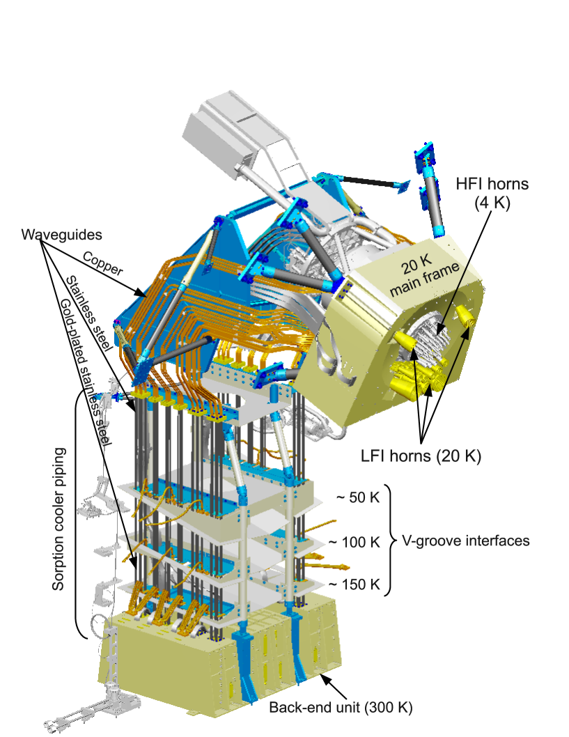
Figure 1: Left panel: the LFI instrument with main thermal stages, focal plane, waveguides and sorption cooler piping highlighted. Right panel: labelling of feed horns on the LFI focal plane.

Figure 2 provides a more detailed description of each radiometric receiver. In each RCA, the two perpendicular linear polarisation components split by the OMT propagate through two independent pseudo-correlation differential radiometers, labelled as M or S depending on the arm of the OMT they are connected to (“Main” or “Side”, see lower-left inset of Figure 2). In each radiometer the sky signal coming from the OMT output is continuously compared with a stable 4 K blackbody reference load mounted on the external shield of the HFI 4 K box [12]. After being summed by a first hybrid coupler, the two signals are amplified by $\sim 30$ dB, see upper-left inset of Figure 2. The amplifiers were selected for best operation at low drain voltages and for gain and phase match between paired radiometer legs, which is crucial for good balance. Each amplifier is labelled with codes 1, 2 so that the four outputs of the low noise amplifiers (LNAs) can be named with the sequence: M1, M2 (radiometer M) and S1, S2 (radiometer S). Tight mass and power constraints called for a simple design of the data acquisition electronics (DAE) box so that power bias lines were divided into five common-grounded power groups with no bias voltage readouts; only the total drain current flowing through the front-end amplifiers is measured and is available to the house-keeping telemetry. A phase shift alternating between 0^∘and 180^∘at the frequency of 4 kHz is applied in one of the two amplification chains and then a second hybrid coupler separates back the sky and reference load components that are further amplified and detected in the warm BEU, with a voltage output ranging from $-$2.5 V to $+$2.5 V. Each radiometer has two output diodes which are labelled with binary codes 00, 01 (radiometer M) and 10, 11 (radiometer S), so that the four outputs of each radiometric chain can be named with the sequence: M-00, M-01, S-10, S-11.

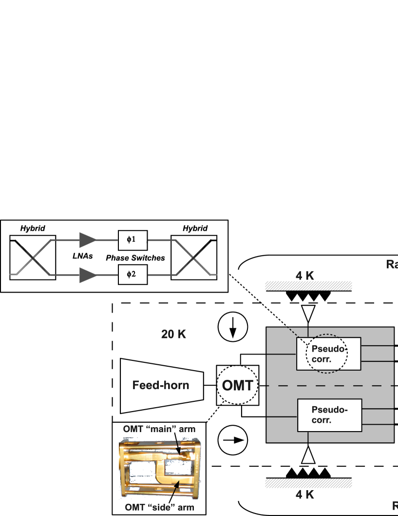
Figure 2: A complete RCA from feed-horn to analog voltage output. The insets show the OMT, the details of the 20 K pseudo-correlator and of the back-end radio-frequency amplification, low-pass filtering, detection and DC amplification.

After detection, an analog circuit in the DAE box removes a programmable offset in order to obtain a nearly null DC output voltage and a programmable gain is applied to increase the signal dynamics and optimally exploit the analogue-to-digital converters (ADC) input range. After the ADC, data are digitally downsampled, requantised and compressed in the radiometer electronics box assembly (REBA) according to a scheme described in [13, 14] before preparing telemetry packets. On ground, telemetry packets are converted to sky and reference load time ordered data after calibrating the analogue digital units (ADU) samples into volt considering the applied offset and gain factors.

To first order, the mean differential power output for each of the four receiver diodes can be written as follows [15, 16, 10]:

$$P_{\rm out}^{\rm diode}=a\,G_{\rm tot}\,k\,\beta\left[T_{\rm sky}+T_{\rm noise}-r\left(T_{\rm ref}+T_{\rm noise}\right)\right],$$ (1)

where $G_{\rm tot}$ is the total gain, $k$ is the Boltzmann constant, $\beta$ the receiver bandwidth and $a$ is the diode constant. $T_{\rm sky}$ and $T_{\rm ref}$ are the average sky and reference load antenna temperatures at the inputs of the first hybrid and $T_{\rm noise}$ is the receiver noise temperature. The gain modulation factor [16, 17], $r$, is defined by:

$$r=\frac{T_{\rm sky}+T_{\rm noise}}{T_{\rm ref}+T_{\rm noise}},$$ (2)

and is used to balance (in software) the temperature offset between the sky and reference load signals and minimise the residual 1/$f$ noise in the differential datastream. This parameter is calculated from the average uncalibrated total power data using the relationship:

$$r=\langle V_{\rm sky}\rangle/\langle V_{\rm ref}\rangle,$$ (3)

where $<V_{\rm sky}>$ and $<V_{\rm ref}>$ are the average sky and reference voltages calculated in a defined time range. The white noise spectral density at the output of each diode is essentially independent from the reference-load absolute temperature and is given by:

$$\Delta T_{0}^{\rm diode}=\frac{2\,(T_{\rm sky}+T_{\rm noise})}{\sqrt{\beta}}.$$ (4)

2.2 Phase switches commanding and configuration

In Figure 3 we show a close-up of the two front end modules of an RCA with the four phase switches which are labelled according to the LNA they are coupled to (M1, M2, S1, S2). Each phase switch is characterised by two states: state 0 (no phase shift applied to the incoming wave) and state 1 (180^∘ phase shift applied) and can either stay fixed in a state or switch at 4 kHz between the two states.

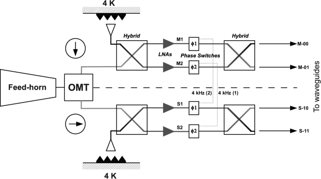
Figure 3: Close-up of the two FEMs of an RCA. There are four phase switches, each one can be fixed in one of its two positions (labelled as 0, 1) or switch at 4 kHz between 0 and 1. Phase switches are clocked and biased by the DAE in pairs (see text and Table 17 for further explanation).

Phase switches are clocked and biased by the DAE and their configuration can be programmed via telecommand. In order to simplify the instrument electronics, phase switches are configured and operated in pairs: by convention they are labelled A/C and B/D. This means that if phase switches A/C are switching at 4 kHz then B/D are fixed both in the same state (either 0 or 1). This simplification, required during the design phase to comply with mass and power budgets, comes at the price of loosing some setup redundancy.

The correspondance between the phase switch labels (A/C, B/D) and the corresponding LNA names (M1, M2, S1, S2), and, as a consequence, the back end module (BEM) output diodes (M-00, M-01, S-10, S-11) is not the same for all RCAs. For the details the interested reader can refer to Table 17 in Appendix E.

3 Overview of Planck-LFI test campaign

During its development, the LFI flight model was calibrated and tested at various integration levels from sub-systems [18, 19, 20] to individual integrated receivers [21] and the whole receiver array [22]. In every campaign we performed tests according to the following classification:

• Functionality tests, performed to verify the instrument functionality.

• Tuning tests, to tune radiometer parameters (biases, DC electronics gain and offset, digital quantisation and compression) for optimal performance in flight-like thermal conditions.

• Basic calibration and noise performance tests, to characterise instrument performance (photometric calibration, isolation, linearity, noise and stability) in tuned conditions.

• Susceptibility tests, to characterise instrument susceptibility to thermal and electrical variations.

Where possible, the same tests were repeated in several test campaigns, in order to ensure enough redundancy and confidence in the instrument behaviour repeatability. A critical comparison, that is central to the subject of this work, is the one between the results of on-ground and in-flight test campaigns. A matrix showing the instrument parameters measured in the various test campaigns is provided in Table 1 of [22]. In the next sections we briefly summarise the on-ground test activities and then provide an overview of the tests carried out during CPV.

3.1 Ground tests

The ground test campaign was developed in three main phases: cryogenic tests on the individual RCAs, cryogenic tests on the integrated receiver array (the so-called radiometer array assembly, RAA) and system-level tests after the integration of the LFI and HFI instruments onto the satellite. The first two phases were carried out at the Thales Alenia Space - Italia laboratories located in Vimodrone (Milano, Italy), system level tests were conducted in a dedicated cryofacility at the Centre Spatiale de Liége (CSL) located in Liége (Belgium).

In Table 1 we list the temperature of the main cold thermal stages during ground tests compared to in-flight nominal values. These values show that system-level tests were conducted in conditions that were as much as possible flight-representative, while results obtained during RCA and RAA tests needed to be extrapolated to flight conditions to allow comparison. Details about the RCA test campaign are discussed in [21] while the RAA tests and the extrapolation methods are presented in [22].

Table 1: Temperatures of the main cold stages during the various ground test campaigns compared to in-flight nominal values.

Temperature	Nominal	RCA tests	RAA tests	System-level
Sky	$\sim 3$ K	$\gtrsim 8$ K	$\gtrsim 18.5$ K	$\sim 4$ K
Ref. load	$\sim 4.5$ K	$\gtrsim 8$ K	$\gtrsim 18.5$ K	$\sim 4.5$ K
Front-end unit	$\sim 20$ K	$\sim 20$ K	$\sim 26$ K	$\sim 20$ K

Cryogenic system-level tests were split into three parts:

• Thermal balance, to validate the overall thermal mathematical model. The ground vacuum test equipment simulated the space environment.

• System cryogenic test, to check and optimise the satellite and instrument performance working at nominal temperatures.

• Thermal cycling test, to check the reliability of all electronics equipment and instruments to temperature variations.

During the various test campaigns the instrument was switched off and moved several times in a time period of about three years. A series of functional tests were always repeated at each location and also in flight, in order to verify the instrument functionality and the response repeatability. No failures or major problems have been identified due to transport and integration procedures.

3.2 In-flight calibration, performance and verification

The Planck cryo-chain [23] is composed by three coolers: a 20 K Hydrogen sorption cooler, passively pre-cooled by the 3^rd V-groove radiator, cools the LFI focal plane and pre-cools the HFI 4 K cooler; a Stirling 4 K cooler that cools the HFI box and feed-horns and provides a 4 K blackbody reference signal to the LFI receivers; a 0.1 K dilution cooler, which is pre-cooled by the 4 K cooler and cools the HFI bolometer filters to $\sim$1.6 K and the HFI bolometer detectors to $\sim$0.1 K. The cooldown of the HFI 4 K stage, in particular, was key during CPV for the LFI as it provided a variable input signal that was exploited during bias tuning (see Section 4.2.2).

The LFI CPV started on June, 4^th 2009 and lasted until August, 12^th when Planck started scanning the sky in nominal mode. At the onset of CPV, the active cooling started when the radiating surfaces on the payload module reached their working temperatures ($\sim$50 K on the 3^rd V-groove, and $\sim$40 K on the reflectors) by passive cooling. This was achieved during the transfer phase. Nominal temperatures were achieved on July, 3^rd 2009, when the dilution cooler temperature reached 0.1 K [24, 23] (see Figure 4).

The CPV was carried out in four phases (see Table 2 for a summary of the overall CPV test campaign): (i) LFI switch on and basic functionality verification, (ii) tuning of front-end biases and back-end electronics, (iii) preliminary calibration tests and (iv) thermal tests.

• LFI switch on and basic functionality tests aimed at verifying functionality either of warm (DAE and REBA) and cold electronics. Functionality tests were performed just after the switch on and periodically during CPV to verify the correct instrument behaviour.

• Tuning tests were performed after the first functional tests to find and set the instrument parameters for optimal scientific performance. Front-end unit biases were tuned exploiting the varying input signal provided by the cooldown of the 4 K cooler to calculate noise temperature and isolation for a large set of bias voltages. Afterwards, the DAE gain and offset parameters were tuned to optimise the DC voltage output at the ADC input range. Finally, optimal REBA parameters were sought to find the best trade-off between telemetry allocation and noise resolution in quantised data.

• Calibration tests provided a preliminary photometric calibration using the CMB dipole and an estimate of the main scientific instrument performance (white noise sensitivity, $1/f$ noise).

• Thermal tests were carried out to characterize thermal and radiometric transfer functions that couple the radiometric response to temperature variation at different locations in the focal plane. This was done by acquiring scientific and housekeeping data with the sorption cooler temperature stabilisation assembly (TSA) turned off in order to increase the level of temperature fluctuations and amplify the effect.

Table 2: List of CPV tests with objectives and references to relevant paper sections

Phase	Test	Objective	Ref.
LFI switch on	Switch on	Verify functionality of electronics units	4.1.1
Functionality	CRYO--01	Switch on LFI front-end unit (FEU) and verify basic	4.1.1
		functionality of all front-end components
	CRYO--02	Verify effectiveness of pseudo-correlation in reducing	4.1.1
		$1/f$ noise
	Spike tests	Characterise 1 Hz spurious spikes	4.1.2
	Drain current test	Characterise LNAs I–V response	4.1.3
	Reference test	Set a functionality reference point	4.1.5
Tuning	Stability check	Verify instrument response stability prior to hypermatrix	4.1.4
	Pre-tuning	Constrain LNA bias space prior to hypermatrix tuning	4.2.2
	Phase switch tuning	Tune phase switch currents for optimal balance	4.2.1
	Hypermatrix tuning	Find the optimal LNA bias configuration by exploring	4.2.2
		the bias space $[V_{\rm g1}^{\rm LNA_{1}},V_{\rm g2}^{\rm LNA_{2}},V_{\rm g1}^{\rm LNA_{1}},V_{\rm g2}^{\rm LNA_{2}}]$.
		The bias space defined during pre-tuning is scanned 4
		times at different temperatures of the 4 K stage.
		For each bias quadruplet noise temperature and
		isolation are calculated
	Tuning verification	Verify optimal biases obtained from hypermatrix tuning	4.2.3
	DAE tuning	Optimise DC voltage output from each detector to the	4.3.1
		ADC input
	REBA tuning	Optimise digital quantisation and compression	4.3.2
Calibration	Noise properties	Preliminary assessment of noise performance and	4.4
		photometric calibration
Thermal	Dyn. thermal model	Assess FPU thermal damping	4.5
	Susceptibility	Assess radiometric thermal transfer functions	4.5

The need for stability over long periods is a key aspect of the Planck surveys and may affect how the instruments are tuned and operated. The large and varied number of activities during most of CPV did not allow to achieve survey-like stability in routine conditions. The first light survey was a period of 15 days at the end of CPV, from August 12^th to August 26^th 2009, where such stability could be achieved and constituted the transition from CPV into Routine phase. In this paper we will not discuss the first light survey.

3.3 CPV Operations

Since the start of Planck operations, during the daily tele-communication period (DTCP) the satellite is in contact with the ground station, operations are implemented and data can be analysed in “realtime” directly at the ESA mission operation centre (MOC). During the CPV, DTCP nominal duration was 5 hours during which telecommand stacks were loaded for test activities that were carried on out of visibility (“timeline” mode). Data were retrieved at the beginning of the following DTCP and arrived at the instrument data processing centre about 5 hours later.

LFI switch-on and the first functional tests (CRYO-01, CRYO-02 and drain current verification, see Section 4.1) were performed in real-time in order to promptly monitor the instrument behaviour and stop the procedure in case of contingency. Although few additional short tests (e.g., REBA tuning) were added in realtime to speed up data analysis approach, the bulk of the CPV tests were carried out in timeline mode.

During the CPV, Planck scanned the sky at 1 revolution per minute repointing the spin axis by 1^∘ each day: this way it was possible to efficiently integrate and remove the sky signal, which facilitates noise analysis. Moreover several tests were run before digital quantisation and compression optimisation. In these cases data were acquired unquantised and uncompressed with a sampling rate reduced to 16 Hz for all channels in order to fit within the allocated telemetry bandwidth. At the end of CPV, Planck entered its nominal scanning strategy and data acquisition mode which has been maintained throughout the subsequent operations.

4 In-flight testing of Planck-LFI

4.1 Functionality tests

In this section we discuss the set of functional tests that were run immediately at switch on and several times during CPV when the instrument changed thermal configuration (see Figure 4). Their main objectives were:

• to verify communication between the analogue and digital electronics and between the instrument and the satellite,

• to check the electrical connection between the power supply units and the receiver active components (LNAs and phase switches),

• to verify the functionality of the receiver active components,

• to assess the instrument stability in terms of voltage output and drain current,

• to measure the radiometer characteristic curves (drain current vs. voltage output) and compare them with ground measurements.

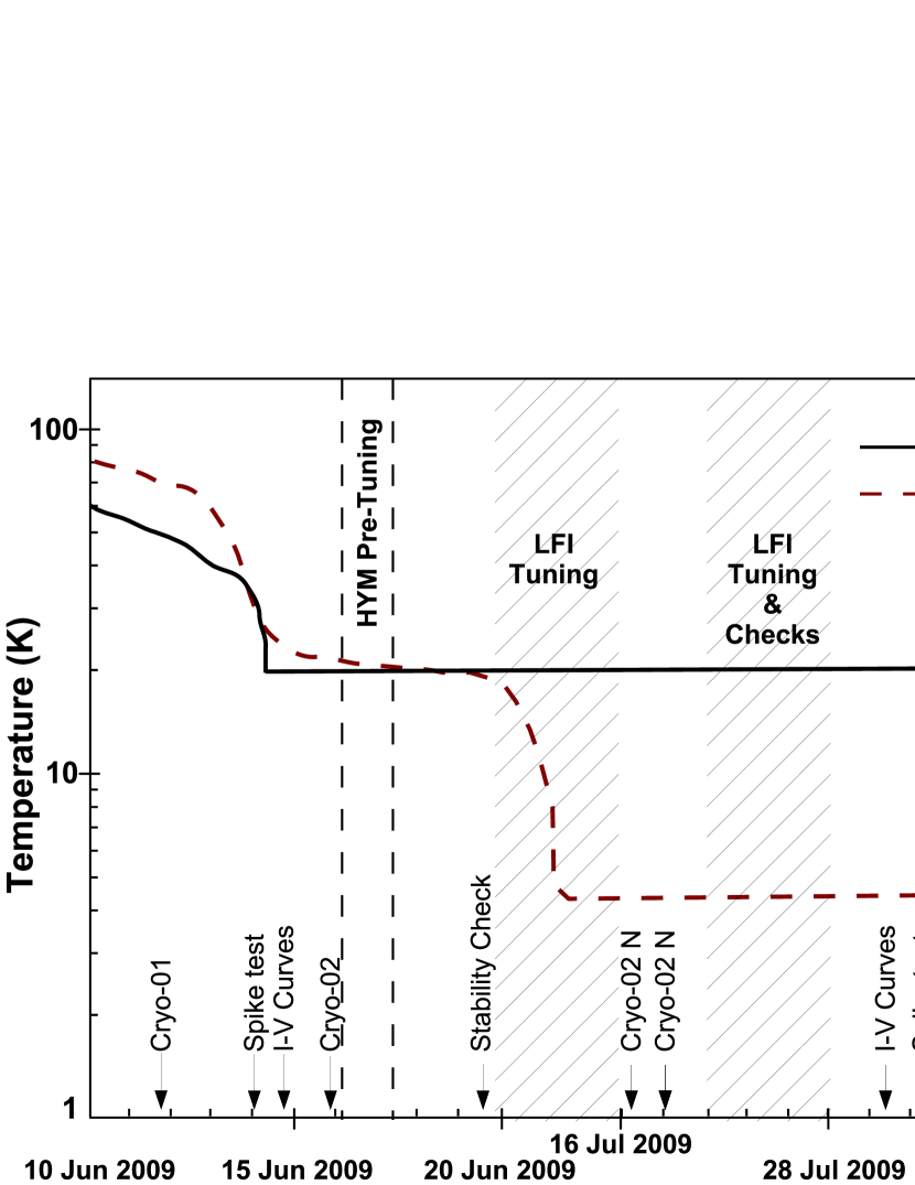
Figure 4: Functional tests performed during CPV; the 4 K stage and the FPU Temperature are superimposed.

4.1.1 LFI switch on and basic functionality

The LFI was switched on June, 4^th 2009. The procedure was carried out in two steps: during the first step the REBA was switched on and commissioned by verifying memory contents of its units (the Science and Data Processing Units), loading and starting the application software, and finally synchronising the REBA with spacecraft on board time. During the second step, the DAE was switched on and commissioned by verifying its main functionalities, synchronising the DAE clock with the spacecraft on board time, verifying its memory contents, and finally starting scientific data processing. At the end of this phase the LFI back-end unit was fully on.

After commissioning, the LFI front-end modules were gradually biased, powering the LNAs and the corresponding phase switches one by one (CRYO-01 test). The bias configurations were the same used on ground apart from LFI18M1 and LFI27M1, that were biased with a lower drain voltage to reduce the risk of ADC saturation, and LFI24M1, for which the voltage was slightly changed to avoid oscillations that were occasionally observed during ground tests. The sequence was chosen in order to minimise the electric cross-talk due to the common return resistance in the cryo harness (see Table 13, Appendix A). The functionality was verified by checking that during the procedure the voltage output from each detector followed the expected pattern due to the sequential switching on of the FEM components. The details of the various steps are reported in Appendix B, Table 16, while the typical pattern followed is sketched in Figure 5.

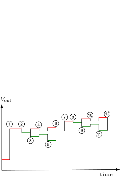
Figure 5: Expected voltage output pattern during the CRYO-1 test, numbers correspond to the same reported Appendix B in Table 16. Red and green lines represent data labelled as “sky” or “reference load” samples. Steps showing just one line refer to the ‘4 kHz disabled’ condition.

We also compared the drain current measured in the various steps with the corresponding values measured on ground (see Figure 6). Although the focal plane temperature was different in the two cases (in the range [38.5 K-35.8 K] during CRYO-01 performed on ground and in the range [36.1 K- 20 K] during the same in-flight test) drain current measurements were repeatable within 10% in all cases, besides those channels for which the switch-on bias voltages was changed (LFI24M1, LFI27M1, LFI18M1).

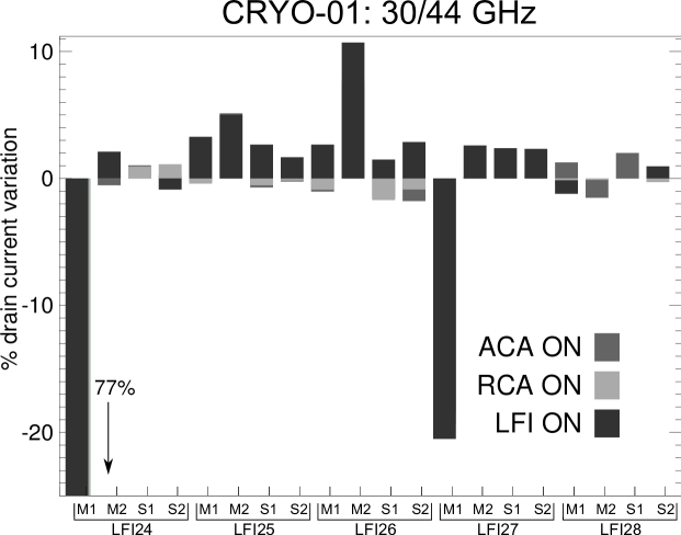
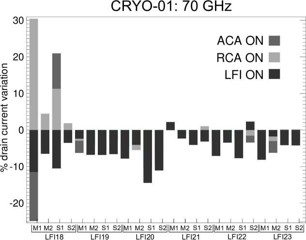
Figure 6: Comparison of drain currents measured during on-ground and in-flight CRYO-1 tests. The percentage variation is defined by $(I_{\rm drain}^{\mathrm{flight}}-I_{\rm drain}^{\mathrm{ground}})/I_{\rm drain}^{\mathrm{ground}}$. The relative drain current variation is displayed for three different configurations: one amplifiers chain assembly (ACA) on, one RCA on, the whole LFI on. For each channel, the three data sets are stacked with different colors on the same bar. When the differences between the three steps are negligible, just one color is displayed.

After all the channels were nominally biased, we assessed instrument functionality and the effectiveness of the pseudo-correlation differential scheme in reducing 1/$f$ noise instabilities. To achieve this we checked that:

• drain currents were comparable with those measured during ground tests ($\pm$5%);

• 1/$f$ noise knee frequency, $f_{\rm knee}$, was reduced to less than $\sim$1 Hz after sky-reference load differencing.

The CRYO-02 test consisted of a two-hours data acquisition split into four 30-minute steps in which the radiometers were operated in switching mode testing all the four possible phase switch configurations in series (see Table 3).

Table 3: The four CRYO-02 steps with the corresponding phase switch configurations; “sw.” indicates the 4 kHz switching.

Step n.	A/C	B/D
1	sw.	0
2	sw.	1
3	0	sw.
4	1	sw.

In Figure 7 we show a comparison of drain currents measured in-flight and on-ground CRYO-02 test for the four phase switch configurations. Results show that all the drain currents have been found reproducible within $\pm$2% apart from LFI26M2 for which we recorded a 8.6% ($\sim$1 mA) higher drain current compared to ground measurements. Although the reason of this discrepancy has not been understood the LNA showed full functionality as proved by the drain current verification test (Section 4.1.3).

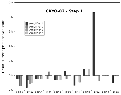
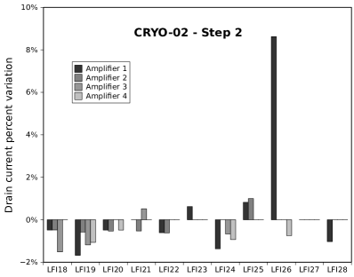
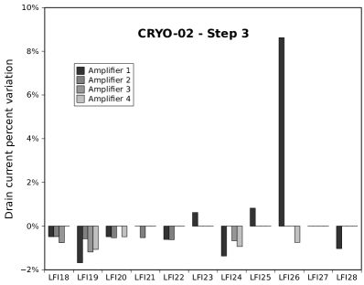
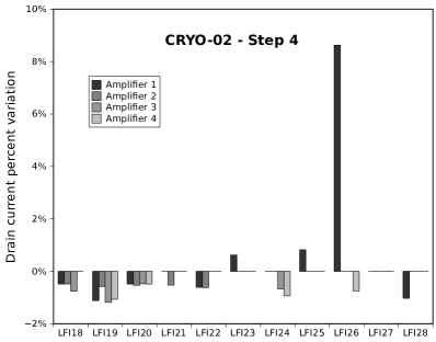
Figure 7: Comparison of drain currents measured during CRYO-02 tests performed in-flight and on-ground. The percentage variation is defined by $(I_{\rm drain}^{\mathrm{flight}}-I_{\rm drain}^{\mathrm{ground}})/I_{\rm drain}^{\mathrm{ground}}$. No bars are displayed when the drain current variation was less than $0.1$ mA

Figure 8 summarises the calculated knee frequency for all 44 channels during the CRYO-02 test for all the tested phase switch configurations. The knee frequency was essentially independent from the switch configuration and less than 1 Hz for all channels apart from the following cases:

• LFI23M-00 and LFI23M-01 with B/D switching (steps 3 and 4),

• LFI21S-11 and LFI24S-11 with B/D switching and A/C set to 0 (step 3).

We now discuss these two cases separately.

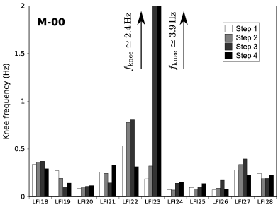
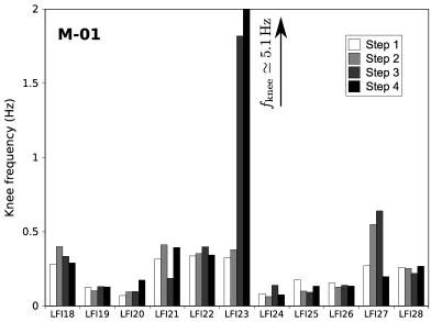
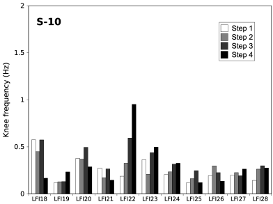
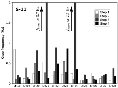
Figure 8: Knee frequencies of differenced data measured during the CRYO-02 test. For all channels apart from LFI23M-00, LFI23M-01, LFI21S-11, LFI24S-11 knee frequencies were less than 1 Hz and comparable in the four states of the phase switches.

High knee frequency in LFI23M-00 and LFI23M-01

In Figure 9 we show the power spectral densities (PSDs) of differenced data streams from the LFI23M-00 detector during the four steps of the CRYO-02 test. The plots on the left indicate a nominal behaviour: a white noise plateau at high frequencies and a 1/$f$ tail below that does not prevent to detect the sky signal visible as a spike at 16 mHz, the satellite spin frequency. The plots on the right, instead, (corresponding to steps 3 and 4, i.e. with B/D switching) indicate an anomalous behaviour: there is no white noise plateau and the spike at 16 mHz caused by the sky signal (CMB dipole and galaxy) is not visible. The noise spectrum, in this case, was dominated by 1/$f$ noise. PSDs of LFI23M-01 show the same trend and are not reported here for simplicity.

This anomaly was not new as was detected for the first time during the satellite ground tests and was confirmed in flight. The root cause of this extra noise was not fully understood but the anomaly could be avoided by keeping the LFI23 RCA in the A/C switching configuration at the price of redundancy loss for the phase switch configurations of this RCA.

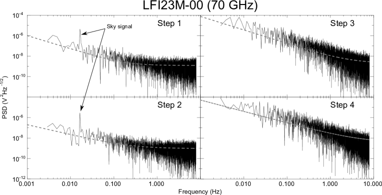
Figure 9: PSD of differenced data from LFI23M-00 detector during the CRYO-02 test. The spike around 16 mHz in the the two panels on the left is determined by the sky signal (CMB dipole and galaxy).

High knee frequency in LFI21S-11 and LFI24S-11

In Figure 10 we show the PSDs of differenced data streams from the LFI21S-11 and LFI24S-11 during the four steps of the CRYO-02 test. In these two cases the four spectra are essentially comparable. The high numerical value calculated for $f_{\rm knee}$ did not indicate, in this case, a real anomaly in the phase switch configuration.

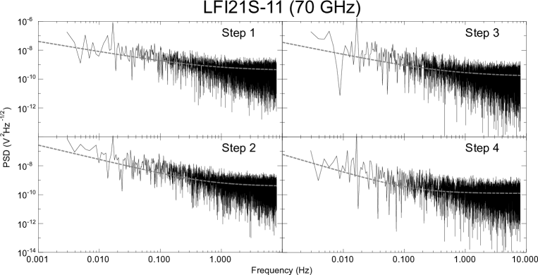
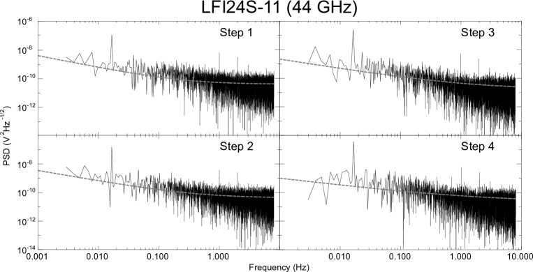
Figure 10: PSD of differenced data from LFI21S-11 and LFI24S-11 detectors during the CRYO-02 test. The behaviour was nominal in all the tested configurations.

4.1.2 Spurious 1 Hz spikes

During instrument ground tests [25, 22] an artifact was identified in the LFI data which is characterised as a set of extremely narrow spikes at 1 Hz and higher harmonics. These artifacts are nearly identical in sky and reference samples, and are almost completely removed by the LFI differencing scheme. Extensive testing and analysis identified the spikes as a disturbance on the science channels from the housekeeping data acquisition, which is performed by the DAE at 1 Hz sampling. An example is given in Figure 11.

Frequency spikes in scientific data have been checked several times during ground and flight tests to verify their stability and their impact on the radiometric data. The test consisted in data acquisitions in several radiometer configurations:

• Radiometers unbiased. In this case only the warm electronics noise was acquired. This was the most favourable condition to measure the spike amplitudes.

• Front-end modules unbiased and back-end modules in nominal bias conditions.

• All instrument in nominal bias conditions. In this case the data acquisition was repeated for all phase switch configurations to check for possible phase switch interactions.

Here we summarise results obtained in the first configuration, used to characterise spike stability, and in the third configuration, that highlights the impact of frequency spikes on nominal science data.

In Appendix C (Figure 49) we show the amplitude spectral density of 1 Hz frequency spikes in all the LFI outputs measured during ground and flight tests with radiometers completely unbiased. These results show that the spike amplitude was very stable and reproducible among the various test campaigns. Two particular features can be noticed around 3.5 Hz and 12.5 Hz in the LFI22M-00 and LFI22M-01 plots. These correspond to two broad spikes that were detected in the electronics noise output of these two channels independently from the status of the housekeeping sequencer. Their cause is presently unknown. A detailed view of these frequency spikes is provided in Figure 12.

Figure 11: Amplitude spectral density (ASD) of data from the LFI18M-00 science channel with the housekeeping sequencer on (left panel) and off (right panel). In this test the radiometers were unbiased so that only the noise of the warm electronics was recorded. Spurious 1 Hz spikes clearly disappeared when the housekeeping acquisition was turned off.

Figure 12: ASD of data from the LFI22M-00 and LFI22M-01 science channels with the housekeeping sequencer off. Two broad spikes are present at frequencies of about 3 Hz and 12 Hz. These spikes do not depend on the status of the housekeeping sequencer and their cause is presently unknown. Also in this case the radiometers were unbiased.

Although spikes are below noise level in frequency domain, it was possible to obtain a template of the spurious signature in time domain exploiting its synchronous characteristics and binning several days of data in 1-second time windows. These templates have then been used to correct the 44 GHz data, which are the more affected by this effect. Details of the spike removal pipeline are provided in [17] while the assessment of the residual on the scientific results is discussed in [8].

4.1.3 Drain current verification

The receiver response to front-end bias changes was checked several times by means of the so-called drain current test. During this test the two gate voltages, $V_{\rm g1}$ and $V_{\rm g2}$, were changed independently for each front-end LNA spanning a pre-defined set of values and, for each value, the average drain current was recorded. The signal unbalance between the sky (at $\sim 3$ K) and the reference load (at $\gtrsim 20$ K) temperatures was exploited to estimate the noise temperature according to the formula (“Y–factor method”):

$$T_{\rm noise}=\frac{T_{\rm ref}-T_{\rm sky}}{Y-1},\,\mbox{with }\,Y=\frac{V_{\rm ref}}{V_{\rm sky}}.$$ (5)

The channels were grouped in pairs in order to minimise electric cross-talks caused by the cryo harness common ground return (see Appendix A, Table 14). Two channels were tested at a time, all the other channels were kept to their default bias values. During CPV the drain current test was run three times: (i) before the bias pre-tuning (see Section 4.2.2) to compare the response with on-ground test results, (ii) after the bias tuning phase (see Section 4.2.2), to check for any changes that could have been induced by the several bias changes occurred during tuning, and (iii) at the very end of the tuning activities when new default biases were implemented.

In Figure 13, we show an example of the test results obtained for the channel LFI26M1 during the first run. The top panels show drain currents as a function of the two input gate bias voltages, while the bottom panels show noise temperature variations as a function of $V_{\rm g1}$ and $V_{\rm g2}$. Figure 13 shows an excellent match between ground and flight measurements providing a further verification of the functionality of front-end LNAs after launch and cooldown.

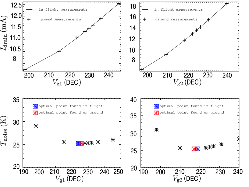
Figure 13: Example of drain current test results for channel LFI26M1. Top panels: drain currents (line for flight and crosses for ground data), bottom panels: noise temperatures measured in-flight, as a function of the input bias voltages. Minimum noise temperatures are highlighted in blue and red respectively. Note that the bias units are DEC units that are used to set the voltage in the DAE: see Table 4 for a rough conversion into physical units.

Notice that gate voltages are displayed using the adimensional code (from 0 to 255) used to set the voltage in the DAE rather than the voltage in physical units. The reason is that the actual voltage reaching the FEMs depends on the harness resistive drop which depends on the satellite thermal configuration. The DAE code, therefore, was the most robust way to refer to the LNA bias voltages. The interested reader can roughly convert the DAE code into the actual delivered voltage (neglecting the harness resistance drop) using a linear calibration with the values detailed in Table 4. It is important to underline that the calibration table actually used to convert DAE codes to physical units is channel dependent, but it is not provided here for simplicity.

Table 4: Values for a zero-order calibration of DAE bias codes into physical units.

	DAE code = 0			DAE code = 255
	$V_{\rm drain}$	$V_{\rm g1}$	$V_{\rm g2}$	$V_{\rm drain}$	$V_{\rm g1}$	$V_{\rm g2}$
30 GHz	0.0 V	-4.0 V	-4.0 V	1.4 V	2.0 V	2.0 V
44 GHz	0.0 V	-4.0 V	-4.0 V	1.4 V	2.0 V	2.0 V
70 GHz	0.0 V	0.0 V	0.0 V	1.0 V	2.0 V	2.0 V

In Figure 14, we show a comparison of results coming from the same test at system level in CSL and during the CPV runs first and third, for different channels. To facilitate the comparison, the 1^st run and CSL curves were offset on the Y-axis as reported on the label (CPV1-CSL and CPV3-CPV1). In most cases the matching is very good, despite the different bias defaults; in a few cases, mostly corresponding to channels characterized by a large difference in their bias setup in the two frames, or in the bias setup of other channels belonging to the same power group, we found larger differences. Plots for all channels are given in Appendix D.

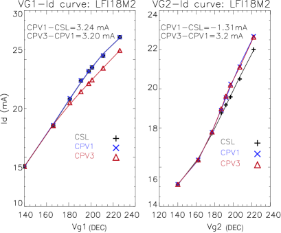
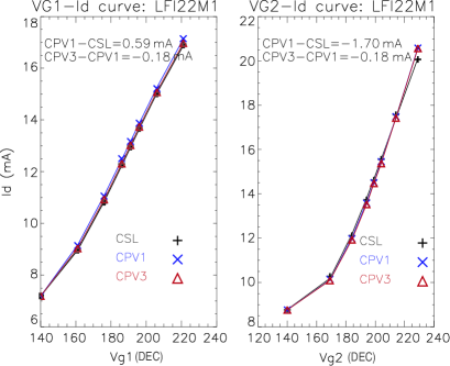
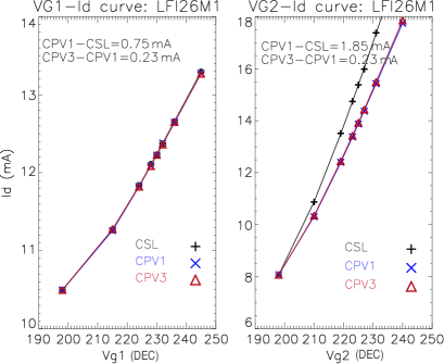
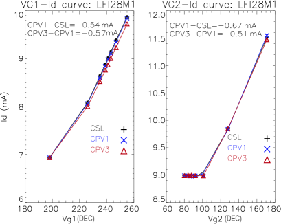
Figure 14: I-V curves: for each channel (LFI18M2, LFI22M1, LFI26M1, LFI28M1) we show two plots representing the drain current behavior respectively versus $V_{\rm g1}$ and $V_{\rm g2}$. Black crosses refer to results from CSL system level tests, red triangles to the 3^rd one, blue crosses to 1^st run; solid lines represents the corresponding polinomial fits. Curves are offset to facilitate the comparison, the offset amount is reported on the internal labels. Note that the bias units are DEC units that are used to set the voltage in the DAE: see Table 4 for a rough conversion into physical units.

4.1.4 Stability check

During this test the instrument was left undisturbed for 12 hours in nominal, pre-tuned bias configuration, with the objective to verify the instrument readiness for the bias tuning activity. The instrument stability was verified by checking the following observables: (i) drain currents, (ii) output voltages, (iii) knee frequency of differenced data.

It is important to notice that during this test the temperature of the 4 K stage was still around 20 K with no stability optimisation. This resulted in a knee frequency which was much higher than the required 50 mHz for optimal scientific performance. Therefore in this test we checked that the knee frequency calculated from differenced datastreams were much less than those calculated from undifferenced data and, in general, less than $\sim$1 Hz.

In the top and middle panels of Figure 15 we show the percentage variation of (sky) voltage output and drain currents during the stability test. These results show that variations in the sky voltage output were less than 0.2%, with the exception of LFI18M-00 and LFI18M-01 showing a stability of 0.5%, a typical figure for these two channels. Drain currents were stable within 0.1% with three cases slightly exceeding this figure: LFI18M1, LFI21M1 and LFI22S2. The drain current behaviour for these three devices is plotted in Figure 16 compared to the drain current measured for the twin amplifier. The higher unstability level of these three amplifiers was already known since ground tests and has never represented a problem.

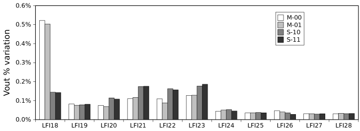
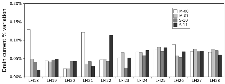
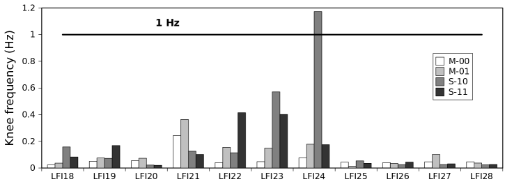
Figure 15: Main stability indicators measured during the stability test. Top panel: sky output voltage % variation. Middle panel: drain current % variation. Bottom panel: $1/f$ knee frequencies of differenced data.

The bottom panel in Figure 15 shows the $1/f$ knee frequency of differenced data for all channels.

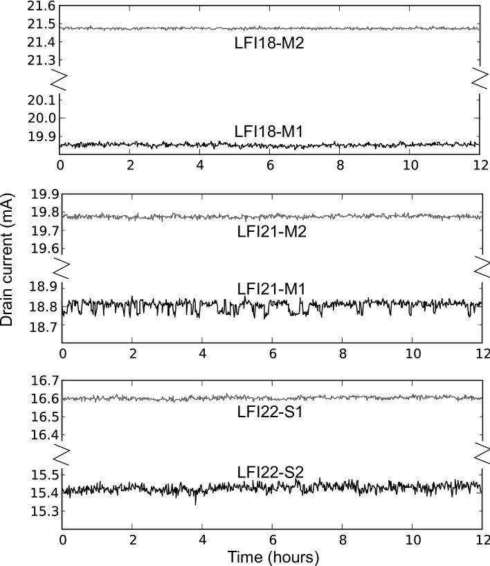
Figure 16: Drain currents during the stability test. Instabilities in LFI18M1, LFI21M1 and LFI22S2 are highlighted by comparison with drain currents from their twin amplifiers.

4.1.5 Reference test

Close to the end of the test Campaign, a functionality assessment was performed with a double objective:

• to verify that no damages, or any other evident changes, were occurred in the radiometers during the test campaign;

• to characterize the LNAs and phase switches response with the LFI in nominal conditions. This test was thought as a tool to check for any possible anomalies in one or several channels during the nominal survey, without disturbing the acquisition of all the other channels.

The test was run in two parts. The first part (RT-1) is identical to the CRYO-02, with radiometers powered with exactly the same CRYO-02 biases but with different thermal boundaries (during the first CRYO-02 the LFI focal plane was almost at its nominal temperature but the 4 K stage was still at about 21 K). The second part (RT-2) followed a procedure very similar to the CRYO-01 (see Appendix B) but with the tuned LNAs biases. The two steps were executed about ten days apart due to scheduling requirements but this did not affect the general result.

The objective of RT-1 was to check the functionality of radiometers in all the possible phase switch and 4 kHz combinations after the hypermatrix tuning: LNAs drain currents and noise properties (1/$f$, white noise, spikes) were compared with those measured during CRYO-02. The sky scientific outputs were compared as well (reference outputs were not compared due to the different thermal conditions of the 4 K stage during the two tests).

A strong drift in the Voltage output characterized the whole test; this was probably due to variation in LNA power dissipation once CRYO-02 biases were set. As during the first CRYO-02, some instabilities were observed in the drain currents of a few radiometers (LFI21S1 and LFI22S2).
Drain current comparison (see Figure 17) with previous CRYO-02 showed the excellent consistency of the two tests: differences are all below 5%, on average below 2% with the exception of LFI18M1, already known for being characterized by a larger instability.
The sky-voltage comparison (Figure 18) confirmed the agreement: differences are below 1% in most cases, around 5% in the remaining confirming the good radiometer isolation.

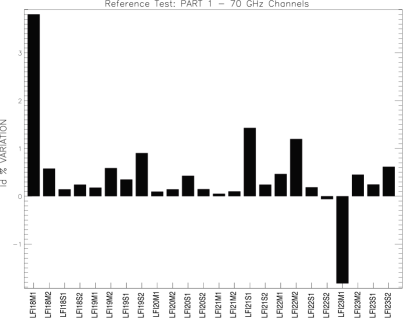
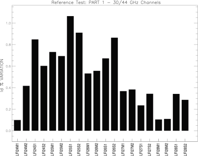
Figure 17: Reference Test Part 1: Drain Current comparison with CRYO-02 data.

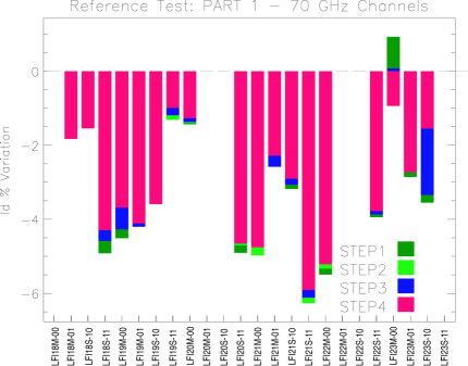
Figure 18: Reference Test Part 1: Output voltage (sky) with CRYO-02 data sets: the four steps are stacked on the same bar for each channel. When differences among the four steps are negligible, just one color is displayed on each bar. For three radiometers (LFI20M-00, LFI20M-01, LFI22M-00, LFI22M-01, LFI23S-10, LFI23S-11) the comparison is missing because of an ADC saturation caused by a wrong settings in the DAE biases.

The second part of the reference test, RT-2, confirmed the full functionality of radiometers as all the devices responded as expected. In detail we checked:

• the functionality of V_g1 and V_g2 amplification stages;

• phase switch diodes ability to exchange signals (sky/ref) when the polarization status is inverted and to separate signals when I₁ or I₂ phase switch bias currents are lowered or increased;

• the 4 kHz switching;

• DAE ability to tag signals (sky/ref) correctly when the P/S status or the switching 4 kHz circuit are inverted;

• the functionality of the Back-End warm LNAs.

This test also provided a quantitative reference point for any comparison during the mission.

4.2 Front-end electronics tuning

4.2.1 Phase switch tuning

The objective of this test was to find the optimal bias currents to the front-end phase switches that balance the wave amplitude in the two phase switch states. Because an optimal balance affects the receiver isolation, the test was performed before the tuning of the front-end modules amplifiers. The test was repeated after the front-end amplifier tuning to show that the optimal phase switch biases were independent from the amplifier bias values. As planned the test was performed only on 30 and 44 GHz RCAs by varying the current supply (I₁ and I₂) in order to reach the optimal balance (this choice was driven by the switch time response that in the 70 GHz devices was longer compared to the 30 and 44 GHz and further increased when the diode currents were lowered: the option to setting phase switch biases to maximum allowed values was preferred to phase balancing [26, 20]). When this condition is reached, the sky-reference output difference is very close as possible to zero when the amplifier in the opposite leg is set to zero bias. In fact, when an ACA is switched off, the output at each diode in the two switch states is (Seiffert et al. 2002 page 1187):

$$V_{\rm even}^{\rm bem}\propto{1\over\sqrt{2}}\sqrt{A_{2}}e^{i\phi_{2}}G_{\rm FEM}\left(N_{\rm FEM}+{S_{\rm sky}+S_{\rm ref}\over\sqrt{2}}\right)$$ (6)

$$V_{\rm odd}^{\rm bem}\propto{1\over\sqrt{2}}\sqrt{A_{1}}e^{i\phi_{1}}G_{\rm FEM}\left(N_{\rm FEM}+{S_{\rm sky}+S_{\rm ref}\over\sqrt{2}}\right),$$ (7)

where ${\phi_{1,2}}$ represent the phase shifts in the two switch states (in LFI baseline ${\phi_{1}}=0$ and ${\phi_{2}}=\pi$); $A_{1,2}$ represent the fraction of the signal amplitudes transmitted after the phase switch in the two switch states (for lossless switches $A_{1,2}=1$); $N_{\rm FEM}$ is the Front-End LNA noise . In the case of a tuned phase switch, the difference between the two voltages of the two states, $\delta$ = $V_{\rm even}^{\rm bem}$-$V_{\rm odd}^{\rm bem}$, is close to 0.

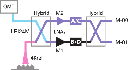
Figure 19: Radiometer scheme showing the phase switch tuning. The figure shows the case of the LFI24M when one amplifier is switched off. Under this condition the output of both hybrid output arms experience the same signal unless the phase switches is not well balanced. Reference and sky signals, disentangled at the 2^nd hybrid output, are expected to be close under balanced conditions. The figure is a shot of a 1/8000 s.

For each pair I₁ and I₂ we measured the following quantities:

• $V_{1}^{\rm even}$ and $V_{1}^{\rm odd}$: average over the time window respectively of the even and odd samples of the signal at first detector;

• $\Delta V_{\rm 1}$: difference at the first detector defined as $\Delta V_{\rm 1}=V_{1}^{\rm even}-V_{1}^{\rm odd}$;

• $V_{2}^{\rm even}$ and $V_{2}^{\rm odd}$: average over the time window respectively of the even and odd samples of the signal at second detector;

• $\Delta V_{\rm 2}$: difference at the second detector defined as $\Delta V_{\rm 2}=V_{2}^{\rm even}-V_{2}^{\rm odd}$;

• $\Delta V$: figure of merit parameter defined as $\Delta V=\sqrt{\Delta V_{1}^{\rm 2}+\Delta V_{2}^{\rm 2}}$.

For each phase switch a matrix of I₁ and I₂ values was applied, the ranges were set on the basis of the ground test results. The matrix approach, already verified on ground [26], was selected as the best option to evaluate the best balance condition for phase switches by computing the minimum value of $\Delta V$. Notice that phase switch currents are displayed using the adimensional code (from 0 to 255) used to set the bias in the DAE rather than the current in physical units. At first order the interested reader can convert the DAE code into the actual delivered current using a linear calibration with the values detailed in Table 5. It is important to underline that the calibration table actually used to convert DAE codes to physical units is channel dependent, but it is not provided here for simplicity.

Table 5: Values for a linear calibration of DAE bias codes into physical units, for all LFI channels.

DAE code = 0	DAE code = 255
I1, I2	I1, I2
0.0 mA	1.0 mA

Two examples of the analysis performed are shown in Figure 20, while the behavior of all the 30 GHz and 44 GHz channels is displayed in Appendix E, Figure 51 in terms of relative percentage balance maps $\delta=100\cdot\Delta V/\left(V_{\rm ave}\right)$, in colored contour plots for the whole set of applied I₁ and I₂ combinations.

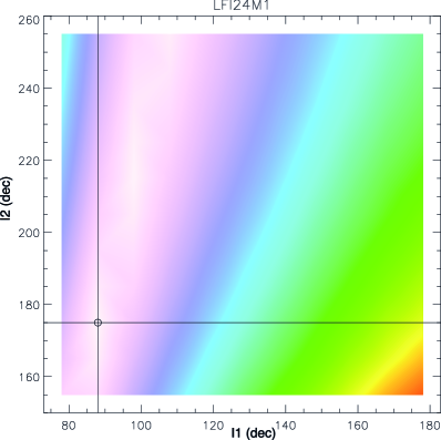
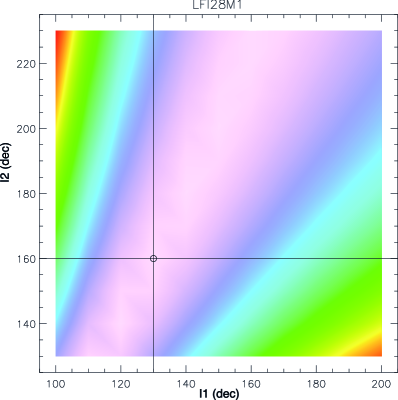
Figure 20: Phase switch tuning maps for the two channels LFI24M1 (left panel) and LFI28M1 (right panel). I₁ bias lies on x-axis, I₂ bias on y-axis. The bright zone identifies small unbalances. The map represents the figure of merit, $\Delta V$, as defined in the text. Note that the bias units are DEC units that are used to set the bias in the DAE: see Table 5 for a conversion into physical units.

Table 18 in Appendix F, reports the values found from the automatic routine, the optimized values and the flight default values applied during the mission. It should be noted that in some cases the best tuning condition was clearly in a region outside the grid scanned with phase switch tuning performed during system level tests in CSL. This is the case of LFI24M1, LFI25M2, LFI25S1, LFI26M1, LFI26S2, LFI27M1, and marginally of LFI24M2, LFI24S2, LFI27M2, LFI27S1, LFI27S2, LFI28S2. Two examples of resampled grids compared to the original regions explored during phase switch tuning at system level are reported in Figure 21.

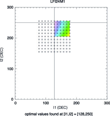
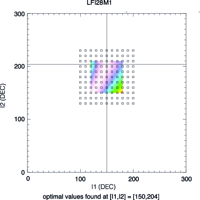
Figure 21: CSL system level tests phase switch tuning maps for the two channels LFI24M1 (left panel) and LFI28M1 (right panel) compared to the bias grid sampled during the same test performed in CPV. I₁ bias lies on x-axis, I₂ bias on y-axis. The bright zone identifies small unbalances. The map represents the figure of merit $\Delta V$ as defined in the text. Open squares represent the points explored during CPV. Note that the bias units are DEC units that are used to set the bias in the DAE: see Table 5 for a conversion into physical units.

The optimal I₁ and I₂ pairs derived automatically from the routine were checked one by one and eventually optimized on the basis of the following criteria:

• Comparison with cryogenic ground tests at CSL [26];

• Balancing of I₁ and I₂ privileging biases providing high phase switch currents (guaranteeing small losses).

According to the last two items, results were hand refined for the following ACAs: LFI24M1, LFI25M2, LFI27M2, LFI27S2, LFI28M2.

Phase switch tuning verification

This test was aimed at verifying that the phase switch tuning results are independent (or marginally dependent) on the bias configuration of the LNAs. In fact the phase switch tuning was performed before the LNAs hypermatrix tuning, with the LNAs in pre-tuned conditions (with ground test CPV biases). The phase switch tuning verification was instead run after the hypermatrix tuning, with the LNAs in “Tuned conditions”.
However two events during the test compromised the result: an electric oscillation occurred in the RCA24 (caused by an error in the soft switch-on procedure) and the signal saturation on the RCA27 (caused by a wrong bias set at DAE level, amplifying the signal outside the allowed range). Because of these, the full purpose of this test was not reached. Actually, even if at first order the phase switch tuning test results were confirmed, any second order effects due to the phase switch interaction with the different LNAs bias remained unexplored.

4.2.2 LNAs tuning

Optimal front-end biases were determined during CPV by exploring a large set of voltage values and assessing, for each of them, the radiometer performance in terms of noise temperature and isolation. Tuning was performed in two phases: a pre-tuning phase to constrain the bias space around best-performance regions and a proper tuning phase during which the bias regions identified during pre-tuning were finely sampled in order to converge towards the optimal values.

During both phases the bias space was sampled according to a so-called hypermatrix (HYM) strategy in which several bias quadruplets, $[(V_{\rm g1},V_{\rm g2})_{\rm LNA-1},(V_{\rm g1},V_{\rm g2})_{\rm LNA-2}]$, were varied simultaneously for each radiometer. This strategy increased the sampled parameter space with respect to ground tuning tests [26], where the bias space was sampled independently for the two ACAs over a two-dimensional space.

In both phases the test was performed simultaneously on several RCAs which were grouped according to a scheme that minimised the bias cross talk effects along the harness lines. The details of the grouping scheme are reported in Appendix A, Table 15. ACAs not under test were set at their default biases (CSL biases) with the only exception of the phase switch biases that during the proper tuning phase were set to the optimal values resulting from the phase switch tuning (see Section 4.2.1).

A dedicated code was developed to analyse the tuning data and navigate the four-dimensional bias space. Data display was performed using the concept of condensed bias maps of radiometer noise temperatures, isolation and drain currents: see Figure 22 for a few examples. These are contour plots in the $V_{\rm g1},V_{\rm g2}$ space for the LNAs of a given radiometer. Each point in the plot is the average of the best 20% noise temperature values determined by the quadruplets sharing that particular $V_{\rm g1},V_{\rm g2}$ pair. The interface allows to show, for each point, the quadruplet yielding best performance among all the possible combinations. The same approach was used to map isolation and drain currents.

Hypermatrix analysis was further refined by applying a non linear model of detector response [27] and other corrections accounting for gain variations due to thermal instabilities along the four steps (see 4.2.2 section). As expected, with respect to the standard approach, the hypermatrix method did not produce major changes in mapping the optimal quadruplets.

At the end of the proper tuning, a verification test (see Section 4.2.3) was performed to directly calculate the white noise for each bias quadruplet. Probably due to the too short integration time, the power of this test was weaker than expected: despite of the overall consistency with the HYM tuning results, this test was not able to provide any extra improvement to the bias optimization process.

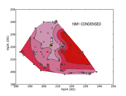
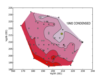
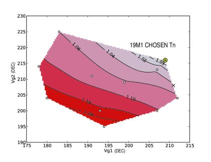
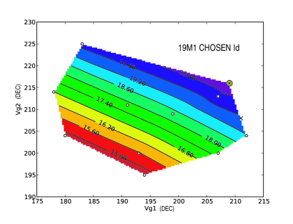
Figure 22: Condensed bias maps for LFI19M as a function of $V_{\rm g1}$, on x-axis, and $V_{\rm g2}$, on y-axis. Top panels, noise temperature maps: each point represents the condensed properties of bias quadruplets in the bias space of the M1 amplifier (left panel) and of the M2 amplifier (right panel). Colour scale ranges from red (highest noise temperatures) to light-grey (lowest noise temperatures), normalized to the lowest noise temperature. Yellow circles correspond to the optimal bias quadruplets. Crosses correspond to results from CSL system level tests. Contours represents level of constant noise temperature. Bottom panels: noise temperature map obtained when the M1 bias corresponding to the best condensed noise temperature are fixed (left panel), the colour scale and contour meaning is the same as for the top panels; drain current map corresponding to the noise temperature map shown on the left (right panel), the colour map, from red to blue, represents increasing drain current values, contours represents level of constant drain current. Refer to the text for further explanations.

Pre-tuning.

The aim of this first phase was to determine, for each radiometer, a relatively small bias region where best performance was expected. Pre-tuning was performed by scanning a large bias volume determined using results from ground tests combined with a drain current model applied to predict the expected drain current for each bias configuration. This test lasted 27 hours.

During the test the temperature of the 4 K cooler was still above 20 K and we exploited the large unbalance between the sky and reference load signal to estimate the noise temperature for each diode according to the equation:

$$T_{\rm noise}=\frac{T_{\rm ref}-Y^{\rm*}\cdot T_{\rm sky}}{Y^{\rm*}-1},$$ (8)

where $Y^{\rm*}=V_{\rm ref}/V_{\rm sky}$, and $V_{\rm sky}$ and $V_{\rm ref}$ are the sky and reference load voltage outputs measured by each diode thanks to the 4 kHz phase switch. This is a modification of the standard approach based on the Y–factor (see Section 5) calculated on the temperature variations of the target load between two values high and low [26]. Although pre-tuning scheme intrinsically prevented to calculate isolation, we measured drain currents to assess the gain balance of each amplifier pair in order to exclude bias voltage configurations leading to a too large drain current imbalance.

The integration time for each bias was a compromise between the test duration constraints and the necessary relaxation time after each bias change. We chose 15 seconds for the 70 GHz channels and 9 seconds for 30 and 44 GHz channels which relax faster (see Figure 23). For each bias step, only the last three seconds of data were effectively used in the analysis.

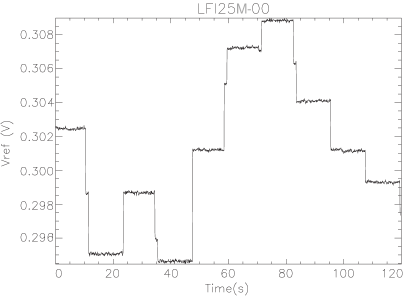
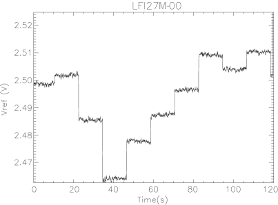
Figure 23: Three examples of the voltage output step caused by a bias change. Top panel: LFI19M-00, bottom panels: LFI25M-00 (left), LFI27M-00 (right). Each panel covers a time window of 120 seconds. Voltage outputs of 30 and 44 GHz channels relaxed faster than 70 GHz channels. In all cases only the last three seconds of data were used in the analysis.

The accuracy in the noise temperature measurements depends on the levels and stability of sky and reference load signals ($T_{\rm sky},T_{\rm ref},\sigma_{T_{\rm sky}},\sigma_{T_{\rm ref}}$) and on the levels and stability of the output voltages ($V_{\rm sky},V_{\rm ref},\sigma_{V_{\rm sky}},\sigma_{V_{\rm ref}}$). In particular we have that:

$$\sigma_{T_{\rm noise}}=\left[\left(\frac{\partial T_{\rm noise}}{\partial T_{\rm sky}}\right)^{2}\sigma_{T_{\rm sky}}^{2}+\left(\frac{\partial T_{\rm noise}}{\partial T_{\rm ref}}\right)^{2}\sigma_{T_{\rm ref}}^{2}+\left(\frac{\partial T_{\rm noise}}{\partial V_{\rm sky}}\right)^{2}\sigma_{V_{\rm sky}}^{2}+\left(\frac{\partial T_{\rm noise}}{\partial V_{\rm ref}}\right)^{2}\sigma_{V_{\rm ref}}^{2}\right]^{1/2}.$$ (9)

If we consider $V_{\rm sky}\sim$ 1 V, $V_{\rm ref}\sim$ 2 V, $\sigma_{V_{\rm sky}}\sim\sigma_{V_{\rm ref}}\sim 10$ mV, $T_{\rm sky}\sim 3$ K, $\sigma_{T_{\rm sky}}\sim 3.5$ mK (the maximum peak-to-peak CMB dipole amplitude), we see that an accuracy of 1% in the noise temperature requires the reference load temperature to be stable at the level of $\lesssim 600$ mK during the useful integration time for each bias configuration.

Figure 24 shows the behaviour of the main thermal stages during the test. The 4 K cooler temperature slowly drifted at a rate of about 26 mK/hour with temperature fluctuations on shorter time-scales of few tens of mK, which allowed to determine the noise temperature with an accuracy better than 1%.

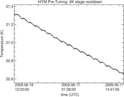
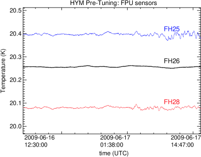
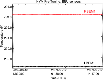
Figure 24: Top panels: thermal behaviour of the 4 K sensor (on the left, HD028260, sampled at 1 Hz, placed in the bottom part of the 4 K thermal shield), Front-End Unit sensors (on the right, FH25, FH26, FH28), bottom panel: Back-End Unit sensors (RBEM-1 and LBEM-1), during the hypermatrix pre-tuning; the Front-End and Back-End sensors position is displayed in Figure 47.

Proper tuning.

The test started on June 19^th at 19:00:00 UTC and was successfully completed on July 9^th at 23:42:32 UTC. It was made of four steps, each corresponding to a different 4 K stage temperature. In Figure 25 we show a plot of the temperature profile of the 4 K stage temperature versus time. Table 6 reports, for each step, the temperature value and drift compared with the test requirements. The r.m.s. temperature variations of the front-end and back-end stages were less than 15 mK and 70 mK, respectively, which did not represent a problem for the tuning analysis.

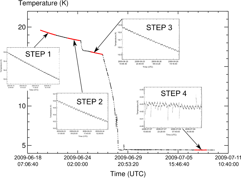
Figure 25: Temperature profile of the 4 K stage during the proper tuning phase. The four insets show the details of the temperature variations during each phase.

Table 6: Average temperatures of the 4 K stage and cooldown speed achieved during the four tuning steps. The average speed is calculated along the whole duration of each step while the maximum speed is calculated during one hour. The last two columns report the required temperature and maximum cooldown rate.

STEP	$T_{\rm start}$	$T_{\rm stop}$	Av. Speed	Max Speed	Req. $T$	Req. max. speed
	(K)	(K)	(mK/h)	(mK/h)	(K)	(mK/h)
1	19.60	19.11	22	27	23.0 $\pm$1.0	40
2	18.61	18.29	20	30	18.0 $\pm$1.0	15
3	16.88	16.55	15	25	15.0 $\pm$1.0	40
4	4.75	4.70	<2	<5	5.0 $\pm$ 0.5	15

For each radiometer, 748 bias quadruplets were explored through the pre-tuning: the resulting noise temperature maps were analysed to identify the new (smaller) bias regions identifying the bias quadruplets to be tested during the proper tuning phase. A baseline set of 22$\times$22=484 quadruplets was selected for each radiometer according to the following rules:

• select bias regions around noise temperature minima measured during pre-tuning;

• select bias regions outside pre-tuning boundaries if there were indications of possible low noise temperatures;

• discard bias quadruplets characterised by drain current imbalance above 25% as this could indicate gain imbalance and poor isolation.

In Figure 26 we show an example of the noise temperature maps with the chosen configurations for the two amplifiers of radiometers LFI21M and LFI24S. In the left panel we see that some of the chosen configurations were selected outside the region tested during the pre-tuning, as the minimum noise temperature was close to the region boundary.

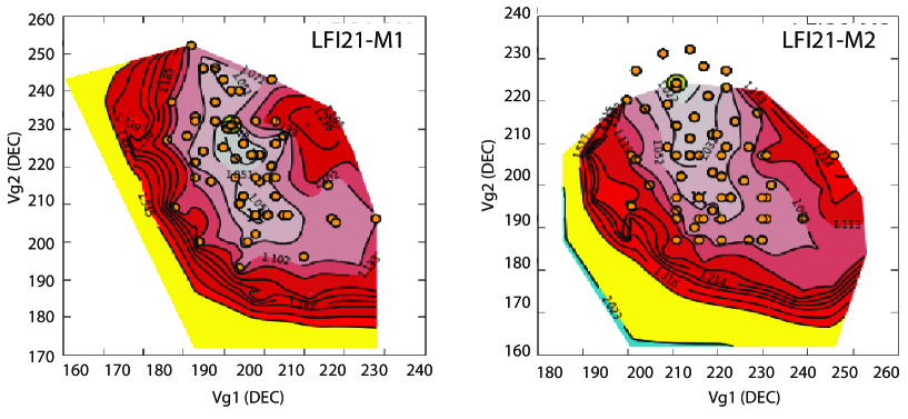
Figure 26: Resampled maps. Noise temperature is displayed for channels LFI21-M1 (left panel) and LFI21-M2 (right panel) as a function of $V_{\rm g1}$, on x-axis, and $V_{\rm g2}$, on y-axis. Colour scale ranges from light blue (highest noise temperatures), through yellow and red to light-grey (lowest noise temperatures), normalized to the lowest noise temperature. Contours represents level of constant noise temperature. Orange bullets in the left and right panels of each channel correspond to the 22 + 22 hand-chosen points, originating the 22$\times$22=484 quadruplets limiting the selected bias sub-region to be resampled. In some cases (as for LFI21-M1), the selected region was contained in the original map; in other cases (as for LFI21-M2), where there was an evidence for a possible improvement, it was chosen out of the boundaries. Note that the bias units are DEC units that are used to set the voltage in the DAE: see Table 4 for a rough conversion into physical units.

This baseline set was enlarged adding the following configurations:

• the 50 quadruplets characterised by the lowest noise temperatures during ground tests [26];

• the 6 optimal bias points found during ground test campaigns and from the drain current verification test described in Section 4.1.3. This allowed a comparison between results taken in the same instrument configuration;

• the 75 quadruplets characterised by the lowest noise temperatures from the pre-tuning analysis;

• 10 points were left available for the procedure optimization. In order to reduce the drift after each bias change, the bias quadruplets were ordered according to the square root sum of the four biases. In correspondence of the ten largest bias steps, the integration time was doubled by setting twice these 10 points.

Noise Temperature, Isolation and Gain balance were measured for each of the 615 independent gate voltage quadruplets of each radiometer.

After having tested all these 615 $V_{\rm gate}$ quadruplets, for each channel we also varied the drain voltage, $V_{\rm drain}$, moving along a subset of bias configurations. For each radiometer we varied three values for $V_{\rm drain,1}$ and three for $V_{\rm drain,2}$ for a subset of 15 $V_{\rm g}$ bias quadruplets testing $3\times 3\times 15$ combinations. The 15 gate voltage quadruplets were chosen among the best results from pre-tuning. This strategy was aimed at an additional fine bias tuning as previously verified during on ground tests performed on Flight Spare Units [26].

To minimize the signal drift due to the bias changes, the duration of each bias step was increased to 20 seconds for the 70 GHz and to 15 seconds for the 30 and 44 GHz channels. The analysis was based only on the last 3 seconds of each step in order to minimize the signal transients.

Each step took about 33 hours; however, the fourth step was completed only after 13 operational days after the end of the 3^rd step (see Figure 25). This delay was partly foreseen in the schedule to comply with HFI activities carried out in the meanwhile, and partly due to 4 K temperature instabilities that required extra investigations and a better stabilization.

Thermal Setup.

Different sensors were used to monitor the 4 K reference Loads, depending on the step and temperature range considered:
- for 1^st, 2^nd and 3^rd steps, the sensor HD028260, placed in the bottom part of the 4 K thermal shield, was used for all the loads as it was the only one provided with calibration curves for temperature above 7 K.
- for the 4^th step, several sensors were available to track the 30/44 GHz and the 70 GHz loads. The Ther-PID4N sensor (placed on the 4 K focal plate) was used to track the 70 GHz loads; the Ther-4KL1 (placed in the middle of the 4 K shield, near LFI25), to track the 30 and 44 GHz loads, assuming a cylindric symmetry of the heat transfer. Data were provided by the HFI Team sampled at 180 Hz and re-sampled at 2 Hz.

As it can be seen in Figure 27, the FPU temperature remained very stable for the whole duration of the tuning tests, preventing changes in Noise and in the Gain at level of the cold LNAs. The Back-End Unit instead suffered some instabilities. They had mostly three causes: (i) the daily perturbations due to the Transponder switch ON/OFF , (ii) the long term drift of the Back End, (iii) perturbation induced in the warm power box of radiometers caused by bias changes. Temperature changes at BEU level induced gain changes in the warm LNAs and offset changes in the warm diodes mimicking true signal changes. These effects (see non linear solution section) were taken into account in the data analysis.

An overview of the thermal conditions (FEU and BEU sensors) during the four hypermatrix tuning steps is given in Appendix F, Table 20.

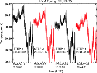
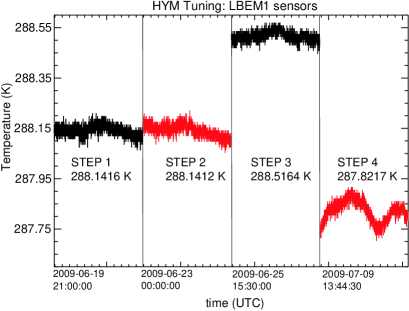
Figure 27: Example showing the FPU (left panel FH25 sensor) and BEU (right panel LBEM1 sensor) thermal stability during the four nominal steps of the hypermatrix tuning. The sensors position is shown in Figure 47. The shape of each curve in the FPU sensors was determined by the changes in power dissipation when changing the bias quadruplets: the four steps exhibited similar thermal conditions. Regarding the BEM curves, the absolute temperature was strongly dependent on the step considered due to the HFI activities performed at 4 K cooler level to keep the required stability during the cooldown and to the transponder ON/OFF effect.

Selection of optimal bias values.

Noise temperature and isolation maps were analysed to find, for each radiometer, the bias configuration yielding optimal performance. Special care was taken to avoid sharp noise temperature minima and bias values with poor isolation and/or unbalanced drain currents. The HYM proper tuning provided in general improved performance with respect to the optimal bias quadruplets resulting from CSL tuning and in most cases the best performing quadruplets were found well inside the four-dimensional sub-regions indicated by the HYM Pre-Tuning. This confirmed the good capability of this technique to provide a resonable guess of the overall performance. Examples of noise temperature maps are provided in Figure 28.

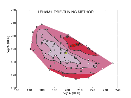
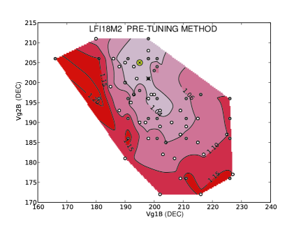
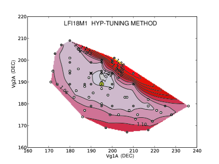
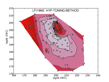
Figure 28: Noise temperature maps for LFI18M as a function of $V_{\rm g1}$, on x-axis, and $V_{\rm g2}$, on y-axis. Comparison between results obtained from pre-tuning approach (based on $Y^{\rm*}$ applied to the 4^th step of HYM), top panels, and from the proper HYM approach (based on Y-factor applied to 1^st and 4^th steps), bottom panels. The condensed noise maps refer to M1 LNA on the left, and to M2 LNA on the right. Colour scale ranges from red (highest noise temperatures) to light-grey (lowest noise temperatures), normalized to the lowest noise temperature. Contours represents level of constant noise temperature. Even if $Y^{\rm*}$ is here calculated from conditions of small thermal unbalance (the input difference between sky and reference was less than 1.7 K in the fourth step), results are comparable. Grey dots correspond to bias pairs common to CSL matrix tuning and to CPV hypermatrix tuning; black crosses correspond to the best performance pairs measured at system level (CSL); yellow circles with black crosses correspond to the best performance pairs measured at CPV level. Note that the bias units are DEC units that are used to set the voltage in the DAE: see Table 4 for a rough conversion into physical units.

In most cases tuning the drain biases did not produce clear improvements, as the shape of the curves was not simple as desired. Drain biases were changed with respect to the ground test default values only when noise temperature improvement was larger than 0.5 K, without degrading Isolation. This happened only in four cases: LFI21M, LFI22M, LFI25M, and LFI28M). The $V_{\rm drain}$ curves for these four radiometers are shown in Figure 29.

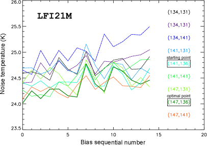
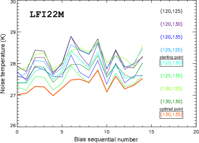
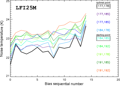
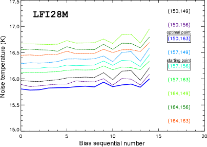
Figure 29: Drain voltage tuning plots: the four plots correspond to the four cases where drain current tuning yielded improved performance. On the abscissa axis we report a sequential number corresponding to each of the 15 $V_{\rm g}$ bias quadruplets under test, on the vertical axis the noise temperature (K). Each curve corresponds to a $V_{\rm drain}$ bias pair, as reported in the legend. Solid thin curves show the noise temperature for the starting point, solid thick curves show the noise temperature for the optimal point.

Comparison to system level tests results.

Direct comparison to results from CSL system level tests (see Figure 30) was possible only over a reduced bias range, covering all the quadruplets common both to CPV and CPV matrices. In many cases maps were well defined and showed a good agreement between the two cases, confirming the validity of the two methods and showing that LFI radiometers did not suffer major changes (complete results are given in Appendix G).

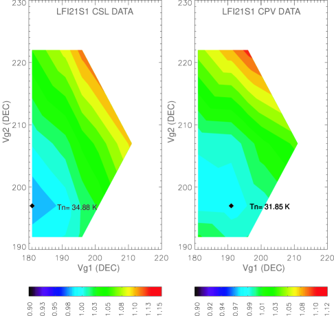
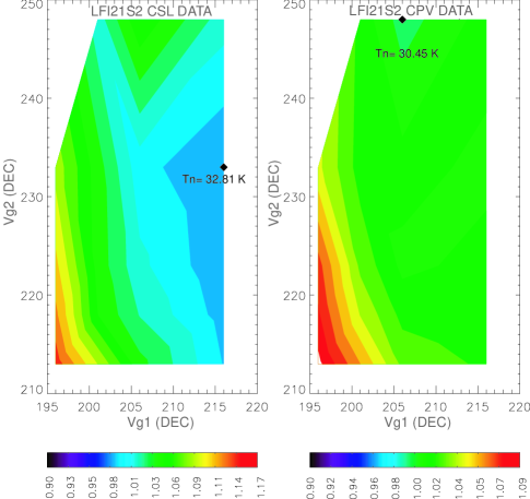
Figure 30: LFI21S1 (top panels) and LFI21S2 (bottom panels) maps are compared in the same bias regions covered by the common quadruplets explored both in CSL system level tests (left panel) and in CPV (right panel): the qualitative agreement is very good, showing the consistency of HYM and the simpler Matrix philosophy used during ground tests. The two dimensional bias spaces shown represent only two slices of the whole four dimensional bias space mapped by hypermatrix tuning. The number of samples depends on the channel and determined the resolution of each map. Note that the bias units are DEC units that are used to set the voltage in the DAE: see Table 4 for a rough conversion into physical units.

In general the resulting biases were very close to ground measured ones, with average variation in $V_{\rm g1}$ and $V_{\rm g2}$ of the order of 1% and few cases where in-flight optimal biases differed from the ground ones by 10-20%. We therefore generally maintained the ground configuration apart from a few cases in which the new configuration provided a noise temperature improvement better than 5% and/or an isolation improvement better than 50% without degrading the 1/$f$ noise performance. Indeed the short integration times for each bias did not allow to evaluate the 1/$f$ noise knee frequency which required at least 1 hour data and was evaluated when tuning was completed.

An unexpectedly high level of $1/f$ noise fluctuations was observed for the 44 GHz RCAs, using either the new flight bias settings or the old ground ones. To test this behaviour we performed several hours of data acquisition with different bias configurations. We observed this instability, both with the in-flight and on-ground optimal biases, only with a particular phase switch configuration of 70 GHz LFI23. We also observed that this instability disappeared, independently from the LFI23 phase switch configuration, when the radiometers were biased with the values resulting from the optimisation of the individual front-end modules before instrument integration (see Figure 31). This interaction between RCAs belonging to different frequency channels was unexpected and the root cause was never fully understood. The most likely explanation was a parasitic oscillation triggered by unexpected cross-talk in the warm electronics.

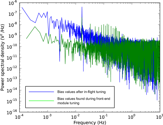
Figure 31: Power spectral density of data from LFI25M-00 detector with two different bias sets. Blue: optimal biases determined after flight tuning tests. Green: optimal biases determined during front-end module tuning before integration.

For this reason this latter final bias setting was chosen for all the 44 GHz radiometers [18]. This setting was characterised by a slightly higher power consumption ($\sim 40$ mW) but similar noise and isolation performance. The power consumption distribution in the two bias frames (optimal bias resulting from hypermatrix tuning and bias default set at the end of the CPV phase) is shown in Figure 33.

In Figure 32 we show the relative variation in noise temperature and isolation for the 30 and 70 GHz receivers between the in-flight and on-ground optimal configurations. From the figure we see that in two cases we had a clear indication of a performance improvement that led us to choose the flight bias settings. These were: LFI18S, for which we obtained a noise temperature reduction larger than 5% and LFI21S for which the noise temperature reduction was limited but the isolation improved by more than a factor of 2 (in dB). Eventually we decided to apply the flight bias setting also to LFI18M which showed a 20% isolation improvement and was close to the 5% threshold we set on noise temperature. For all the remaining receivers we maintained the optimal biases found during satellite on-ground tests. Table 7 summarises the bias settings chosen for the front-end amplifiers at the end of CPV. Concerning the 44 GHz phase switch biases, coherently with the choices done at LNAs level, we decided to apply the unit level test I₁, I₂ values (about 0.8 mA for both, coming from RF-bench optimization). Although the bias region covering these values was not mapped during the CPV (the CPV phase switch tuning focused on a very limited region were the best performance were expected), nevertheless the extrapolated performance from ground data showed that, even if not optimal, this setup was acceptable (Section 4.2.1). At 30 GHz we applied the flight biases that were coincident with ground bias. At 70 GHz, the phase switch setup remained fixed to the default applied since the ground level tests (about 1 mA).
These LNAs and phase switch biases have never been changed since the start of nominal operations.

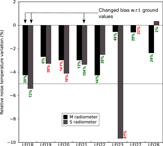
Figure 32: Relative variation in noise temperature and isolation between the flight and ground bias configurations for the 30 and 70 GHz receivers. Negative variation in noise temperature means a smaller noise temperature measured in flight. Green numbers indicate a better isolation measured in flight and red numbers vice-versa. The horizontal line represents the 5% noise temperature improvement threshold.

Table 7: Origin of final bias settings. M and S refer to (V_g1, V_g2) corresponding to Main and Side radiometers. PH/SW identifies the LNAs phase switch bias setup (I₁, I₂) applied to each channel. “Flight” label corresponds to values determined during in-flight tests, “Ground” to satellite-level ground tests, “FEM” to module-level ground tests, “MAX” to maximum current value allowed from specifications and “Gr./Fl.” when Flight and Ground results are coincident.

	Radiometer
RCA	M	S	PH/SW
LFI18	Flight	Flight	MAX
LFI19	Ground	Ground	MAX
LFI20	Ground	Ground	MAX
LFI21	Ground	Flight	MAX
LFI22	Ground	Ground	MAX
LFI23	Ground	Ground	MAX
LFI24	FEM	FEM	FEM
LFI25	FEM	FEM	FEM
LFI26	FEM	FEM	FEM
LFI27	Ground	Ground	Gr./Fl.
LFI28	Gr./Fl.	Ground	Gr./Fl.

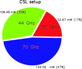
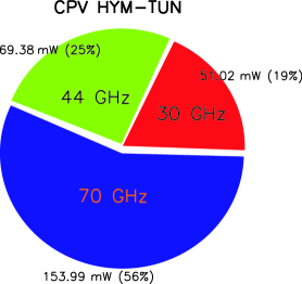
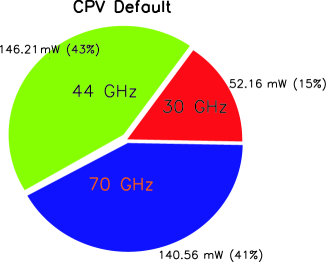
Figure 33: Power consumption distribution among the channels grouped by frequency. The pie charts refer to: the system level tests bias (CSL, top left panel); optimal bias resulting from hypermatrix tuning (top right panel); bias default set at the end of the CPV phase (bottom panel). The corresponding total LFI FPU power consumption was 305.71 mW (CSL), 274.39 mW (hypermatrix) to be compared with the flight conditions of 338.93 mW.

Non linear solution.

The best performance quadruplets were chosen basing the analysis on the Y-factor provided by the linear analysis of the four temperature steps. From the CSL matrix tuning it was already known that the relative improvements in the bias space were only slightly modified by the non linear response of radiometers, only 44 GHz channels showing non linearity effects. Although, as described in the 4.2.2 section, the poor accuracy of the thermometers used during the tuning reduced the sensitivity of the method, nevertheless we applied the non linear model of the Gain [27] to compare with results from the same analysis performed at system level and unit level, and to results from the linear approach. The analysis was applied only to 30 GHz and 44 GHz channels: in fact 70 GHz channels were already known from RCA and system level tests to show a linear response. This analysis was complicated by other effects (for instance the BEU thermal fluctuations, see Figure 27) contributing to masking or generating spurious non linear responses.

Both the linear and the non linear solutions were corrected for the BEU thermal drift along the four steps causing gain changes in the Back-End amplifiers. This correction was applied by imposing the unicity of the sky signal during the four steps of the tuning, neglecting the small variations due to the moving sky and the second order variations due to non perfect Isolation of the LNAs. During the four steps, the Front End temperature remained quite constant, for any given bias quadruplet; the FPU temperature pattern along each step could be ascribed to the different power dissipation of the LNAs, when operated through different bias quadruplets. However, the pattern of instabilities looked repeatable along the four steps (see Figure 27), allowing to consider constant the gain of Front End amplifiers for each quadruplet.
Results confirmed that non linear effects and BEU thermal drift influence only weakly the choice of the optimal biases, apart for those channels (namely the two 30 GHz) showing a very flat response due to the criteria previously adopted to restrict the bias hypermatrix: for these channels only small changes are registered in the noise Temperature when surfing the bias map. For each channel, complete results showing the best bias quadruplets corresponding to the three analysis applied (Linearity, Gain Model, Gain Model considering the Back-End drift correction) are presented in Appendix F, Table 29.

Plots resulting from the non linear Gain-Model analysis corrected for the Thermal Drift of the Back End amplifiers are fully presented in Appendix H. It is worth noting that the correction applied improved w.r.t. the technique described above used in CPV. In fact, data were here corrected on the basis of thermal transfer functions calculated along 40 nominal survey days from August 22^nd to September 30^th, 2009.

Tables reporting the comparison in terms of performance and non linear coefficients among several bias configurations (corresponding to unit level tuning, RCA tuning, CSL system level matrix tuning, CPV default) applied in CPV are reported in Appendix F, Tables 24 to 28.

4.2.3 Tuning verification

Tuning of the LFI has been accomplished at several stages of integration, with different procedures. During these procedures, the system noise temperature (T_sys) and isolation were used as the figures of merit for optimising performance, since they can be estimated with high signal to noise in a short period of time. In fact, for the LFI receivers, the calibrated noise and 1/$f$ characteristics are the true indicators of scientific performance. In principle, calibrated white noise can be derived directly from the system temperature and noise effective bandwidth, but in practice there are noise contributions which make it hard to be sure that white noise predicted by T_sys and bandwidth will be achieved. With a receiver topology as complex as LFI, it is even possible that optimising T_sys and isolation may cause us to miss the actual optimum white noise bias point. With this in mind we developed the following verification test based on the hypermatrix tuning:

• Set LFI for nominal operations (DAE gain and offset tuned to allow measurement of the true radiometer white noise);

• Acquire data (30 seconds) at each of the nominal hypermatrix tuning bias points, in the same manner as was done for the hypermatrix tuning. This samples the LFI bias space around the points most likely to yield good performance;

• Change the 4 K load temperature by a known amount. This change is provided by the HFI team using the PID controller of the 4 K stage;

• Again acquire data at all the hypermatrix bias points;

• White noise is estimated from each 30 second period, and then calibrated using the corresponding data from the known temperature step of the 4 K load.

The results of the white noise hypermatrix are consistent with the normal hypermatrix tuning but provide no extra power to optimise the bias. This result was unexpected. Based on both analytic and monte carlo calculations before flight we estimated only a few percent error in the calibrated white noise, which would have been sufficient.

A possible explanation is in the settling time for the receivers after bias changes. In analyzing this test we allowed a few seconds settling time, but it is possible that the noise characteristics are not stable in this short a time. Given the time limitations on the test, we could not consider larger integration times per bias point, which might have given more stable and discriminatory results.

4.3 Back-end electronics tuning

4.3.1 DAE tuning

The 44 analog voltage outputs from the radiometer back-end modules are digitized in the Digital Acquisition Electronics (DAE) box by 44 14-bit ADCs. The signal $x$ is processed according to the following formula:

$$x\,\textrm{[V]}\quad\rightarrow\quad(x-V_{0})\times G_{\textrm{DAE}}+b_{0}\equiv y\,\text{ [ADU]},$$ (10)

where $V_{0}$ and $G_{\textrm{DAE}}$ are the programmable offset and gain respectively, the latter being responsible for the conversion from Volt to ADU, that is 14-bit integers. The quantity $b_{0}$ is a 14-bit number that depends on the value of $G_{\textrm{DAE}}$. Once the sequence of $y$ is acquired on ground, the Planck-LFI pipeline applies the inverse transformation

$$x=\frac{y-b_{0}}{G_{\textrm{DAE}}}+V_{0}$$ (11)

to reconstruct the signal in Volt.

Each of the 44 ADC converters can be individually programmed. The calibration of the ADCs consists in finding 44 pair of values $(V_{0},G_{\textrm{DAE}})$ satisfying the three following requirements: (i) the voltage $x-V_{0}$ before the amplification stage must be between $-2.5\,\textrm{V}$ and $2.5\,\textrm{V}$, as this is the operating range of the converter; (ii) the value of $G_{\textrm{DAE}}$ should be as large as possible, in order to reduce the quantization noise in the output $y$; (iii) the value of $y$ should not require more than 14 bit (i.e. it must be in the range $[0,2^{14}-1]$), in order to prevent overflows.

We were able to set the value of $V_{0}$ and $G_{\textrm{DAE}}$ by sending telecommands to the DAE which encoded a pair of integer numbers for each ADC. Each integer number matched some specific value for $V_{0}$ and $G_{\textrm{DAE}}$, so that there were 256 different values available for $V_{0}$ and 10 for $G_{\textrm{DAE}}$. The matches between the integer parameters used in the telecommand and the actual values of $V_{0}$ and $G_{\textrm{DAE}}$ were established on ground with a dedicated calibration.

Figure 34: Top panel: plot of the quantity $x_{\textrm{sky}}-x_{\textrm{ref}}$ (reconstructed from $y_{\textrm{sky}}$ and $y_{\textrm{ref}}$ following eq. 11) as a function of the applied offset $V_{0}$, using data acquired at room temperature (sky and reference loads both at 300 K). The balance between the two loads implies that $x_{\textrm{sky}}-x_{\textrm{ref}}$ is roughly zero. The average value does not change while varying $V_{0}$: this proves that we are correctly reconstructing the voltage $x$ from $y$. Bottom panel: when sky and reference load temperatures are unbalanced (sky at 30 K, load at 22 K), the average is no longer zero as expected, but an unexpected spike at $V_{0}\sim 185\,\textrm{DEC}$ reveals the presence of the additional offset $\Delta$ in Eq. (12).

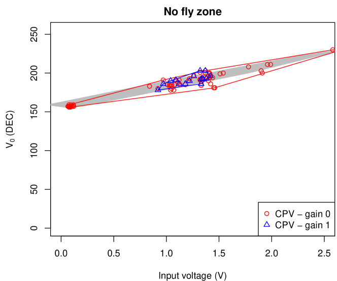
Figure 35: The red and blue points show for which values of the input voltage $V$ entering the ADC the DAE offset $V_{0}$ in eq. (10) introduces an error in the measure. The cloud of points profiles a region in the $V\times V_{0}$ plane called “no-fly zone”. Red points refer to gain state $G_{\textrm{DAE}}=1$, blue to $G_{\textrm{DAE}}=2$ (higher gains are not included as the ADCs saturated before reaching the no-fly zone). The gray region is the no-fly zone measured during the 2006 ground tests (see Figure 18 in [26]). Note the good overlap with the red/blue points.

The “no-fly” zone.

During the LFI ground tests we discovered that for some values of $V_{0}$ (the so-called “no-fly zone”) there was a spurious offset $\Delta$ at the output of the ADC:

$$x\quad\rightarrow\quad(x-V_{0})\times G_{\textrm{DAE}}+b_{0}+\Delta(x,V_{0}),$$ (12)

where the notation $\Delta(x,V_{0})$ stresses that such offset depends both on the input voltage $x$ and the offset $V_{0}$ applied to the DAE (see also [26]). Figure 34 explains this effect by plotting the value of the difference in the voltages $x_{\textrm{sky}}-x_{\textrm{ref}}$ reconstructed on ground using eq. (11), which is not constant as expected when varying the value of $V_{0}$ (taking the difference emphasizes the effect over other systematic effects, most notably slow thermal drifts occurred during the tests).

The presence of $\Delta$ is potentially dangerous for the LFI radiometers, as they are feeding the ADC with pairs of voltages $x_{\textrm{sky}},x_{\textrm{ref}}$ measuring the temperature of two mismatched loads (the sky at 2.7 K and the reference load at 4.5 K): therefore, picking a value of $V_{0}$ for which $\Delta\not=0$ would lead to a difference $\Delta_{\textrm{sky}}-\Delta_{\textrm{ref}}$ that is not cancelled by the differential strategy.

We empirically found a region in the $x\times V_{0}$ plane producing nonzero $\Delta$: such values $V_{0}^{\textrm{no-fly}}$ depend on the input voltage $x$. For all those detectors showing enough low noise we were able to clearly identify two pairs $(x,V_{0}^{\textrm{no-fly}})$ corresponding respectively to sky signal $x_{\textrm{sky}}$, and to reference signal $x_{\textrm{ref}}$. Figure 35 compares CPV results (in the $x\times V_{0}$ plane) to those obtained during on ground tests (2006). The consistency of results from the two tests , proved the stability with time of this effect and its independence from the environmental conditions (laboratory/space) and from the applied gain $G_{\textrm{DAE}}$.

Even if we did not understand the real cause of this spurious offset $\Delta$, we were able to produce a “safe” calibration for LFI by picking $V_{0}$ values not falling into the no-fly zone.

Calibration methodology.

The calibration of the DAE was divided into two parts:

1. Calibration. Data were acquired while exercising the 44 ADC converters in each possible configuration; such data were used to determine the best values for $V_{0}$ and $G_{\textrm{DAE}}$ for each converter.

   This phase required the REBA to acquire 30 seconds data in AVR1 uncompressed mode (see Section 4.3.2) for each of the possible gain and offset states of the DAE ($10\times 255=2\,550$ states). The negligible cross-talk between the 44 ADCs allowed to change their state in parallel. The full test required about 21 hours ($2\,550\times 30\,\,\textrm{s}$).

2. Verification. Performed after having uploaded the best configuration in the DAE. It simply required to acquire data for a few minutes to verify the consistency of output from each ADC with analytical predictions. Figure 36 shows the ranges of variation of the voltages during the First Light Survey.

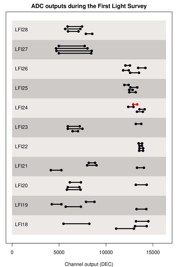
Figure 36: Range of variations of the scientific output (i.e. $y_{\textrm{sky/ref}}$ in eq. 10) for the 44 LFI channels. For each RCA the four diodes are (from the lowest to the topmost): M-00, M-01, S-10, S-11. The time considered for the production of the plot is the so-called “First Light Survey”, which lasted 15 days. Since an unexpected gain change provoked a saturation in channel LFI24S-11 (marked with red) during the first days of the first light survey, in this case we discarded the first three days of the first light survey in computing the range.

Figure 37: The values of the DAE offset $V_{0}$ (eq. 10) resulting from the DAE calibration adopted for the nominal survey were chosen well out of the no-fly zone (gray polygon). $V_{0}$ is plotted against the average value of the sky (black points) and reference (gray points) signals $x_{\textrm{sky}}$ and $x_{\textrm{ref}}$ ($44\times 2=88$ points). The horizontal bars show the typical range of variation of the output during the first 2 years of data acquisition. For clarity, the gray points have been shifted horizontally by +1.

Figure 38: Top panel: the measured standard deviation (s.d.) of the digital data produced by the ADC of the channel LFI24M-00 (44 GHz) during the DAE calibration test as a function of the applied gain. We chose to show LFI24M-00 as it has a low intrinsic output ($\sim$ 0.4 V) and therefore did not saturate even when applying the maximum gain $G_{\textrm{DAE}}=15$. Note the expected linear correlation between the r.m.s. of the data and the gain. Botton panel: Unlike 30 and 70 GHz channels, 44 GHz channels like LFI24M-00 show an increase in the r.m.s. level of their differenced output which is correlated with the value of $V_{0}$ ($G_{\textrm{DAE}}$ was kept constant at 0 DEC, the lowest gain state). For further details, see text.

The results of the DAE calibration can be schematized as follows:

• For each detection line, the set of pairs $(G_{\textrm{DAE}},V_{0})$ for which the ADC saturates were measured and are consistent with our analytical models.

• The increase in the r.m.s. of the signal is well correlated with the ADC gain (see e.g. LFI24M-00 in the top plot in Figure 38), as it was expected (note we were able to check this property only for those channels with a voltage output small enough to exercise all the gain states without saturating the ADC).

• The r.m.s. did not change while varying the ADC offset $V_{0}$, except for the 44 GHz channels (see the bottom plot in Figure 38). These channels are characterized by an unusually low output ($\sim$0.1 V), which therefore allows to detect the noise of the ADC itself. This was hardly a problem, as the main purpose of $V_{0}$ in this context was to make the signal entering the ADC close to zero: for the 44 GHz channels the small signal allowed us to pick up $V_{0}=0\,\mathrm{V}$, thus avoiding the problem.

• The best configuration $(G_{\textrm{DAE}},V_{0})$ was chosen for each ADC in order to maximize the gain while keeping the ADC far from saturating. The ADCs were proven to be within the allowed limits during the period called “First Light Survey” (corresponding to the Operational Days 91–105 corresponding to August 12^th to 26^th, 2009). Also, the value for $V_{0}$ was always chosen to be far enough from the no-fly zone (see Figure 37).

• We had the proof that the no-fly zone effect is remarkably stable, as from the analysis of the CPV tests we found the very same results of the RAA test campaign (which was performed three years before). Also, since for the first time we were able to study this effect for every value of the gain $g$, we finally had the proof that the shape of the no-fly zone does not depend on $G_{\textrm{DAE}}$. See Figure 35.

4.3.2 REBA tuning

The LFI Signal Processing Unit is a module of the REBA whose purpose, among others, is to downsample and compress the scientific data acquired by the radiometers and digitized by the DAE at a sampling rate of $\approx 8$ kHz, in order to fit the spacecraft telemetry bandwidth. Preprocessing includes a downsampling stage and a tunable lossy compression scheme which allows to achieve high compression ratios ($C_{\mathrm{r}}\sim 2.4$) at the expense of increasing the noise level. Details on the full preprocessing and compression stage, as well as its optimization and characterization are given in [14].Since the preprocessing plus compression is tunable by defining a set of 4 parameters for each detection line ($\mathcal{O}$, $S_{\mathrm{q}}$, $r_{1}$ and $r_{2}$), the objective of the REBA tuning was to find the set of 44 quadruplets that allowed to fit the total bandwidth within the requirements while keeping the digitization noise and other possible distortions as low as possible [14].

The calibration and verification of the REBA compressor exploits the ability of the REBA to acquire each LFI detector in two modes at the same time, that is in AVR1 mode (the ground station receives the data after they are downsampled but before they enter the compression stage) or COM5 mode (ground receives the data after the compression stage). Due to inflight bandwidth constrains, it is not possible to make all the 44 detectors work in AVR1 mode, in the nominal configuration of LFI all the detectors work in COM5 mode while in turn one detector is sampled also in AVR1 for half an hour realizing a round–robin scheme whith a 22 hours cycle.

Here are the stages of the REBA optimization done during the CPV:

1. The nominal round–robin scheme was switched off.

2. Each of the 44 detectors was kept in stable conditions and data were acquired in AVR1 mode for 45 minutes. To save time, 11 detectors were acquired at the same time, so that the overall duration of the data acquisition phase was only three hours.

3. Using the software suite and the optimization methods reported in [14], for each detector statistics of downsampled signals was derived and used to asses a first analytical pre–optimization.

4. We further optimized the compression configurations on the uncompressed data acquired exploring a regularly gridded subset of each of 4-dimensional parameter space around the pre optimized parameter sets.

5. To determine the best configuration, we used the following criteria: (1) the compression ratio $C_{\mathrm{r}}$ must be not smaller than the requirement, which is 2.4; (2) the quantization error on a weighted averages of the sky and reference signals measured by the detector must be the lowest one. Both the $C_{\mathrm{r}}$ and the quantization errors are measured on the real data by using a software which reproduces both the onboard production of COM5 data out of the AVR1 data and the subsequent decompression and decoding at the Ground Segment.

6. Once the best configuration was found, the procedure repeated from step 4 by centering the grid in the parameter space around this configuration and by shrinking it 10 times along each of the four dimensions. This produced a new “best” configuration. We compared the compression ratios, quantization levels and required bandwidths of the two “best” configurations in order to make the final choice.

7. After the REBA was programmed with the quadruplets found in the previous step, the instrument was put in nominal mode and started with the nominal round–robin for a 22 hours cycle.

8. The 22 hours of data were analysed in order to check if the differences between the AVR1 and COM5 datastreams for each radiometers were in agreement with the analysis done in step 4.

The results of the test were satisfactory. All the 44 channels were able to compress the data so that the overall compression ratio was $C_{\mathrm{r}}\approx 2.4$, corresponding to the requirement. The quantization induced by the compressor accounted for a $\sim 5\%$ increase in the r.m.s. level, which is considered to be acceptable.

4.4 Performance and calibration

After the instrument was fully tuned its noise performance was assessed during a dedicated test that was split into two parts:

1. a data acquisition performed with the radiometers unswitched, where the noise spectra were compared for all four phase switch configurations. The objective of this test was to assess whether any phase switch configuration was preferable from the point of 1/$f$ noise;

2. a data acquisition with the radiometers nominally switching in order to characterise the full noise properties in both switching configurations (A/C or B/D), with the twin phase switch in its nominal position. Photometric calibration was performed using the CMB dipole allowing a preliminary assessment of the in-flight white noise instrument sensitivity.

The instrument thermal configuration was nominal. The front-end unit temperature ranged from 19.6 K to 20.6 K with a stability of $\pm 5$ mK, the 4 K stage was at $4.37\pm 0.002$ K and the back-end unit temperature ranged from 287.7 K to 309.8 K with a stability of $\pm 0.1$ K.

4.4.1 Noise properties with radiometers unswitched

This test consisted in four acquisitions of 20 minutes each, in order to test all the phase switch configurations. The only exception was the LFI23 receiver for which the B/D phase switches were always kept in the 0 position to avoid the anomalous 1/$f$ noise described in Section 4.1.1 (Figure 9). In all cases the 4 kHz switching was set to zero for both A/C and B/D. The complete set of phase switch configurations tested is summarised in Table 8.

Table 8: Phase switch configurations during the four acquisitions with the radiometers unswitched. The configurations relative to LFI23 are marked in boldface because for that receiver the B/D switches were always kept in the 0 position to avoid the anomalous noise level triggered by the B/D=1 configuration (see Section 4.1.1, Figure 9).

	Configuration 1				Configuration 2
RCA	A/C pos	B/D pos		RCA	A/C pos	B/D pos
LFI18	1	0		LFI18	0	0
LFI19	1	0		LFI19	0	0
LFI20	1	0		LFI20	0	0
LFI21	1	0		LFI21	0	0
LFI22	1	0		LFI22	0	0
LFI23	1	0		LFI23	0	0
LFI24	1	0		LFI24	0	0
LFI25	1	0		LFI25	0	0
LFI26	1	0		LFI26	0	0
LFI27	1	0		LFI27	0	0
LFI28	1	0		LFI28	0	0
	Configuration 3				Configuration 4
RCA	A/C pos	B/D pos		RCA	A/C pos	B/D pos
LFI18	0	1		LFI18	1	1
LFI19	0	1		LFI19	1	1
LFI20	0	1		LFI20	1	1
LFI21	0	1		LFI21	1	1
LFI22	0	1		LFI22	1	1
LFI23	0	0		LFI23	1	0
LFI24	0	1		LFI24	1	1
LFI25	0	1		LFI25	1	1
LFI26	0	1		LFI26	1	1
LFI27	0	1		LFI27	1	1
LFI28	0	1		LFI28	1	1

In Figure 39 we show two examples of noise amplitude spectral density plots relative to detectors LFI19M-00 and LFI27M-00. In each plot we have overplotted spectra from all four configurations with different colours (black for configuration 1, red for configuration 2, blue for configuration 3 and green for configuration 4). The four spectra essentially overlap showing that any extra noise introduced by the phase switch is equivalent in the four possible switch states.

The remaining forty-two plots not shown in this paper reproduce the same behaviour of the two examples presented here. Therefore we have not included them for simplicity.

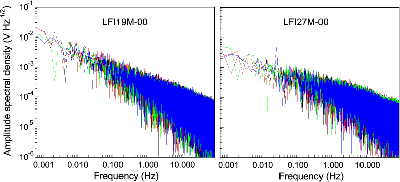
Figure 39: Amplitude spectral density plots from LFI19M-00 and LFI27M-00 detectors data acquired with radiometers unswitched. Each plot contains spectra from all four possible phase switch configurations (red, green, blue and black lines). Spectra overlap, showing that the four configurations are equivalent in terms of noise contribution. Spectra from all the other detectors are equivalent to those presented here and are not shown for simplicity.

4.4.2 Noise properties with radiometers switched

This test consisted in two 12-hour acquisitions in nominal bias and thermal conditions in order to check for 1/$f$ noise differences determined by the switching configuration. In Table 9 we list the two switching configurations tested. Notice that the switching configuration of LFI23 was not changed because of the anomalous noise caused by the configuration with B/D switching. Therefore LFI23 did not change configuration in the two acquisitions and could be used as a repeatability verification channel.

Table 9: Phase switch configurations in the two data acquisitions for noise characterisation. The receiver LFI23, which did not change configuration, is highlighted in boldface.

Configuration 1					Configuration 2
RCA	4 kHz sw.	Fixed sw.	pos.		RCA	4 kHz sw.	Fixed sw.	pos.
LFI18	B/D	A/C	1		LFI18	A/C	B/D	0
LFI19	B/D	A/C	1		LFI19	A/C	B/D	0
LFI20	B/D	A/C	1		LFI20	A/C	B/D	0
LFI21	B/D	A/C	1		LFI21	A/C	B/D	0
LFI22	B/D	A/C	1		LFI22	A/C	B/D	0
LFI23	A/C	B/D	0		LFI23	A/C	B/D	0
LFI24	B/D	A/C	0		LFI24	A/C	B/D	0
LFI25	B/D	A/C	0		LFI25	A/C	B/D	0
LFI26	B/D	A/C	0		LFI26	A/C	B/D	0
LFI27	B/D	A/C	0		LFI27	A/C	B/D	0
LFI28	B/D	A/C	1		LFI28	A/C	B/D	0

Differences in 1/$f$ noise in the two switching configurations.

In Figure 40 we show the percent difference in 1/$f$ knee frequency for the two tested configurations. Positive numbers indicate that knee frequencies in configuration 2 are larger and vice versa. If we consider a 10% level of repeatability as indicated by LFI23 we see that, in general, in configuration 1 the noise was more stable (smaller knee frequencies). The only noticeable exceptions were represented by LFI26 and LFI24M for which the displayed knee frequency was smaller in configuration 2.

Because configuration 1 was more extensively tested during the whole test campaign and the 1/$f$ level of LFI26 in this configuration was still compatible with the MADAM map-making code [17, 28], we eventually preferred configuration 1 as the default switching configuration for all receivers.

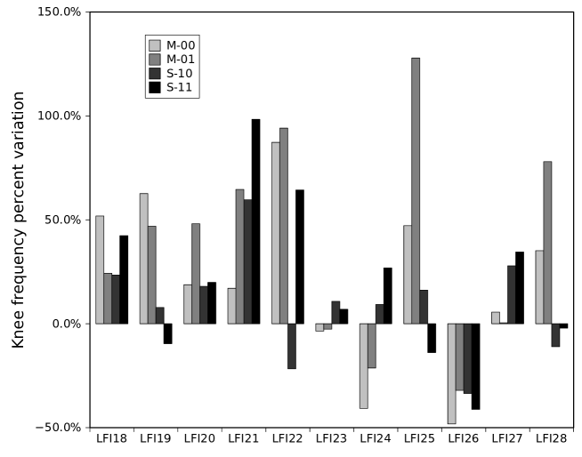
Figure 40: Percent variation in knee frequency between the two phase switch configurations ($\delta=(f_{\rm k}^{\mathrm{Conf\,2}}-f_{\rm k}^{\mathrm{Conf\,1}})/f_{\rm k}^{\mathrm{Conf1}}$). The variation in LFI23 can be considered as a reference for the repeatability of this comparison, as the phase switch configuration was not changed for this receiver.

In Table 10 we list the measured knee frequencies in mHz for all 44 LFI detectors in the default switching configuration. For a more detailed discussion about the 1/$f$ noise performance measured during nominal operations see [8].

Table 10: Knee frequencies in mHz measured in flight during CPV.

	M-00	M-01	S-10	S-11
LFI18	52	58	43	50
LFI19	47	49	79	86
LFI20	32	28	45	43
LFI21	56	45	45	30
LFI22	51	44	81	43
LFI23	104	76	58	60
LFI24	65	48	60	48
LFI25	29	25	39	45
LFI26	105	71	117	111
LFI27	105	119	83	67
LFI28	79	64	62	61

Photometric calibration.

The CMB Doppler dipole anisotropy induced by Earth and spacecraft motions with respect to the CMB rest frame was used as a calibrator to convert the voltage output into antenna temperature units. The nominal calibration procedure and accuracy has been discussed in detail in [8, 17] and will not be repeated here. It is worth mentioning that during CPV tests a simplified calibration pipeline was used, in which a 20^∘ galactic cut was applied to the data to remove the galactic signal, but no iterative algorithm was implemented to estimate and remove the CMB anisotropy.

In Figure 41 we show the calibration constants as measured in flight during CPV ($x$-axis) compared to those measured on ground during satellite tests ($y$-axis) where we used temperature variations of a 4 K black-body load that illuminated the focal plane and simulated the sky cold load. In the figure we report the comparison only for the receivers that were biased with the same voltages (see Table 7). The figure shows a broad agreement between the two calibration constant sets with systematically larger values measured in flight, with differences ranging from $\sim 2\%$ to $\sim 17\%$ depending on the receiver. Because differences in calibrated white noise were found to be less than 5% (see Figure 42) we believe that differences in calibration constant values indicated different values of the receiver gains probably due to slightly different bias voltages at the cold amplifiers compared to the ground test environment.

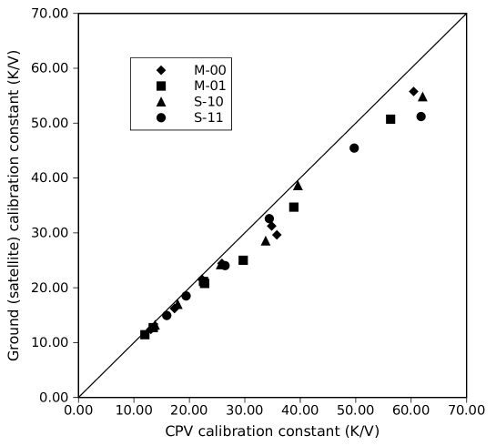
Figure 41: Photometric calibration constants measured in flight during CPV ($x$-axis) and on ground during satellite tests ($y$-axis).

White noise performance.

Figure 42 shows the white noise sensitivity in antenna temperature units measured in flight during CPV compared with measurements performed on ground during satellite tests. The comparison show a remarkable agreement apart from three outstanding cases: LFI21S-10, LFI21S-11 and LFI24M-00. For these three channels the white noise sensitivity improved by 24%, 30% and 15%, respectively, due to improved bias tuning. For all remaining channels the agreement was better than 10% with a median discrepancy of about 2%.

This showed that we were able to generally match the ground-measured instrument sensitivity performance [22] while improving on a small subset of channels. More detailed discussion on the stability of the sensitivity performance during the first year of operations is provided in [8].

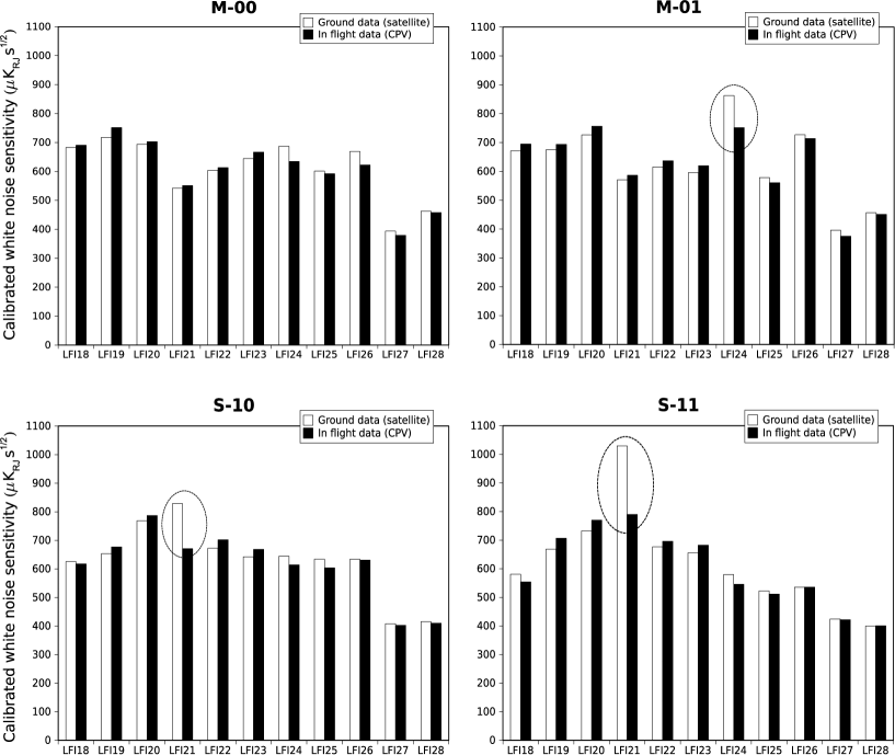
Figure 42: White noise sensitivities in antenna temperature measured on ground (satellite) and in flight (CPV). Sensitivity increased for LFI21S-10, LFI21S-11 and LFI24M-01 (circled bars) thanks to in-flight improved bias tuning.

4.5 Thermal susceptibility

The effect of temperature fluctuations on the LFI radiometers is originated in the Planck cold end interface of the hydrogen sorption cooler to the instrument focal plane, the LVHX2. The temperature is actively controlled through a dedicated stage, the TSA, providing a first reduction of the effect. The thermal mass of the focal plane strongly contribute to reduce residual fluctuations.

The physical temperature fluctuations propagated at the front end modules cause a correlated fluctuation in the radiometer signal degrading the quality of scientific data. The accurate characterization of this effect is crucial for possibly removing it from raw data by exploiting the housekeeping information of thermal sensors. The propagation of the temperature oscillations through the focal plane and the instrument response to thermal changes were characterized through two main tests performed during CSL system level tests and verified in the latest part of the CPV (instruments already tuned, in nominal configuration): the thermal dynamic response [29] and the radiometers thermal susceptibility [30].

4.5.1 Dynamic thermal verification

This test was aimed at measuring the dynamic thermal behaviour of the LFI Focal Plane; it started on July 29^th at 6:00 UTC with a duration of four hours. In order to amplify the effect and to get a more accurate measurement, the active control from the TSA was switched off. The resulting increased fluctuations, propagating at the cooler frequencies, were used to evaluate transfer functions between the TSA stage and the FPU sensors (Figures 43 and 44). The analysis, conducted following the two methods reported in [29], produced damping factors of 2–5 at about 1 mHz .

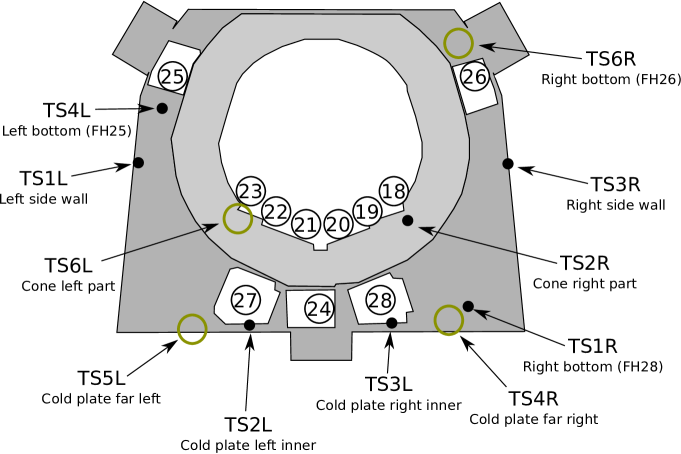
Figure 43: Schema of the focal plane sensor locations. Sensor TS5R FH28 Flange, not included here, is located on the flange of LFI28 horn.

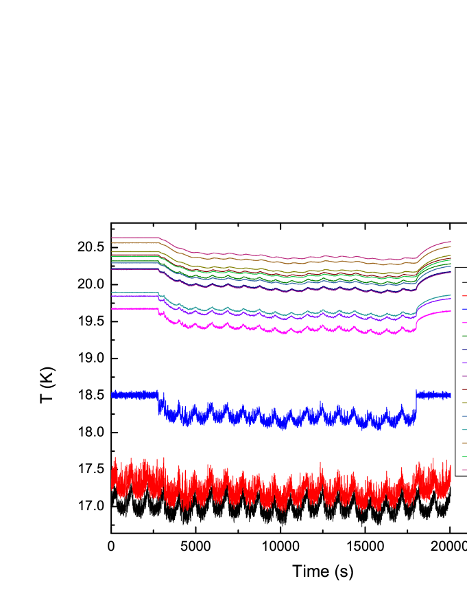
Figure 44: Dynamic behaviour of the sensors when TSA control is switched off; fluctuations at 1 mHz are reduced more than 40%.

The source of fluctuations was characterized by two typical periods of the sorption cooler during the final CPV phase: (i) the single bed cycle time, 940 s, (ii) the complete cooler period, six times larger, 5640 s.

The first analysis method consisted in performing a Discrete Fourier Transfom (DFT) of the sensor timestreams. The second method consisted in fitting the sensor timestreams with a double sinusoidal function: ${\rm T(t)=T_{0}+A1\cdot sin(2\pi\nu_{1}t+\phi_{1})+A2\cdot sin(2\pi\nu_{2}t+\phi_{2})}$ where ${\rm\nu_{1}}$ = 1/940 Hz and ${\rm\nu_{2}}$ = 1/5640 Hz. In both methods transfer functions were evaluated by the ratio of the resulting amplitudes and by the phase differences at the considered frequencies.

Figure 45 shows the time stream available for the analysis in the frequency domain: this method did not allow to efficiently sample the lowest frequency peak and a comparison between the two methods is possible only for the 940 s component. Results from both methods are in agreement, as shown in the Table 11 reporting data from the sinusoidal fit together with relative differences between the two methods. Sorting the sensors by the transfer function amplitudes in descending order (second column of the table), the route of the propagation of temperature fluctuations through the focal plane sensors (shown in Figure 43) was reproduced as expected: the largest amplitudes are in the sensor closest to the right bottom corner interface with the working cooler and they decrease in the direction left upwards. The measured values in flight are compared to what measured during the ground test at satellite level in Figure 46, showing good agreement. The 20% difference in the phase measured at the time scale of 5640 s is coherent with a larger uncertainty in the fit for a dataset including just about 1.5 times the fluctuation period (about two hours of data were used).

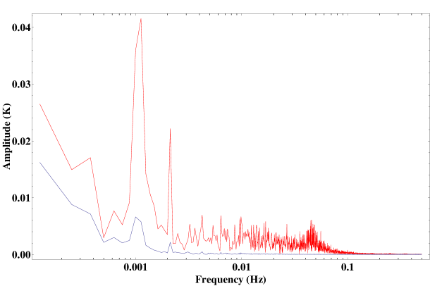
Figure 45: Fourier transform comparison of TSA sensor (red line) with one of the sensors in the left side of the focal plane, TS2L (blue line).

Table 11: Transmission amplitudes and phases of fluctuations at the two main cooler frequencies during the transient test. Results are taken from the double sinusoidal fit method (see text and references). Typical fit parameters uncertainties are at 1% level. In the last two columns relative differences between the results of the two methods at 1 mHz are reported.

	Results 1.064 mHz		Results 0.177 mHz		Compare $\sim$1 mHz
Sensor ID	Ampl.	Phase (rad)	Ampl.	Phase (rad)	rel. ${\rm\Delta}$ Amp (%)	rel. ${\rm\Delta\phi}$ (%)
TSL1	0.113	1.79	0.520	0.95	0	11
TSL2	0.153	1.13	0.560	0.81	9	7
TSL3	0.266	0.60	0.600	0.60	5	0
TSL4	0.112	1.83	0.522	0.96	1	11
TSL5	0.136	1.37	0.554	0.87	8	9
TSL6	0.110	1.70	0.483	0.98	2	12
TSR1	0.402	0.33	0.660	0.41	2	3
TSR2	0.218	0.86	0.583	0.68	6	2
TSR3	0.222	0.84	0.589	0.68	6	1
TSR4	0.313	0.49	0.616	0.52	4	2
TSR5	0.224	0.84	0.586	0.68	6	1
TSR6	0.158	1.23	0.545	0.81	8	7

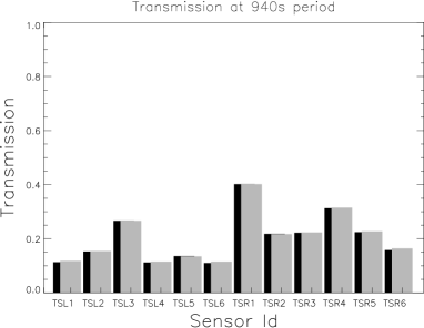
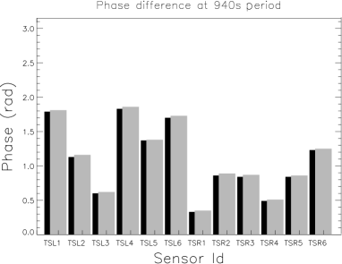
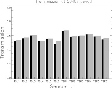
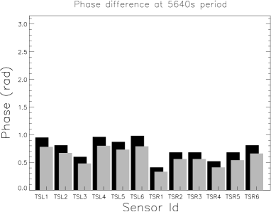
Figure 46: Comparison between CPV (black bars) and CSL (grey bars) measurements of amplitude (left panels) and phase (right panels) of the transfer functions for the single bed fluctuation period of 940 s (top panels) and for the whole cooler fluctuation period of 5640 s (bottom panels).

4.5.2 Thermal susceptibility

Fluctuations of the focal plane temperature would cause variations of important parameters (mainly the low noise amplifier gains and noise temperatures), impacting the radiometer output signal, as detailed in [30]. The response of the LFI radiometers to thermal fluctuations was estimated by inducing discrete temperature steps on the focal plane through TSA setpoint changes. The test started on August 11^th at 9:15 UTC. The setpoint was changed over four values (Figure 47, left) and after a stabilization of at least two hours, the measured receivers output was characterized as a function of each temperature variation of about 0.3 K. Due to reduced duration of the DTCP, the temperature steps were performed during two consecutive visibility periods. At the beginning of the first DTCP, a major temperature step up ($\Delta T\approx+0.8$ K) was performed while the TSA setpoint was decreased of a step downwards just before the loss of visibility with the spacecraft. in order to guarantee that the heat load on the sorption cooler interface was at the lowest possible level during the long period of 20 hours with no direct monitoring.

The slope of the resulting ${\rm T_{ant}}$ vs ${\rm T_{phys}}$ plot is the measured response of the receivers to a change in the temperature (Figure 47, bottom).

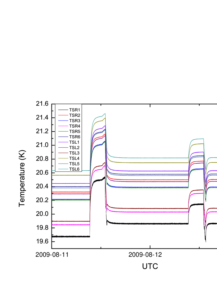
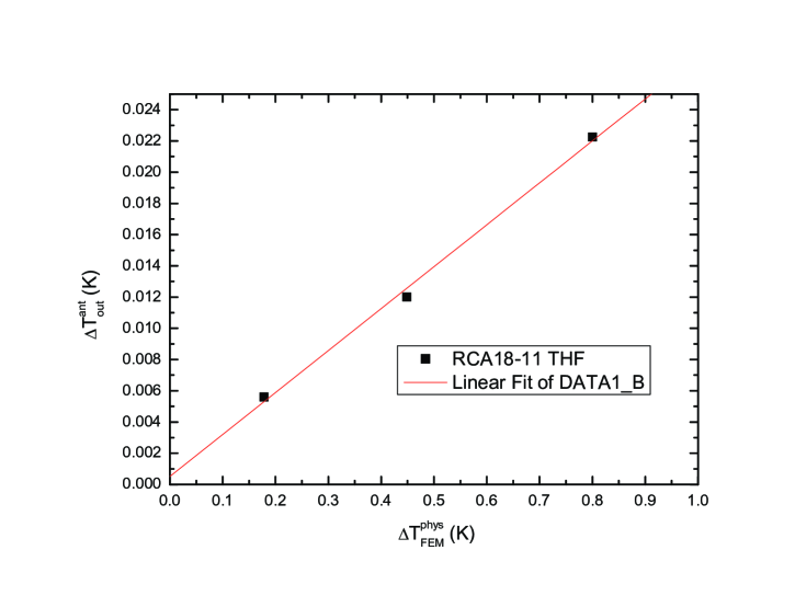
Figure 47: Top panel: overall view of the LFI sensors in the final part of the susceptibility test. Bottom panel: the slope of the fitted line is a measure of the signal variation as a function of changing focal plane temperature.

Results, reported in the Table 12, confirmed that physical temperature fluctuations in the main frame are furtherly reduced when convolved with the radiometer thermal susceptibility coefficients: the derived output fluctuations, measured in antenna temperature, were actually reduced by an extra factor of 10 to 200 (according to the channel considered), of the same order of ground test results [30]. This corresponds to reduce the mean peak-to-peak amplitudes of fluctuations measured by high resolution sensors, of the order of 4 mK in steady condition, of at least one order of magnitude in the output timestream.

Figure 48 shows the same results in two separate plots, one for each radiometer Main and Side. Values from coupled detectors are in general in line with the above considerations: the main parameters affected by the temperature changes are noise and gain of the amplifier chain, which is shared by the two coupled diodes of each radiometer. LFI28 showed a different behaviour: the calibrated susceptibilities measured for the two coupled diodes are non consistent within the error bars. It is worth noting that LFI28 shows very peculiar features in terms of high $r$ (see eq. 3) factors and asymmetry between the paired detectors: even if the above inconsistency can not be univocally related to these features, it is likely that they are contributing to generate it.

Table 12: Results of thermal susceptibility test. Units are K_ant/K_phys. Together with the radiometers, the closest sensor used as reference for the physical temperature is indicated. Results for the detector LFI24S-11 are missing because it suffered a period of signal saturation during the test.

Radiometer (sensor)	M-00	M-01	S-10	S-11
LFI18 (TS2R)	0.040 $\pm$ 0.010	0.030 $\pm$0.010	0.031 $\pm$ 0.009	0.027 $\pm$ 0.009
LFI19 (TS2R)	0.040 $\pm$ 0.010	0.050 $\pm$0.010	0.030 $\pm$ 0.010	0.040 $\pm$ 0.010
LFI20 (TS2R)	0.050 $\pm$ 0.010	0.060 $\pm$0.010	0.040 $\pm$ 0.010	0.050 $\pm$ 0.010
LFI21 (TS6L)	0.029 $\pm$ 0.009	0.039 $\pm$0.009	0.060 $\pm$ 0.010	0.070 $\pm$ 0.010
LFI22 (TS6L)	0.080 $\pm$ 0.010	0.069 $\pm$0.009	0.100 $\pm$ 0.010	0.100 $\pm$ 0.010
LFI23 (TS6L)	0.050 $\pm$ 0.010	0.040 $\pm$0.010	0.050 $\pm$ 0.010	0.050 $\pm$ 0.010
LFI24 (TS2L)	0.013 $\pm$ 0.008	0.013 $\pm$0.009	0.014 $\pm$ 0.007	–
LFI25 (TS4L)	0.012 $\pm$ 0.007	0.008 $\pm$0.007	0.001 $\pm$ 0.007	0.001 $\pm$ 0.007
LFI26 (TS6R)	-0.020$\pm$ 0.008	-0.009$\pm$ 0.009	0.006 $\pm$ 0.008	0.010 $\pm$ 0.007
LFI27 (TS2L)	-0.007$\pm$ 0.005	0.000 $\pm$0.005	-0.007 $\pm$ 0.005	0.001 $\pm$ 0.005
LFI28 (TS5R)	0.041 $\pm$ 0.006	0.027 $\pm$0.006	0.034 $\pm$ 0.005	0.011 $\pm$ 0.005

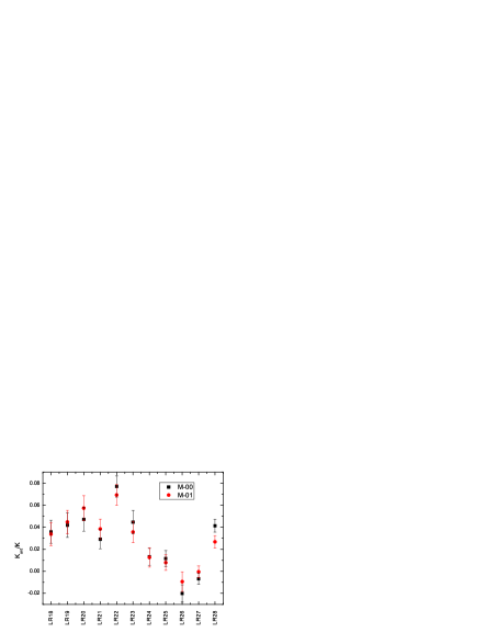
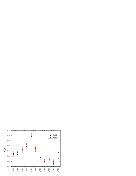
Figure 48: Results of the susceptibility test for the RCAs main arm (left panel) and side arm (right panel) radiometers.

5 Conclusions

We have summarized the overall CPV plan of Planck-LFI, designed to ensure proper in-flight verification and tuning of all the key element of the instrument. The plan was designed taking into account the constraints and the opportunities provided by the gradual cool-down of the various interfaces of the instrument assembly after launch. The functionality of the key LFI subsystems, as well as of the instrument as a whole, was repeatedly verified in-flight in a wide range of conditions, including and expanding over those covered by ground tests. Spurious 1-Hz spikes and I-V response of the LNAs were measured for all radiometers and compared with results from ground tests. The results show good repeatability of the instrument behaviour.

A rather sophisticated tuning procedure was operated on the main LFI subsystems to maximise the instrument scientific performance. We exploited the cool-down of the 4K stage to calculate noise temperature and isolation in a large parameter space of LNA biases (the so-called hypermatrix tuning) and identified optimal parameter sets. We also tuned phase switch currents to reach optimal balance. We tuned the DAE gain and offset to optimise the voltage input at the ADC for each LFI channel. Finally, we set the REBA parameters to optimise the tradeoff between digital quantisation and compression efficiency.

As soon as the instrument was operational, and well before the beginning of the first light survey, we used the CMB dipole signal to routinely perform a first-order photometric calibration, which allowed us to monitor the main instrument performance (white noise, 1/f noise) during CPV. As expected, the photometric calibration and noise parameters were somewhat different from those measured on the ground. However, accounting for the somewhat different thermal and electrical interfaces, the agreement is very good.

A crucial aspect in the understanding of the LFI behaviour is the sensitivity of the radiometers response to changes in the thermal interfaces. In particular, we have extensively measured the transfer functions coupling the radiometric response to temperature variations in the focal plane by switching off the stabilisation PID of the 20 K stage. This measurement provides a key informaiton for analysis of systematic effects. While thermal tests were carried out also on-ground, the stability of the space environment in L2 allowed us to obtain much more accurate results in the CPV campaign.

Overall the CPV campaign has shown excellent consistency with the results of ground tests, and in general it has yielded improved accuracy. All the calibration activities were performed successfully and yielded very satisfactory results leading to a slightly improved LFI performance compared to ground tests.

Appendix A Channel grouping tables

Table 13: Grouping of LFI channels in power groups: channels belonging to each power group share the same power box. This grouping has been used during CRYO-01 test.

Power Group	Channels
1	LFI 18, LFI 26
2	LFI 19, LFI 20, LFI 28
3	LFI 21, LFI 22, LFI 24, LFI 27
4	LFI 23, LFI 25

Table 14: Grouping of LFI Channels used during the drain current test.

Power Group	Channels
1	LFI 18, LFI 21
2	LFI 19, LFI 22
3	LFI 20, LFI 23
4	LFI 25, LFI 24
5	LFI 26, LFI 27
6	LFI 28

Table 15: Grouping of LFI channels used during LNAs hypermatrix pre-tuning and proper tuning.

Power Group	Channels
1	LFI 18, LFI 19, LFI 22
2	LFI 20, LFI 21, LFI 23
3	LFI 24, LFI 26, LFI 28
4	LFI 25, LFI 27

Appendix B Sequence of steps in CRYO-01 functionality tests

Table 16: Sequence of steps performed during the CRYO-01 test.

Step	Description	Expected response
1	The first ACA is biased with LNAs and phase switch biases ($V_{\rm g1}$, $V_{\rm g2}$, $V_{\rm d}$, $I_{1}$, $I_{2}$)	The signal rises on the pair of output diodes connected to the ACA†
2	The phase switch polarisation is changed	The signal switches from sky to reference load or vice versa
3	The 4 kHz switching is activated	From each diode two output streams appear with different voltage outputs.
4	The phase switch bias current $I_{1}$ is lowered	The separation between the two datastreams changes (either they converge or they diverge)
5	The phase switch bias current $I_{1}$ is returned to its nominal value and $I_{2}$ is lowered	The separation changes in the opposite direction
6	$I_{2}$ is returned to its nominal value, the 4 kHz switching is turned off and the phase switch state is returned to 0	The signal returns as after step 1‡
7	The second ACA is biased with LNAs and phase switch biases ($V_{\rm g1}$, $V_{\rm g2}$, $V_{\rm d}$, $I_{1}$, $I_{2}$)	The output voltage increases in both diodes†
8	The phase switch polarisation is changed	The signal switches from sky to reference load or vice versa
9	The 4 kHz switching is activated	From each diode two output streams appear with different voltage outputs.
10	The phase switch bias current $I_{1}$ is lowered	The separation between the two datastreams changes (either they converge or they diverge)
11	The phase switch bias current $I_{1}$ is returned to its nominal value and $I_{2}$ is lowered	The separation changes in the opposite direction
12	$I_{2}$ is returned to its nominal value, the 4 kHz switching is turned off and the phase switch state is returned to 0	The signal returns as after step 1‡

^† Drain current is recorded and compared to ground test CSL values.
^‡ Here the output voltage can be different because of drifts caused by the thermal environment and amplifier stabilisation.

Appendix C Plots of 1 Hz frequency spikes

In Figure 49 we show the amplitude spectral density of 1 Hz frequency spikes in all the LFI outputs measured during on-ground and in-flight tests with radiometers completely unbiased.

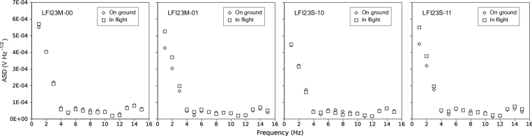
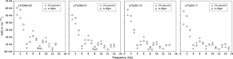
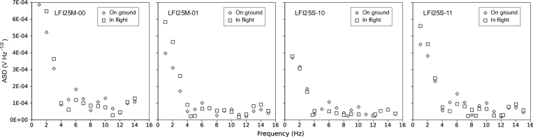
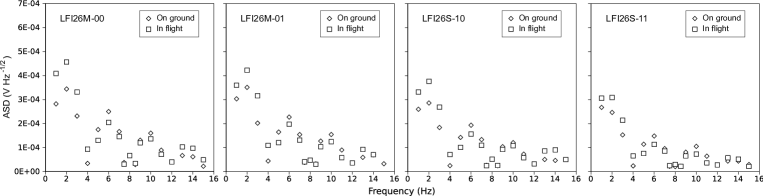
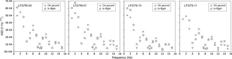
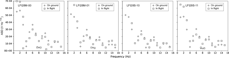
Figure 49: ASD of 1 Hz frequency spikes detected in the warm electronics noise and measured on-ground and in-flight with the radiometers left unbiased. All 44 output channels are shown. Two anomalous spikes were detected in the two outputs LFI22M-00 and LFI22M-01.

Appendix D Plots of drain current

In Figure 50 we show for all the LFI channels the I-V curves (for each diode); black lines (“plus sign” symbols) refer to system level tests data measured in CSL, blue lines (“cross” symbols) refer to the $1^{\rm st}$ and red lines (“triangle” symbols) to the $3^{\rm rd}$ run performed during CPV.

LFI-18

LFI-19

LFI-20

LFI-21

LFI-22

LFI-23

LFI-24

LFI-25

LFI-26

LFI-27

LFI-28

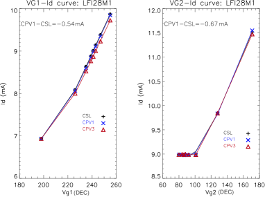
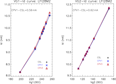
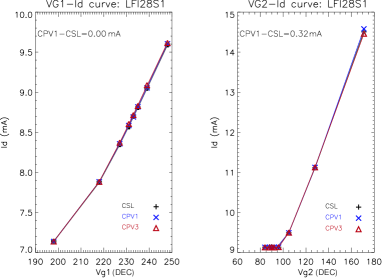
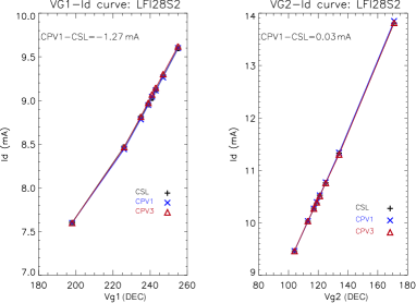
Figure 50: I-V curves: for each channel $V_{\rm g1}$ and $V_{\rm g2}$ plots are both shown. Black “plus sign” symbols refer to system level tests results in CSL; blue “crosses” to CPV 1^st run, red “triangles” to the 3^rd run. Solid lines represent the corresponding polynomial fits. Curves from the CSL system level tests and CPV 1^st run are offset to facilitate the comparison; the offset terms are print on top left of each picture. Note that the bias units are DEC units that are used to set the voltage in the DAE: see Table 4 for a rough conversion into physical units.

Appendix E Phase switch labelling and tuning maps

In Table 17 we show the correspondance between LNA names (M1, M2, S1, S2) and the corresponding phase switch pairs (A/C, B/D) and BEM output diodes (M-00, M-01, S-10, S-11) for all RCAs.

Table 17: Phase switch correspondance to LNAs and BEM diodes.

RCA	Amplifier	Phase switch state	Detector
	& Phase switch	& 4 kHz
LFI18	S2	A/C	S-10; S-11
	S1	B/D
	M1	A/C	M-00; M-01
	M2	B/D
LFI19	S2	A/C	S-10; S-11
	S1	B/D
	M1	A/C	M-00; M-01
	M2	B/D
LFI20	S2	A/C	S-10; S-11
	S1	B/D
	M1	A/C	M-00; M-01
	M2	B/D
LFI21	S2	A/C	S-10; S-11
	S1	B/D
	M1	A/C	M-00; M-01
	M2	B/D
LFI22	S2	A/C	S-10; S-11
	S1	B/D
	M1	A/C	M-00; M-01
	M2	B/D
LFI23	S2	A/C	S-10; S-11
	S1	B/D
	M1	A/C	M-00; M-01
	M2	B/D
LFI24	M2	A/C	M-00; M-01
	M1	B/D
	S2	A/C	S-10; S-11
	S1	B/D
LFI25	M1	A/C	M-00; M-01
	M2	B/D
	S1	A/C	S-10; S-11
	S2	B/D
LFI26	M2	A/C	M-00; M-01
	M1	B/D
	S2	A/C	S-10; S-11
	S1	B/D
LFI27	M1	A/C	M-00; M-01
	M2	B/D
	S1	A/C	S-10; S-11
	S2	B/D
LFI28	M1	A/C	M-00; M-01
	M2	B/D
	S1	A/C	S-10; S-11
	S2	B/D

In Figure 51 we show for the 30 GHz and 44 GHz LFI channels the condensed noise temperature maps corresponding to the linear hypermatrix tuning analysis: these maps were used as input to select the optimal bias.

LFI-24

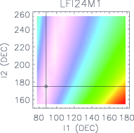
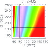
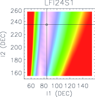
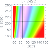
LFI-25

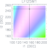
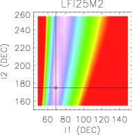
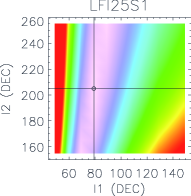
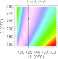
LFI-26

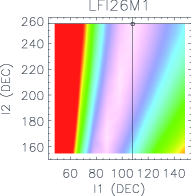
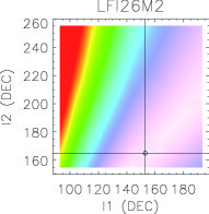
LFI-27

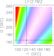
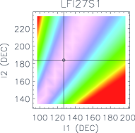
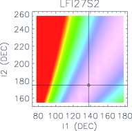
LFI-28

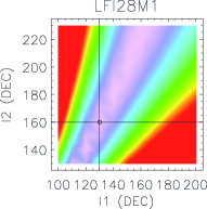
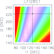
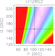
Figure 51: Phase switch tuning maps. For each channel they are represented from left to right panels the detectors: M1, M2, S1, S2. I₁ bias lies on x-axis, I₂ bias on y-axis. The color scale shows smaller umbalance in bright and larger unbalance in dark. Values are normalized to the average signal output. The intercept of the two lines indicates the optimal bias selected. Note that the bias units are DEC units that are used to set the bias in the DAE: see Table 5 for a conversion into physical units.

Appendix F Collection of tables with detailed test results

Table 18: Phase switch tuning bias: optimal bias (Opt) compared to best values (Best) from automatic procedure and to system level test results (Csl). Values are given in the decimal units that are used to set the bias in the DAE: see Table 5 for a conversion into physical units.

	Opt		Best		CSL
	I1	I2	I1	I2	I1	I2
LFI24M1	98	215	88	175	128	250
LFI24M2	77	185	77	185	77	205
LFI24S1	84	235	84	235	84	235
LFI24S2	86	205	86	205	86	215
LFI25M1	154	245	154	245	174	235
LFI25M2	79	255	69	175	89	250
LFI25S1	79	205	79	205	89	250
LFI25S2	119	225	119	225	119	225
LFI26M1	108	255	108	255	98	245
LFI26M2	153	165	153	165	153	210
LFI26S1	135	235	135	235	135	230
LFI26S2	93	225	93	225	93	230
LFI27M1	148	220	148	220	178	180
LFI27M2	145	205	124	165	144	214
LFI27S1	127	184	127	184	117	154
LFI27S2	148	195	138	175	128	200
LFI28M1	130	160	130	160	150	204
LFI28M2	127	228	97	148	105	164
LFI28S1	127	222	127	222	111	168
LFI28S2	103	165	103	165	93	155

Table 19: Hypermatrix tuning timeline in operational days (OD) starting from the Launch date.

STEP	OD Start	OD Stop	Time Start (UTC)	Time Stop (UTC)
1	37	38	2009-06-19 19:00:00	2009-06-21 04:12:32
2	40	41	2009-06-22 22:00:00	2009-06-24 07:12:32
3	43	44	2009-06-25 13:30:00	2009-06-26 22:42:32
4	55	56	2009-07-07 13:30:00	2009-07-08 22:42:32

Table 20: Average values and sigma measured from FPU and BEU sensors during the four steps of the hypermatrix tuning.

		STEP 1		STEP 2		STEP 3		STEP 4
NAME	PARAM	T	sigma	T	sigma	T	sigma	T	sigma
FPU sensors (units are K)
CONE R	LM302332	20.211	0.008	20.209	0.008	20.207	0.008	20.209	0.008
CONE L	LM206332	20.488	0.011	20.486	0.011	20.483	0.011	20.485	0.011
FH28 Fl	LM305332	20.084	0.008	20.083	0.008	20.081	0.008	20.083	0.008
FH26 R	LM306332	20.260	0.011	20.258	0.011	20.255	0.011	20.256	0.011
FH25 L	LM204332	20.400	0.012	20.397	0.012	20.394	0.012	20.394	0.012
BEU sensors (units are K)
LBEM1	LM207332	288.141	0.022	288.141	0.024	288.516	0.019	287.822	0.041
LBEM2	LM208332	290.640	0.019	290.641	0.024	291.027	0.018	290.308	0.044
RFEM1	LM309332	292.605	0.051	292.567	0.051	292.955	0.053	292.256	0.08
RFEM2	LM310332	288.819	0.011	288.825	0.014	289.154	0.013	288.434	0.045
LFEM1	LM209332	292.481	0.057	292.499	0.062	292.875	0.057	292.208	0.067
LFEM2	LM210332	288.129	0.017	288.133	0.022	288.509	0.017	287.810	0.041
RBEM2	LM308332	288.366	0.011	288.366	0.015	288.695	0.012	287.963	0.042
RBEM1	LM307332	290.891	0.010	290.902	0.013	291.246	0.012	290.519	0.043

Table 21: Average Noise Temperature (K) and Isolation from 30 GHz and 44 GHz channels hypermatrix tuning: comparison between CSL and CPV results.

	24M	24S	25M	25S	26M	26S	27M	27S	28M	28S
Noise Temperature (K)
CSL	21.8	23.3	24.3	22.8	26.9	23.05	16.8	18.2	16.2	15.5
CPV	20.3	21.2	21.7	20.0	25.0	21.0	16.7	18.2	15.8	15.5
Isolation
CSL	0.011	0.0285	0.016	0.002	0.044	0.012	0.0085	0.004	0.029	0.044
CPV	0.011	0.0275	0.015	0.001	0.028	0.011	0.0065	0.005	0.023	0.043

Table 22: Average Noise Temperature (K) and Isolation from 70 GHz channels hypermatrix tuning: comparison between CSL and CPV results.

	18M	18S	19M	19S	20M	20S	21M	21S	22M	22S	23M	23S
Noise Temperature (K)
CSL	28.1	27.6	29.6	26.3	32.3	29.0	32.5	24.0	28.6	27.8	31.7	30.5
CPV	26.6	26.5	28.6	25.6	31.0	28.2	30.1	23.3	27.9	26.6	28.8	28.4
Isolation
CSL	N.A.	N.A.	0.026	N.A.	0.027	0.0187	0.167	0.0235	0.038	-0.001	0.010	0.025
CPV	0.035	0.029	0.027	0.041	0.032	0.0145	0.021	0.0215	0.028	-0.001	0.025	0.015

Table 23: Optimal average noise temperature T_n (K) and Isolation (Isol) resulting from different tuning phases: optimal bias from ground tests (CSL), from CPV HYM using only gate voltages V_g (TUN) and from the full HYM tests, including the drain voltage V_d part (SET). Results are given in terms of V_d pairs and V_g 1,2 quadruplets (in decimal values): Noise Temperature (K) and Isolation (dB) averaged over the two coupled diodes, drain currents (mA) of the two coupled ACAs (Id_1,2). Voltage units are decimal: conversion in volts can be roughly obtained referring to Table 4.

	Phase	(Vd,1,Vd,2)	(Vg 1,1,Vg 2,1),(Vg 1,2,Vg 2,2)	Tn	Isol	Id1	Id2
21M	CSL	(141, 136)	(198, 207) , (196, 197)	24.05	-16.40	18.42	19.56
	TUN	=	(192, 240) , (194, 232)	24.69	-19.20	21.92	25.54
	SET	(147, 136)	(192, 231) , (191, 224)	23.30	-16.70	21.54	23.87
22M	CSL	(125, 130)	(203, 194) , (178, 176)	28.14	-19.80	14.16	14.94
	TUN	=	(218, 210) , (188, 188)	28.06	-20.20	18.49	18.10
	SET	(130, 135)	(208, 218) , (188, 188 )	26.64	-23.50	18.87	18.53
23S	CSL	(118, 122)	(181, 211) , (190, 208)	31.89	-19.20	20.83	15.16
	TUN	=	(184, 213) , (198, 213)	30.31	-15.51	21.34	17.09
	SET	(123, 127)	(180, 222) , (198, 213)	28.78	-16.00	21.77	17.74
25M	CSL	(184, 185)	(227, 212) , (219, 212)	24.32	-17.72	9.4	10.04
	TUN	=	(223, 203) , (211, 200)	23.28	-19.00	6.65	6.78
	SET	(177, 178)	(231, 203) , (218, 200)	21.75	-18.20	6.28	6.28
28M	CSL	(157, 156)	(243, 101) , (240, 112)	16.30	-15.50	9.62	9.15
	TUN	=	(243, 101) , (240, 112)	16.30	-15.50	9.62	9.15
	SET	(150, 163)	(243, 101) , ( 240, 112)	15.87	-16.40	8.99	9.77

Table 24: LFI-24 Tuning: Gain-Model results^†. Results from several sets of biases tested during the CPV are compared among each other and to ground test results (RCA paper [21]). For each radiometer (separately Main and Side) and for each detector (labelled with 1, 2) the gain model parameters are shown on the right side of the table: noise temperatures $T\rm_{n}$ (given in K), the non-linear coefficients $b$ (adimensional) and the Gains $G$ (expressed as V/K). Corresponding values corrected for the BEU thermal drift are reported on the right side (G.M. correction). The bias settings considered are optimal biases from: RCA test campaign (RCA), unit level test campaign (FEM), system level test campaign (CSL), hypermatrix tuning (CPV).

	Main Radiometer
	Gain model						G.M.correction
SOURCE	$T\rm_{n,1}$	$b_{1}$	$G_{1}$	$T\rm_{n,2}$	$b_{2}$	$G_{2}$	$T\rm_{n,1}$	$b_{1}$	$G_{1}$	$T\rm_{n,2}$	$b_{2}$	$G_{2}$
RCA Paper	N.A.	N.A.	N.A.	N.A.	N.A.	N.A.	15.5	1.794	0.0048	15.3	1.486	0.0044
RCA	24.3	-0.34	0.0031	23.1	-0.57	0.0031	17.0	1.46	0.0050	16.7	0.99	0.0051
FEM	24.1	-0.29	0.0032	23.0	-0.57	0.0032	16.7	1.51	0.0051	16.6	1.03	0.0051
CSL	23.7	-0.53	0.0028	25.1	-0.41	0.0037	16.3	1.58	0.0045	16.3	0.99	0.0044
CPV	27.3	-2.99	0.0016	27.3	-1.53	0.0026	15.4	2.21	0.0032	15.0	1.86	0.0032
	Side Radiometer
	Gain model						G.M.correction
SOURCE	$T\rm_{n,1}$	$b_{1}$	$G_{1}$	$T\rm_{n,2}$	$b_{2}$	$G_{2}$	$T\rm_{n,1}$	$b_{1}$	$G_{1}$	$T\rm_{n,2}$	$b_{2}$	$G_{2}$
RCA PAPER	N.A.	N.A.	N.A.	N.A.	N.A.	N.A.	15.8	1.44	0.0062	15.8	1.45	0.0062
RCA	24.3	-0.34	0.0031	25.5	-0.26	0.0046	17.2	0.88	0.0072	17.4	0.95	0.0079
FEM	24.1	-0.29	0.0032	23.0	0.16	0.0088	17.4	0.87	0.0073	18.1	0.82	0.0076
CSL	25.1	-0.69	0.0037	22.9	-0.93	0.0028	16.0	1.11	0.0066	16.1	1.19	0.0072
CPV	25.2	-1.37	0.0026	25.0	-2.55	0.0015	15.4	1.33	0.0049	15.6	1.41	0.0053

^† A gain model was developed based on the results of Daywitt (1989), modified for the LFI [27]. The total power output voltage $V_{\rm out}$ can be written as:

$$V_{\rm out}=\frac{G}{1+b\cdot G\cdot(T_{\rm in}+T_{\rm n})}\cdot(T_{\rm in}+T_{\rm n})$$ (14)

where $T_{\rm in}$ is $T_{\rm sky}$ or $T_{\rm ref}$, $T_{\rm n}$ the noise temperature (K), $G$ the total gain (V/K) in the case of a linear radiometer, $b$ the linear coefficient.

Table 25: LFI-25 Tuning: Gain-Model results. Results from several sets of biases tested during the CPV are compared among each other and to ground test results (RCA paper [21]). For each radiometer (separately Main and Side) and for each detector (labelled with 1, 2) the gain model parameters are shown on the right side of the table: noise temperatures $T\rm_{n}$ (given in K), the non-linear coefficients $b$ (adimensional) and the Gains $G$ (expressed as V/K). Corresponding values corrected for the BEU thermal drift are reported on the right side (G.M. correction). The bias settings considered are optimal biases from: RCA test campaign (RCA), unit level test campaign (FEM), system level test campaign (CSL), hypermatrix tuning (CPV).

	Main Radiometer
	Gain model						G.M.correction
SOURCE	$T\rm_{n,1}$	$b_{1}$	$G_{1}$	$T\rm_{n,2}$	$b_{2}$	$G_{2}$	$T\rm_{n,1}$	$b_{1}$	$G_{1}$	$T\rm_{n,2}$	$b_{2}$	$G_{2}$
RCA PAPER	N.A.	N.A.	N.A.	N.A.	N.A.	N.A.	17.5	1.22	0.0086	17.9	1.17	0.0085
RCA	22.6	0.33	0.0073	23.7	0.09	0.0073	14.8	1.25	0.0124	16.2	1.03	0.0104
FEM	21.9	0.49	0.0087	23.3	0.22	0.0087	14.9	1.21	0.0140	16.2	1.01	0.0118
CSL	22.3	0.34	0.0073	23.4	0.09	0.0073	15.1	1.21	0.0118	16.5	0.99	0.0099
CPV	20.7	0.39	0.0054	21.6	0.16	0.0054	12.3	1.89	0.0101	13.2	1.73	0.0088
	Side Radiometer
	Gain model						G.M.correction
SOURCE	$T\rm_{n,1}$	$b_{1}$	$G_{1}$	$T\rm_{n,2}$	$b_{2}$	$G_{2}$	$T\rm_{n,1}$	$b_{1}$	$G_{1}$	$T\rm_{n,2}$	$b_{2}$	$G_{2}$
RCA PAPER	N.A.	N.A.	N.A.	N.A.	N.A.	N.A.	18.6	0.80	0.0079	18.4	1.01	0.0071
RCA	23.5	0.05	0.0081	23.0	0.15	0.0081	16.9	0.71	0.0125	15.3	1.05	0.0120
FEM	22.3	0.19	0.0088	23.0	0.16	0.0088	15.9	0.83	0.0135	15.4	1.05	0.0119
CSL	22.4	0.07	0.0072	N.A.	N.A.	N.A.	16.0	0.83	0.0110	14.9	1.13	0.0102
CPV	20.8	-0.19	0.0034	N.A.	N.A.	N.A.	10.7	2.67	0.0074	10.1	3.16	0.0068

Table 26: LFI-26 Tuning: Gain-Model results. Results from several sets of biases tested during the CPV are compared among each other and to ground test results (RCA paper [21]). For each radiometer (separately Main and Side) and for each detector (labelled with 1, 2) the gain model parameters are shown on the right side of the table: noise temperatures $T\rm_{n}$ (given in K), the non-linear coefficients $b$ (adimensional) and the Gains $G$ (expressed as V/K). Corresponding values corrected for the BEU thermal drift are reported on the right side (G.M. correction). The bias settings considered are optimal biases from: RCA test campaign (RCA), unit level test campaign (FEM), system level test campaign (CSL), hypermatrix tuning (CPV).

	Main Radiometer
	Gain model						G.M.correction
SOURCE	$T\rm_{n,1}$	$b_{1}$	$G_{1}$	$T\rm_{n,2}$	$b_{2}$	$G_{2}$	$T\rm_{n,1}$	$b_{1}$	$G_{1}$	$T\rm_{n,2}$	$b_{2}$	$G_{2}$
RCA PAPER	N.A.	N.A.	N.A.	N.A.	N.A.	N.A.	18.4	1.09	0.0052	17.4	1.42	0.0067
RCA	27.8	-0.29	0.0046	25.5	0.65	0.0046	19.7	0.84	0.0073	14.8	1.73	0.0143
FEM	26.9	-0.15	0.0046	25.3	0.66	0.0046	19.5	0.91	0.0071	15.3	1.73	0.0133
CSL	27.7	-0.56	0.0034	26.3	0.41	0.0034	18.6	1.12	0.0059	14.6	2.02	0.0108
CPV	26.3	-0.68	0.0026	23.4	0.68	0.0026	15.5	2.16	0.0052	10.7	3.28	0.0102
	Side Radiometer
	Gain model						G.M.correction
SOURCE	$T\rm_{n,1}$	$b_{1}$	$G_{1}$	$T\rm_{n,2}$	$b_{2}$	$G_{2}$	$T\rm_{n,1}$	$b_{1}$	$G_{1}$	$T\rm_{n,2}$	$b_{2}$	$G_{2}$
RCA PAPER	N.A.	N.A.	N.A.	N.A.	N.A.	N.A.	16.8	0.94	0.0075	16.5	1.22	0.0082
RCA	22.3	-0.13	0.0056	23.7	0.083	0.0056	14.5	1.07	0.0095	16.2	1.08	0.0097
FEM	22.7	-0.14	0.0060	24.3	0.05	0.0060	14.9	0.94	0.0101	16.6	0.98	0.0103
CSL	22.6	-0.16	0.0059	24.8	-0.0470	0.0059	15.2	0.89	0.0097	17.1	0.90	0.0098
CPV	21.9	-0.53	0.0028	23.2	-0.38	0.0028	9.9	3.24	0.0070	11.8	2.72	0.0067

Table 27: LFI-27 Tuning: Gain-Model results. Results from several sets of biases tested during the CPV are compared among each other and to ground test results (RCA paper [21]). For each radiometer (separately Main and Side) and for each detector (labelled with 1, 2) the gain model parameters are shown on the right side of the table: noise temperatures $T\rm_{n}$ (given in K), the non-linear coefficients $b$ (adimensional) and the Gains $G$ (expressed as V/K). Corresponding values corrected for the BEU thermal drift are reported on the right side (G.M. correction). The bias settings considered are optimal biases from: RCA test campaign (RCA), unit level test campaign (FEM), system level test campaign (CSL), hypermatrix tuning (CPV).

	Main Radiometer
	Gain model						G.M.correction
SOURCE	$T\rm_{n,1}$	$b_{1}$	$G_{1}$	$T\rm_{n,2}$	$b_{2}$	$G_{2}$	$T\rm_{n,1}$	$b_{1}$	$G_{1}$	$T\rm_{n,2}$	$b_{2}$	$G_{2}$
RCA PAPER	N.A.	N.A.	N.A.	N.A.	N.A.	N.A.	12.1	0.12	0.0723	11.9	0.12	0.0774
RCA	15.4	0.03	0.0776	16.1	0.02	0.0786	13.7	0.06	0.0934	13.7	0.06	0.1015
FEM	16.0	0.02	0.0774	16.2	0.02	0.0774	13.8	0.06	0.0911	13.8	0.0564	0.0992
CSL	15.4	0.03	0.0765	15.5	0.03	0.0765	13.2	0.07	0.0904	13.2	0.0672	0.0992
CPV	15.4	0.03	0.0776	16.6	0.02	0.0675	13.2	0.07	0.0927	13.3	0.06	0.0998
	Side Radiometer
	Gain model						G.M.correction
SOURCE	$T\rm_{n,1}$	$b_{1}$	$G_{1}$	$T\rm_{n,2}$	$b_{2}$	$G_{2}$	$T\rm_{n,1}$	$b_{1}$	$G_{1}$	$T\rm_{n,2}$	$b_{2}$	$G_{2}$
RCA PAPER	N.A.	N.A.	N.A.	N.A.	N.A.	N.A.	13.0	0.13	0.0664	12.5	0.14	0.0562
RCA	18.7	0.01	0.0687	16.8	0.0132	0.0687	15.6	0.06	0.0855	14.3	0.06	0.0733
FEM	18.8	0.01	0.0660	16.9	0.01	0.0660	15.9	0.06	0.0808	14.5	0.06	0.0699
CSL	18.4	0.02	0.0674	16.7	0.01	0.0674	15.5	0.06	0.0828	14.3	0.06	0.0704
CPV	18.2	0.02	0.0675	16.6	0.02	0.0675	15.4	0.07	0.0829	14.2	0.07	0.0701

Table 28: LFI-28 Tuning: Gain-Model results. Results from several sets of biases tested during the CPV are compared among each other and to ground test results (RCA paper [21]). For each radiometer (separately Main and Side) and for each detector (labelled with 1, 2) the gain model parameters are shown on the right side of the table: noise temperatures $T\rm_{n}$ (given in K), the non-linear coefficients $b$ (adimensional) and the Gains $G$ (expressed as V/K). Corresponding values corrected for the BEU thermal drift are reported on the right side (G.M. correction). The bias settings considered are optimal biases from: RCA test campaign (RCA), unit level test campaign (FEM), system level test campaign (CSL), hypermatrix tuning (CPV).

	Main Radiometer
	Gain model						G.M.correction
SOURCE	$T\rm_{n,1}$	$b_{1}$	$G_{1}$	$T\rm_{n,2}$	$b_{2}$	$G_{2}$	$T\rm_{n,1}$	$b_{1}$	$G_{1}$	$T\rm_{n,2}$	$b_{2}$	$G_{2}$
RCA PAPER	N.A.	N.A.	N.A.	N.A.	N.A.	N.A.	10.6	0.19	0.0621	10.3	0.16	0.0839
RCA	14.9	0.03	0.0647	14.2	0.04	0.0647	12.7	0.08	0.0771	12.4	0.0735	0.1028
FEM	15.7	0.02	0.0598	15.2	0.03	0.0598	13.2	0.07	0.0728	13.0	0.07	0.0958
CSL	15.7	0.01	0.0597	14.7	0.03	0.0597	13.0	0.07	0.0735	12.6	0.07	0.0984
CPV	15.7	0.01	0.0597	14.7	0.03	0.0597	13.0	0.07	0.0735	12.6	0.07	0.0984
	Side Radiometer
	Gain model						G.M.correction
SOURCE	$T\rm_{n,1}$	$b_{1}$	$G_{1}$	$T\rm_{n,2}$	$b_{2}$	$G_{2}$	$T\rm_{n,1}$	$b_{1}$	$G_{1}$	$T\rm_{n,2}$	$b_{2}$	$G_{2}$
RCA PAPER	N.A.	N.A.	N.A.	N.A.	N.A.	N.A.	9.9	0.19	0.0607	9.8	0.20	0.0518
RCA	15.8	0.01	0.0573	14.8	0.01	0.0573	13.3	0.07	0.0692	9.9	0.14	0.0792
FEM	16.0	0.01	0.0566	14.9	0.01	0.0566	13.5	0.07	0.0689	9.7	0.15	0.0815
CSL	15.9	0.01	0.0564	14.7	0.03	0.0597	13.3	0.07	0.0686	9.7	0.14	0.0804
CPV	15.7	0.01	0.0540	15.7	0.01	0.0540	13.1	0.07	0.0663	9.4	0.16	0.0782

Table 29: Optimal biases resulting from HYM Maps when the Linear Model (LIN), the Gain Model (G.M.) and the Gain Model corrected (labelled as G.M.+C) for the BEU thermal drift are applied. Voltage units are decimal values: conversion in Volts can be roughly obtained referring to Table 4.

	LIN	G.M.	G.M.+C
RCA	$V\rm_{g1}$ , $V\rm_{g2}$	$V\rm_{g1}$ , $V\rm_{g2}$	$V\rm_{g1}$, $V\rm_{g2}$
24M2	227 , 204	230 , 211	227 , 204
24M1	219 , 204	228 , 208	215 , 219
24S2	225 , 208	219 , 213	220 , 218
24S1	218 , 207	219 , 219	210 , 223
25M1	231 , 203	208 , 202	237 , 203
25M2	218 , 200	222 , 223	218 , 200
25S1	231 , 196	231 , 191	231 , 191
25S2	223 , 199	238 , 193	232 , 194
26M2	226 , 200	248 , 207	232 , 209
26M1	247 , 203	238 , 195	233 , 207
26S2	240 , 197	225 , 201	225 , 201
26S1	227 , 194	231 , 200	231 , 200
27M1	242 , 97	243 , 109	240 , 108
27M2	255 , 96	244 , 70	253 , 77
27S1	235 , 86	243 , 98	238 , 86
27S2	248 , 113	246 , 94	255 , 106
28M1	243 , 101	240 , 101	240 , 101
28M2	240 , 112	246 , 152	237 , 156
28S1	235 , 81	235 , 88	234 , 104
28S2	249 , 90	248 , 121	254 , 116

Table 30: DAE Default: Front-End Bias and Power Consumption.

	Vg1 (V)	Vg2 (V)	Vd (V)	I1 (mA)	I2 (mA)	Id (mA)	Power (mW)
18M1	1.44	1.40	0.35	0.99	0.99	13.11	4.65
18M2	1.47	1.49	0.35	0.99	0.99	14.43	5.00
18S1	1.13	1.60	0.39	0.99	0.99	15.92	6.22
18S2	1.61	1.34	0.29	0.99	0.99	18.45	5.29
19M1	1.58	1.52	0.32	0.99	0.99	18.19	5.82
19M2	1.56	1.54	0.32	0.99	0.99	19.92	6.40
19S1	1.59	1.54	0.31	0.99	0.99	17.90	5.47
19S2	1.51	1.60	0.33	0.99	0.99	17.02	5.58
20M1	1.54	1.62	0.30	0.99	0.99	20.63	6.15
20M2	1.59	1.64	0.32	1.00	1.00	20.63	6.64
20S1	1.47	1.64	0.35	0.99	0.99	18.82	6.56
20S2	1.38	1.48	0.33	0.99	0.99	18.62	6.14
21M1	1.47	1.54	0.39	0.99	0.99	18.49	7.25
21M2	1.45	1.46	0.37	0.99	0.99	19.43	7.18
21S1	1.25	1.65	0.37	0.99	0.99	19.11	7.08
21S2	1.52	1.82	0.34	0.99	0.99	22.04	7.56
22M1	1.50	1.43	0.35	0.99	0.99	14.07	4.89
22M2	1.31	1.29	0.36	0.99	0.99	14.88	5.43
22S1	1.51	1.39	0.35	0.99	0.99	16.35	5.74
22S2	1.53	1.51	0.36	1.00	1.00	15.10	5.48
23M1	1.53	1.42	0.32	0.99	0.99	14.71	4.71
23M2	1.56	1.44	0.32	0.99	0.99	14.20	4.53
23S1	1.33	1.56	0.29	0.99	0.99	20.57	5.96
23S2	1.40	1.54	0.33	0.99	0.99	14.79	4.85
24M1	1.19	1.19	0.91	0.80	0.80	16.53	14.98
24M2	1.19	1.19	0.88	0.80	0.80	15.00	13.18
24S1	1.19	1.19	0.73	0.80	0.80	15.58	11.33
24S2	1.19	1.19	0.73	0.80	0.80	16.46	12.00
25M1	1.19	1.19	0.88	0.80	0.80	14.37	12.59
25M2	1.19	1.19	0.89	0.80	0.80	14.87	13.17
25S1	1.19	1.19	0.79	0.80	0.80	14.81	11.64
25S2	1.19	1.19	0.78	0.80	0.80	14.67	11.38
26M1	1.19	1.19	0.84	0.80	0.80	12.85	10.79
26M2	1.19	1.19	0.84	0.80	0.80	14.72	12.37
26S1	1.19	1.19	0.83	0.80	0.80	13.40	11.19
26S2	1.19	1.19	0.85	0.80	0.80	13.72	11.59
27M1	1.54	-1.56	0.75	0.58	0.86	8.12	6.05
27M2	1.64	-1.98	0.75	0.57	0.80	7.22	5.45
27S1	1.47	-1.70	0.75	0.50	0.72	8.44	6.33
27S2	1.68	-1.42	0.75	0.58	0.76	7.99	5.96
28M1	1.61	-1.73	0.74	0.51	0.62	9.63	7.11
28M2	1.54	-1.47	0.73	0.50	0.89	9.19	6.75
28S1	1.53	-2.12	0.74	0.50	0.86	9.11	6.74
28S2	1.65	-1.26	0.74	0.40	0.64	10.49	7.77

Appendix G Hypermatrix tuning noise maps

In the next figures we show the condensed noise temperature maps (used as input to select the optimal biases) corresponding to the linear hypermatrix tuning analysis.
Each plot shows the hypermatrix tuning noise temperature map corresponding to $V\rm_{g2}$ biases (y-axis) versus $V\rm_{g1}$ biases (x-axis). For each channel they are represented from left to right: first row: M1, M2; second row: S1, S2. Lower noise temperatures are shown in grey, higher in red (normalized to the lowest noise temperature). The best condensed noise temperature is enhanced by a yellow circle; system level test default by a black cross.

LFI-18

LFI-19

LFI-20

LFI-21

LFI-22

LFI-23

LFI-24

LFI-25

LFI-26

LFI-27

LFI-28

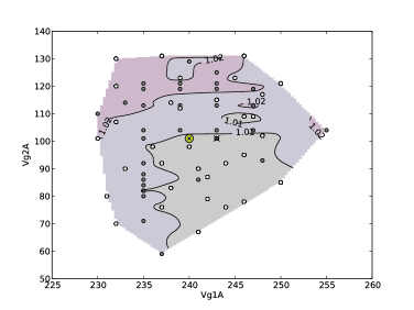
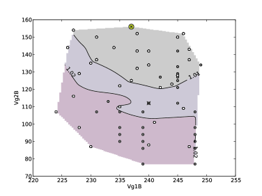
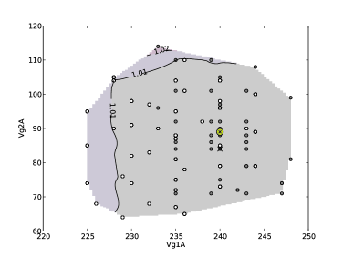
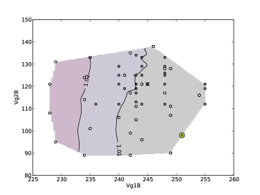
Figure 52: Hypermatrix tuning noise temperature maps as a function of $V_{\rm g1}$, on x-axis, and $V_{\rm g2}$, on y-axis. Colour scale ranges from red (highest noise temperatures) to light-grey (lowest noise temperatures), normalized to the lowest noise temperature.The best condensed noise temperature is enhanced by a yellow circule; system level test default by a black cross. Contours represents level of constant noise temperature. For each RCA, top panels: M1 (left), M2 (right); bottom panels: S1 (left), S2 (right). Note that the bias units are DEC units that are used to set the voltage in the DAE: see Table 4 for a rough conversion into physical units.

Appendix H Hypermatrix tuning: non linear plots

In Figures from  56 to 55 on each row two plots are showed for each detector (M-00, M-01, S-10, S-11) of the 30 GHz and 44 GHz Channels, each displaying the output voltage as a function of the extrapolated input antenna temperature: the panel on the right being a zoom of the one on the left. Data are corrected for the Back-End thermal drift; solid lines are obtained from the non linear gain model.
The pair of crosses in the zoomed plots represent the minimum and maximum of the estimated 4 K temperatures. This uncertainty is driven by the knowledge of the 4 K reference load temperature and to the BEU thermal drift.

LFI-24M

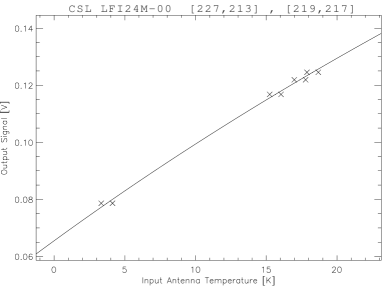
LFI-24S

Figure 53: Non linear response plots for 44 GHz LFI-24 channel.

LFI-25M

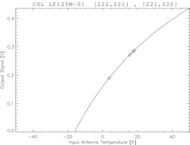
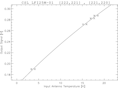
LFI-25S

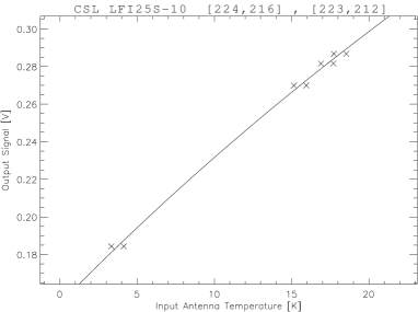
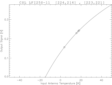
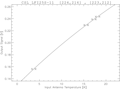
Figure 54: Non linear response plots for 44 GHz LFI-25 channel.

LFI-26M

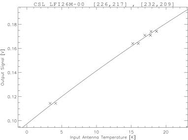
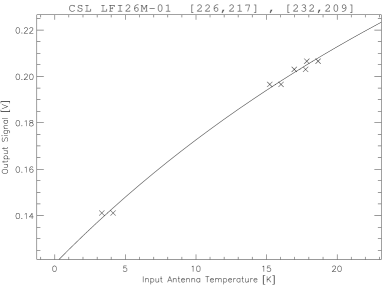
LFI-26S

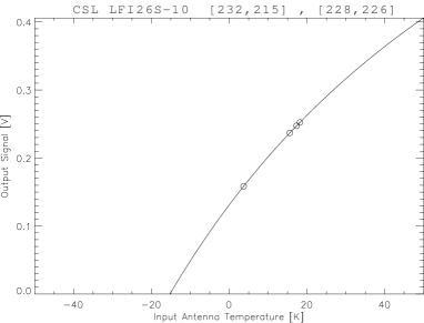
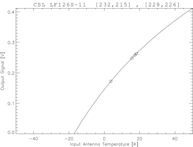
Figure 55: Non linear response plots for 44 GHz LFI-26 channel.

LFI-27M

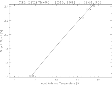
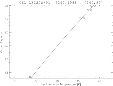
LFI-27S

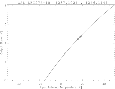
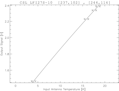
Figure 56: Non linear response plots for 30 GHz LFI-27 channel.

LFI-28M

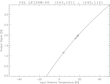
LFI-28S

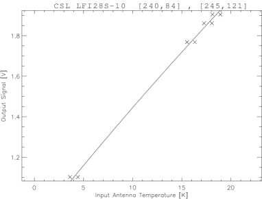
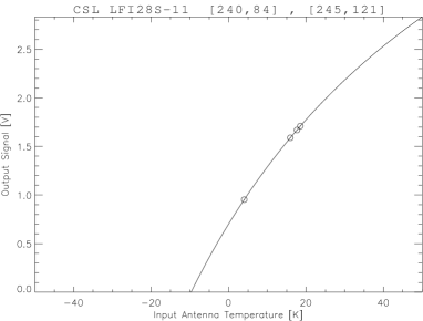
Figure 57: Non linear response plots for 30 GHz LFI-28 channel.

Appendix I Acronym list

Table 31: Acronym list.

Acronym
ACA	Amplifiers Chain Assembly
ADC	Analogue-to-Digital Converters
ADU	Analogue-to-Digital Units
ASD	Amplitude Spectral Density
BEM	Back-End Module
BEU	Back-End Unit
CMB	Cosmic Microwave Background
CPV	Calibration and Performance Verification
CSL	Centre Spatiale de Liége
DAE	Data Acquisition Electronics
DTCP	Daily Tele-Communication Period
FEM	Front-End Module
FPU	Focal Plane Unit
HFI	High Frequency Instrument
LFI	Low Frequency Instrument
LNA	Low Noise Amplifier
OMT	Ortho-Mode Transducer
PID	Proportional Integral Derivative
PSD	Power Spectral Density
RAA	Radiometer Array Assembly
RCA	Radiometer Chain Assembly
REBA	Radiometer Electronics Box Assembly
TSA	Temperature Stabilisation Assembly

References

- [1] J. A. Tauber, N. Mandolesi, J.-L. Puget et al. Planck pre-launch status: The Planck mission. A&A, 520:A1, 2010.
- [2] N. Mandolesi, M. Bersanelli, R. C. Butler et al. Planck pre-launch status: The Planck-LFI programme. A&A, 520:A3, 2010.
- [3] J. M. Lamarre, J. L. Puget and al.. Planck pre-launch status: The HFI instrument, from specification to actual performance. A&A, 520:A9, 2010.
- [4] J. A. Tauber, H. U. Norgaard-Nielsen, P. A. R. Ade et al. Planck pre-launch status: The optical system. A&A, 520:A2, 2010.
- [5] F. Villa, M. Bersanelli, C. Burigana et al. The Planck Telescope. In Experimental Cosmology at Millimetre Wavelengths, 616:224–228, 2002.
- [6] X. Dupac and J. Tauber. Scanning strategy for mapping the Cosmic Microwave Background anisotropies with Planck. A&A, 430:363–371, 2005.
- [7] M. Maris, M. Bersanelli, C. Burigana et al. The Flexible Planck Scanning Strategy. Memorie della Società Astronomica Italiana Supplement, 9:460, 2006.
- [8] A. Mennella, M. Bersanelli, R. C. Butler et al. Planck early results. III. First assessment of the Low Frequency Instrument in-flight performance. A&A, 536:A3, 2011.
- [9] Planck HFI Core Team. Planck early results. IV. First assessment of the High Frequency Instrument in-flight performance. A&A, 536:A4, 2011.
- [10] M. Bersanelli, N. Mandolesi, R. C. Butler et al. Planck pre-launch status: Design and description of the Low Frequency Instrument. A&A, 520:A4, 2010.
- [11] O. D’Arcangelo, L. Figini, A. Simonetto et al. The Planck-LFI flight model composite waveguides. Journal of Instrumentation, 4:2007, 2009.
- [12] L. Valenziano, F. Cuttaia, A. De Rosa et al. Planck-LFI: design and performance of the 4 Kelvin Reference Load Unit. Journal of Instrumentation, 4:2006, 2009.
- [13] J. M. Herreros, M. F. Gómez, R. Rebolo et al. The Planck-LFI Radiometer Electronics Box Assembly. Journal of Instrumentation, 4:2008, 2009.
- [14] M. Maris, M. Tomasi, S. Galeotta et al. Optimization of Planck-LFI on-board data handling. Journal of Instrumentation, 4:2018, 2009.
- [15] M. Seiffert, A. Mennella, C. Burigana et al. 1/f noise and other systematic effects in the Planck-LFI radiometers. A&A, 391:1185–1197, 2002.
- [16] A. Mennella, M. Bersanelli, M. Seiffert et al. Offset balancing in pseudo-correlation radiometers for CMB measurements. A&A, 410:1089–1100, 2003.
- [17] A. Zacchei, D. Maino, C. Baccigalupi et al. Planck early results. V. The Low Frequency Instrument data processing. A&A, 536:A5, 2011.
- [18] R. J. Davis, A. Wilkinson, R. D. Davies et al. Design, development and verification of the 30 and 44 GHz front-end modules for the Planck Low Frequency Instrument. Journal of Instrumentation, 4:2002, 2009.
- [19] E. Artal, B. Aja, M. L. de la Fuente et al. LFI 30 and 44 GHz receivers Back-End Modules. Journal of Instrumentation, 4:2003, 2009.
- [20] J. Varis, N. J. Hughes, M. Laaninen et al. Design, development, and verification of the Planck Low Frequency Instrument 70 GHz Front-End and Back-End Modules. Journal of Instrumentation, 4:2001, 2009.
- [21] F. Villa, L. Terenzi, M. Sandri et al. Planck pre-launch status: Calibration of the Low Frequency Instrument flight model radiometers. A&A, 520:A6, 2010.
- [22] A. Mennella, M. Bersanelli, R. C. Butler et al. Planck pre-launch status: Low Frequency Instrument calibration and expected scientific performance. A&A, 520:A5, 2010.
- [23] Planck Collaboration. Planck early results. II. The thermal performance of Planck. A&A, 536:A2, 2011.
- [24] Planck Collaboration. Planck early results. I. The Planck mission. A&A, 536:A1, 2011.
- [25] P. Meinhold, R. Leonardi, B. Aja et al. Noise properties of the Planck-LFI receivers. Journal of Instrumentation, 4:2009, 2009.
- [26] F. Cuttaia, A. Mennella, L. Stringhetti et al. Planck-LFI radiometers tuning. Journal of Instrumentation, 4:2013, 2009.
- [27] A. Mennella, F. Villa, L. Terenzi et al. The linearity response of the Planck-LFI flight model receivers. Journal of Instrumentation, 4:2011, 2009.
- [28] T. Poutanen, D. Maino, H. Kurki-Suonio, E. Keihänen and E. Hivon. Cosmic microwave background power spectrum estimation with the destriping technique. MNRAS, 353:43-58, 2004.
- [29] M. Tomasi, A. Mennella, S. Galeotta et al. Off-line radiometric analysis of Planck-LFI data. Journal of Instrumentation, 4:2020, 2009.
- [30] L. Terenzi, M. J. Salmon, A. Colin et al. Thermal susceptibility of the Planck-LFI receivers. Journal of Instrumentation, 4:2012-+, 2009.